Statistics 100A Homework 3 Solutions - UCLA Statistics
Statistics 100A Homework 3 Solutions - UCLA Statistics
Statistics 100A Homework 3 Solutions - UCLA Statistics

Create successful ePaper yourself
Turn your PDF publications into a flip-book with our unique Google optimized e-Paper software.
Chapter 4<br />
<strong>Statistics</strong> <strong>100A</strong><br />
<strong>Homework</strong> 3 <strong>Solutions</strong><br />
Ryan Rosario<br />
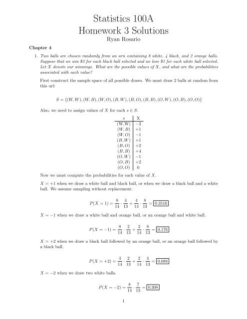
1. Two balls are chosen randomly from an urn containing 8 white, 4 black, and 2 orange balls.<br />
Suppose that we win $2 for each black ball selected and we lose $1 for each white ball selected.<br />
Let X denote our winnings. What are the possible values of X, and what are the probabilities<br />
associated with each value?<br />
First construct the sample space of all possible draws. We must draw 2 balls at random from<br />
this url:<br />
S = {(W, W ), (W, B), (W, O), (B, W ), (B, O), (B, B), (O, W ), (O, B), (O, O)}<br />
Also, we need to assign values of X for each s ∈ S.<br />
s X<br />
(W,W) −2<br />
(W, B) +1<br />
(W, O) −1<br />
(B, W ) +1<br />
(B, O) +2<br />
(B, B) +4<br />
(O, W ) −1<br />
(O, B) +2<br />
(O, O) 0<br />
Now we must compute the probabilities for each value of X.<br />
X = +1 when we draw a white ball and black ball, or when we draw a black ball and a white<br />
ball. We assume sampling without replacement:<br />
P (X = 1) = 8 4 4 8<br />
· + · = 0.3516<br />
14 13 14 13<br />
X = −1 when we draw a white ball and orange ball, or an orange ball and white ball.<br />
P (X = −1) = 8 2 2 8<br />
· + · = 0.176<br />
14 13 14 13<br />
X = +2 when we draw a black ball followed by an orange ball, or an orange ball followed by<br />
a black ball.<br />
X = −2 when we draw two white balls.<br />
P (X = +2) = 4 2 2 4<br />
· + · = 0.088<br />
14 13 14 13<br />
P (X = −2) = 8 7<br />
· = 0.308<br />
14 13<br />
1
X = +4 when two black balls are drawn.<br />
X = 0 when two orange balls are drawn.<br />
Then the probability distribution is given by<br />
P (X = +4) = 4 3<br />
· = 0.066<br />
14 13<br />
P (X = 0) = 2 1<br />
· = 0.011<br />
14 13<br />
x P(X = x)<br />
−2 0.308<br />
−1 0.176<br />
0 0.011<br />
+1 0.3516<br />
+2 0.088<br />
+4 0.066<br />
4. Five men a 5 women are ranked according to their scores on an examination. Assume that no<br />
two scores are alike and all 10! possible rankings are equally likely. Let X denote the highest<br />
ranking achieved by a woman. Find P (X = i), i = 1, 2, 3, . . . , 8, 9, 10..<br />
First off, note that the lowest possible position is 6, which means that all five women score<br />
worse than the five men. So P (X = i) = 0 for i = 7, 8, 9, 10 .<br />
Now let’s find how many different ways there are to arrange the 10 people such that the<br />
women all scored lower than the men. There are 5! ways to arrange the women and 5! ways<br />
to arrange the men, so<br />
P (X = 6) = 5!5!<br />
10!<br />
= 0.004<br />
Now consider the top woman scoring 5th on the exam.<br />
W<br />
There are 5 possible positions for the lower scoring women, � and � we have 4 women that must<br />
5<br />
be assigned to these ranks, which can be accomplished in different ways. Additionally,<br />
4<br />
these 5 women can be arranged in 5! ways, and the men can be arranged in 5! ways. Thus,<br />
P (X = 5) =<br />
� 5<br />
4<br />
�<br />
5!5!<br />
10!<br />
= 0.0198<br />
Similarly for P (X = 4), there are 6 positions for the 4 remaining women. The women can be<br />
arranged in 5! ways and the men can be arranged in 5! ways.<br />
P (X = 4) =<br />
� 6<br />
4<br />
2<br />
�<br />
5!5!<br />
10!<br />
= 0.0595
and so on...<br />
P (X = 3) =<br />
P (X = 2) =<br />
P (X = 1) =<br />
� 7<br />
4<br />
� 8<br />
4<br />
�<br />
5!5!<br />
10!<br />
�<br />
5!5!<br />
10!<br />
� 9<br />
4<br />
�<br />
5!5!<br />
10!<br />
≈ 0.139<br />
≈ 0.278<br />
= 0.5<br />
8. If the die in problem 7 is assumed fair, calculate the probabilities associated with the random<br />
variables in parts (a) through (d).<br />
Let X = f(X1, X2) where X1 and X2 are the faces showing on the first and second roll and<br />
f is given by<br />
(a) f(X1, X2) = max {X1, X2}<br />
The maximum value of the two rolls is 1 and the maximum value of the two rolls is 6.<br />
Therefore X = {1, 2, 3, 4, 5, 6}.<br />
x<br />
1<br />
2<br />
3<br />
4<br />
5<br />
Possibilities<br />
� �<br />
¥ and ¥<br />
� � �� �� � �<br />
¦ and ¥¦ or ¥ and ¦<br />
� � �� �� � �<br />
§ and ¥¦ or ¥¦ and §<br />
� � �� �� � �<br />
¨ and ¥¦§¨ or ¥¦§ and ¨<br />
� �<br />
�� �� � �<br />
© and ¥¦§¨© or ¥¦§¨ and ©<br />
� �<br />
�� �� � �<br />
P (X = x)<br />
1<br />
36<br />
3<br />
36<br />
5<br />
36<br />
7<br />
36<br />
9<br />
36<br />
6 � and ¥¦§¨©� or ¥¦§¨© and �<br />
(d) f(X1, X2) = X1 − X2<br />
In the extreme case, the first roll shows a 1 and the second shows a 6, or vice verse.<br />
Then, X = {−5, −4, −3, −2, −1, 0, 1, 2, 3, 4, 5}.<br />
x<br />
−5<br />
−4<br />
−3<br />
−2<br />
−1<br />
Possibilities<br />
�� ��<br />
¥, �<br />
�� � � ��<br />
¥, © , ¦, �<br />
�� � � � � ��<br />
¥, ¨ , ¦, © , §, �<br />
�� � � � � � � ��<br />
¥, § , ¦, ¨ , §, © , ¨, �<br />
�� � � � � � � � � ��<br />
¥, ¦ , ¦, § , §, ¨ , ¨, © , ©, �<br />
�� � � � � � � � � � � ��<br />
P (X = x)<br />
1<br />
36<br />
2<br />
36<br />
3<br />
36<br />
4<br />
36<br />
5<br />
36<br />
0 ¥, ¥ , ¦, ¦ , §, § , ¨, ¨ , ©, © , �, �<br />
For brevity, note that P (X = i) = P (X = −i) for i = 1, 2, 3, 4, 5, 6.<br />
3<br />
11<br />
36<br />
6<br />
36
14. Five distinct numbers are randomly distributed to players numbered 1 through 5. Whenever<br />
two players compare their numbers, the one with the highest one is declared the winner.<br />
Initially, players 1 and 2 compare their numbers; the winner then compares with player 3, and<br />
so on. Let X denote the number of times player 1 is a winner. Find P (X = i), i = 0, 1, 2, 3, 5.<br />
Find the probability that player 1 wins an even number of times.<br />
This problem ended up being much easier than the solution lead me to believe!<br />
We let X be the number of times player 1 is a winner.<br />
Let’s start with the case that player 1 never wins. That is, player 1 loses to player 2. If we<br />
construct the sample space, we would see that P (X = 0) = 1<br />
2 because exactly one-half of the<br />
5! permutations have the first number (player 1) greater than the second number (player 2).<br />
P (X = 0) =<br />
1<br />
25! 1 =<br />
5! 2<br />
Player 1 wins exactly 1 game if player 3 has a larger number than player 1, but player 1 has a<br />
larger number than player 2. The number of ways this can happen is the same as the number<br />
of ways that player 2 loses to player 1 and player 3 (hypothetically), etc. Per the solution I<br />
used, P (X = 1) = P (Y2 < Y1 < Y3) where Yi denotes the number given to player i. When<br />
i �= j �=, there are 3! ways to arrange the inequality Yi < Yj < Yk. Exactly one of these<br />
arrangements gives us the inequality Y2 < Y1 < Y3. Therefore,<br />
P (X = 1) =<br />
1<br />
3! 5! 1 1 = =<br />
5! 3! 6<br />
Now consider the case that player 1 wins exactly 2 games. This means Y1 > Y2 and Y1 > Y3<br />
but Y1 < Y4. The easiest way to do this is to consider all of the possible ways that this can<br />
happen,<br />
Then,<br />
S Player 1 wins 2 games. = {(Y1, Y2, Y3, Y4)}<br />
= {(3, 1, 2, 4), (3, 1, 2, 5), (3, 2, 1, 4), (3, 2, 1, 5), (4, 1, 2, 5), (4, 2, 1, 5)<br />
(4, 1, 3, 5), (4, 3, 1, 5), (4, 2, 3, 5), (4, 3, 2, 5)}<br />
P (X = 2) = 10<br />
5!<br />
= 1<br />
12<br />
To win 3 games, Y1 > Y2, and Y1 > Y3 and Y1 > Y4 but Y1 < Y5. One way to think of this is<br />
that we must restrict Y1 = 4 and Y5 = 5 and vary the others, giving 3! arrangements. Or, we<br />
can just list out the different combinations.<br />
S Player 1 wins 3 games. = {(Y1, Y2, Y3, Y4, Y5)}<br />
= {(4, 1, 2, 3, 5), (4, 2, 3, 1, 5), (4, 3, 2, 1, 5),<br />
(4, 1, 3, 2, 5), (4, 2, 1, 3, 5), (4, 3, 1, 2, 5)}<br />
P (X = 3) = 3! 1<br />
=<br />
5! 20<br />
4
To win all 4 games, Y1 > Y2 > Y3 > Y4 > Y5.<br />
S Player 1 wins 4 games. = {(Y1, Y2, Y3, Y4, Y5)}<br />
= {(5, ∗, ∗, ∗, ∗)}<br />
where ∗ denotes a wildcard meaning these players have some other number besides 5 here.<br />
For brevity, I do not list all of the arrangements, since we have enough information to solve<br />
the problem once we restrict Y1 = 5. Thus,<br />
Finally,<br />
P (X = 4) = 4! 1<br />
=<br />
5! 5<br />
P (X = even) = P (X = 2) + P (X = 4) = 1 1 17<br />
+ =<br />
12 5 60<br />
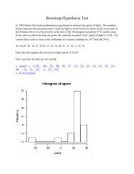
19. If the distribution of X is given by<br />
⎧<br />
0 b < 0<br />
1<br />
⎪⎨ 2 0 ≤ b < 1<br />
3<br />
F (b) = 5 1 ≤ b < 2<br />
4 2 ≤ b < 3<br />
calculate the probability mass function of X.<br />
⎪⎩<br />
5<br />
9<br />
10 3 ≤ b < 3.5<br />
1 b ≥ 3.5<br />
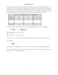
First we must find P (X = i), i = 0, 1, 2, 3, 3.5. To do that, we note that F (b) = P (X ≤ b)<br />
and that<br />
P (X = i) = P (X ≤ i) − P (X < i) = F (i) − P (X < i)<br />
This is really just a jump function between values of b. F is also called the cumulative<br />
distribution function (CDF).<br />
y 1<br />
0.9<br />
0.8<br />
0.7<br />
0.6<br />
0.5<br />
0.4<br />
0.3<br />
0.2<br />
0.1<br />
−2 −1<br />
0<br />
0 1 2 3 4 5<br />
x<br />
5
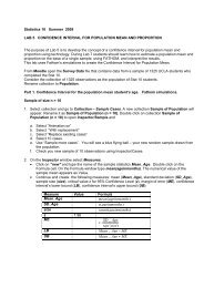
Which is represented as,<br />
P (X = i) F (i) − P (X < i) Calculation p(i)<br />
P (X = 0)<br />
P (X = 1)<br />
P (X = 2)<br />
P (X = 3)<br />
F (0) − P (X < 0)<br />
F (1) − P (X < 1)<br />
F (2) − P (X < 2)<br />
F (3) − P (X < 3)<br />
1<br />
2 − 0<br />
3 1<br />
5 − 2<br />
4 3<br />
5 − 5<br />
9 4 −<br />
1<br />
2<br />
1<br />
10<br />
1<br />
5<br />
1<br />
10 5<br />
P (X = 3.5) F (3.5) − P (X < 3.5) 1 − 9<br />
10<br />
y<br />
0.5<br />
0.4<br />
0.3<br />
0.2<br />
0.1<br />
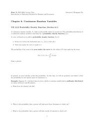
⎧ 1<br />
2 if x = 0<br />
1<br />
⎪⎨ 10 if x = 1<br />
1<br />
p(x) = 5 if x = 2<br />
⎪⎩<br />
1<br />
10 if x = 3<br />
1<br />
10 if x = 3.5<br />
0 otherwise<br />
0<br />
0 1 2 3<br />
x<br />
6<br />
10<br />
1<br />
10
20. A gambling book recommends the following “winning strategy” for the game of roulette. It<br />
recommends that a gambler bet $1 on red. If red appears (which has a probability of 18<br />
38 ),<br />
then the gambler should take her $1 profit and quit, If the gambler loses the bet (which has<br />
probability 20<br />
38 of occurring), she should make additional $1 bets on red on each of the next<br />
two spins of the roulette wheel and then quit. Let X denote the gambler’s winnings when she<br />
quits.<br />
(a) Find P (X > 0).<br />
First construct the sample space. Let R be the event that the ball lands on a red space<br />
and let R ′ be the complement of R. The sequence of spins will be of length 1 (if she<br />
wins on the first spin), or of length 3 (if she does not win on the first spin).<br />
S = � R, R ′ RR, R ′ R ′ R, R ′ RR ′ , R ′ R ′ R ′�<br />
If the wheel lands on a red space, then she wins $1 profit, otherwise she wins nothing<br />
and loses the $1 she bet. We can compute the values for X.<br />
s X<br />
R 1<br />
R ′ RR 1<br />
R ′ R ′ R −1<br />
R ′ RR ′ −1<br />
R ′ R ′ R ′ −3<br />
Then P (X > 0) = P (X = 1) which only happens one of two ways; she either wins on<br />
the first bet, or she loses on the first bet but wins on the next two spins. We assume<br />
that each spin of the roulette wheel is independent. Then,<br />
P (X > 0) = P (X = 1)<br />
= P (R) + P (R ′ RR)<br />
= 18 20 18 18<br />
+<br />
38 38 38 38<br />
= 0.5918<br />
The probability that she wins any profit is 0.5918.<br />
(b) Are you convinced that the strategy is indeed a “winning” strategy? Explain your answer!<br />
Typically this question would be answered after calculating E(X). Based on the probability<br />
in the previous part, it may seem like a winning strategy since the probability of<br />
profiting from the game is 0.5918 which is slightly better than flipping a coin. Actually,<br />
this is not a winning strategy, as we will see in the next part.<br />
7
(c) Find E(X).<br />
By definition,<br />
.<br />
E(X) =<br />
n�<br />
xP (X = x)<br />
i=1<br />
So, we need to construct the probability distribution.<br />
Then,<br />
x = P (X = x)<br />
� 3 = 0.1458<br />
−3 P (R ′ R ′ R ′ ) = � 20<br />
38<br />
−1 P (R ′ R ′ R) + P (R ′ RR ′ ) = 2 · 18<br />
38 · � 20<br />
38<br />
+1 (part a) = 0.5918<br />
� 2 = 0.2624<br />
E(X) = −3 · 0.1458 + (−1) · 0.2624 + 1 · 0.5918 = −0.108 ≈ −$0.11<br />
She should expect to lose 11 cents. Therefore, this is not a winning strategy.<br />
21. A total of 4 buses carrying 148 students from the same school arrives at a football stadium.<br />
The buses carry, respectively, 40, 33, 25, and 50 students. One of the students is randomly<br />
selected. Let X denote the number of students that were on the bus carrying this randomly<br />
selected student. One of the 4 bus drivers is also randomly selected selected. Let Y denote<br />
the number of students on her bus.<br />
(a) Which of E(X) or E(Y ) do you think is larger? Why?<br />
In the first sampling method, we draw one of 148 students at random. Naturally, the<br />
probability of choosing a student from the fullest bus is higher than the probability of<br />
drawing a student from the other buses. Thus, the fuller buses are weighted higher than<br />
the other buses, so we would expect E(X) to be larger. In the second method, one of the<br />
four bus drivers is randomly selected. Each bus driver is equally likely to be chosen!<br />
Each bus is weighted the sum, therefore, E(Y ) ≤ E(X). Equality holds when each bus<br />
contains the same number of students.<br />
Analogy: Consider calculating your GPA two different ways. Suppose your grades<br />
this quarter are as follows: A, C, C. The class that you earned an A in is worth 5 units<br />
and the classes you earned the Cs in are worth 4 units. Computing your GPA using the<br />
standard method of weighting the grades by units would weight the higher grade heavier<br />
than each of the two Cs. This calculation is similar to the calculation of E(X). The<br />
GPA in this case is 3.00.<br />
Now suppose we ignore the course units and recompute the GPA such that each grade<br />
is weighted the same. Then the GPA is 2.67. This calculation is similar to E(Y ). In<br />
this particular case, we see that the weighted method is higher.<br />
8
(b) Compute E(X) and E(Y ).<br />
First we need the probability distributions for X and Y .<br />
X corresponds to the method of drawing a student at random. The probability that a<br />
student comes from bus i, i = {A, B, C, D} is simply the number of students on that bus<br />
divided by the total number of students.<br />
x = P (X = x)<br />
40<br />
33<br />
25<br />
50<br />
40<br />
148<br />
33<br />
148<br />
25<br />
148<br />
50<br />
148<br />
Then, E(X) = 40 · 40 33 25 50<br />
148 + 33 · 148 + 25 · 148 + 50 · 148 = 39.28 .<br />
Y corresponds to the method of drawing a bus driver at random. The probability that<br />
a bus driver comes from a particular bus is constant, 1<br />
4 .<br />
x = P (X = x)<br />
40<br />
33<br />
25<br />
50<br />
1<br />
4<br />
1<br />
4<br />
1<br />
4<br />
Then, E(Y ) = 40 · 1 1 1 1<br />
4 + 33 · 4 + 25 · 4 + 50 · 4 = 37 .<br />
30. A person tosses a fair coin until a tail appears for the first time. If the tail appears on the nth<br />
flip, the person wins 2 n dollars. Let X denote the player’s winnings. This problem is known<br />
as the St. Petersburg paradox.<br />
This is an example of the geometric distribution. We use the geometric distribution when we<br />
want to calculate the probability that it takes n trials to get a success. In this case, a success<br />
is the event that a tail is showing.<br />
(a) Show that E(X) = +∞.<br />
1<br />
4<br />
Proof. We know that X denotes the player’s winnings, so X = 2n �<br />
for n ≥ 1. The<br />
n.<br />
Then,<br />
probability that a player wins on the nth game is � 1<br />
2<br />
E(X) =<br />
∞�<br />
xP (X = x) =<br />
i=1<br />
9<br />
∞�<br />
2 n ·<br />
i=1<br />
� �n 1<br />
=<br />
2<br />
∞�<br />
1 = +∞<br />
i=1
(b) Would you be willing to play $1 million to play this game once?<br />
Hell no ! Suppose you pay $1 million to play once and you win on the first game. You<br />
only win $2. Suppose you lose on the first game (which is likely), then you lost your bet.<br />
E(X) = ∞ is the expected value in the long run, not on one game!<br />
(c) Would you be willing to play $1 million for each game if you could play for as long as<br />
you liked and only had to settle up when you stopped playing?<br />
Yes , the expectation in the long run is “something large,” so we could expect to profit.<br />
This is not a universally accepted answer though. From Wikipedia,<br />
“According to the usual treatment of deciding when it is advantageous and therefore<br />
rational to play, you should therefore play the game at any price if offered the opportunity.<br />
Yet, in published descriptions of the paradox, e.g. (Martin, 2004), many people<br />
expressed disbelief in the result. Martin quotes Ian Hacking as saying ”few of us would<br />
pay even $25 to enter such a game” and says most commentators would agree.”<br />
I highly recommend the Wikipedia article on the St. Petersburg paradox!<br />
37. Find Var (X) and Var (Y ) for X and Y as given in Problem 21.<br />
By definition,<br />
Thus,<br />
E(X 2 ) =<br />
Similarly,<br />
n�<br />
i=1<br />
�<br />
Var (X) = E (X − E(X)) 2�<br />
= E(X 2 ) − E(X) 2<br />
x x 2 P (X = x)<br />
40 1600 40<br />
148<br />
33 1089 33<br />
148<br />
25 625 25<br />
148<br />
50 2500 50<br />
148<br />
x 2 P (X = x) = 1600 · 40 33 25 50<br />
+ 1089 · + 625 · + 2500 · = 1625.4<br />
148 148 148 148<br />
Var (X) = E(X 2 ) − E(X) 2 = 1625.4 − 39.28 2 = 82.2<br />
y y 2 P (Y = y)<br />
40 1600 1<br />
4<br />
33 1089 1<br />
4<br />
25 625 1<br />
4<br />
50 2500 1<br />
4<br />
E(Y ) = 1<br />
(1600 + 1089 + 625 + 2500) = 1453.5<br />
4<br />
Var (Y ) = E(Y 2 ) − E(Y ) 2 = 1453.5 − 37 2 = 84.5<br />
10
38. If E(X) = 1 and Var (X) = 5, find<br />
Recall the following properties of expectation and variance<br />
E(c) = c, E(cX) = cE(X), E(X + Y ) = E(X) + E(Y )<br />
Var (c) = 0, Var (cX) = c 2 Var (x) , Var (X + Y ) = Var (X)+Var (Y ) iff X, Y indpdt<br />
�<br />
(a) E (2 + X) 2�<br />
�<br />
E (2 + X) 2�<br />
(b) Var (4 + 3X)<br />
Var (x) = E(X 2 ) − E(X) 2<br />
= E [(2 + X) (2 + X)]<br />
= E � 4 + X 2 + 4X �<br />
= E(4) + E(X 2 ) + E(4X)<br />
= 4 + E(X 2 ) + 4E(X)<br />
Recall that Var (x) = E(X 2 ) − E(X) 2<br />
= 4 + � Var (X) + E(X) 2� + 4E(X)<br />
= 4 + � 5 + 1 2� + 4 · 1<br />
= 14<br />
Var (4 + 3X) = Var (4) + Var (3X)<br />
= 0 + 3 2 Var (X)<br />
= 9 · Var (X)<br />
= 9 · 5<br />
= 45<br />
11