3. Continuous Random Variables

3. Continuous Random Variables
Statistics and probability: 3-1
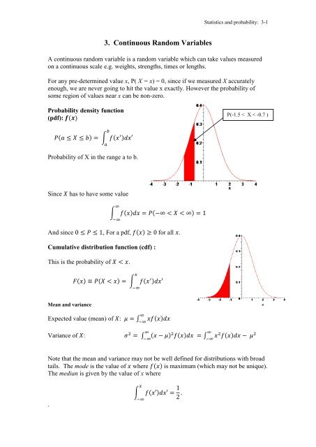
A continuous random variable is a random variable which can take values measured
on a continuous scale e.g. weights, strengths, times or lengths.
For any pre-determined value x, P( X = x) = 0, since if we measured X accurately
enough, we are never going to hit the value x exactly. However the probability of
some region of values near x can be non-zero.
Probability density function
(pdf):
∫
Probability of X in the range a to b.
Since has to have some value
∫
And since , For a pdf, for all .
Cumulative distribution function (cdf) :
This is the probability of .
Mean and variance
∫
Expected value (mean) of : ∫
Variance of : ∫
Note that the mean and variance may not be well defined for distributions with broad
tails. The mode is the value of where is maximum (which may not be unique).
The median is given by the value of x where
.
∫
∫
P(-1.5 < X < -0.7 )

Uniform distribution
The continuous random variable has the
Uniform distribution between and , with
if
{
, for short.
Statistics and probability: 3-2
Roughly speaking, , if X can only take values between and , and
any value of within these values is as likely as any other value.
Mean and variance: for ,
Proof:
Let y be the distance from the mid-point, , and the width be
. Then since means add
〈 〉
〈 〉
Unsurprisingly the mean is the midpoint.
∫
Occurrence of the Uniform distribution
∫
1) Waiting times from random arrival time until a regular event (see below)
2) Engineering tolerances: e.g. if a diameter is quoted "�0.1mm", it sometimes
assumed (probably incorrectly) that the error has a U(-0.1, 0.1) distribution.
3) Simulation: programming languages often have a standard routine for simulating
the U(0, 1) distribution. This can be used to simulate other probability distributions.
f(x)
and
∫
*
+
� �
1 2
(
)
x

Example: Disk wait times
Statistics and probability: 3-3
In a hard disk drive, the disk rotates at 7200rpm. The wait time is defined
as the time between the read/write head moving into position and the
beginning of the required information appearing under the head.
(a) Find the distribution of the wait time.
(b) Find the mean and standard deviation of the wait time.
(c) Booting a computer requires that 2000 pieces of information are read from random
positions. What is the total expected contribution of the wait time to the boot time,
and rms deviation?
Solution
Rotation time = 8.33ms. Wait time can be anything between 0 and 8.33ms and each
time in this range is as likely as any other time. Therefore, distribution of the wait
time is U(0, 8.33ms) (i. . � 1 = 0 and � 2 = 8.33ms).
For 2000 reads the mean time is 2000 4.2 ms = 8.3s.
The variance is 2000 5.7ms 2 = 0.012s 2 , so � =0.11s.
Exponential distribution
The continuous random variable has the
Exponential distribution, parameter if:
{
;
Relation to Poisson distribution: If a Poisson process has constant rate , the mean
after a time is . The probability of no-occurrences in this time is

Statistics and probability: 3-4
If is the pdf for the first occurrence, then the probability of no occurrences is also
given by
So equating the two ways of calculating the probability we have
Now we can differentiate with respect to giving
hence :.the time until the first occurrence (and between subsequent
occurrences) has the Exponential distribution, parameter .
Occurrence
1) Time until the failure of a part.
2) Times between randomly happening events
Mean and variance
∫
∫
Example: Reliability
∫
∫
[ ] ∫
∫
∫
[ ] ∫
The time till failure of an electronic component has an Exponential distribution and it
is known that 10% of components have failed by 1000 hours.
(a) What is the probability that a component is still working after 5000 hours?
(b) Find the mean and standard deviation of the time till failure.
Solution
(a) Let Y = time till failure in hours;
∫
[
]

∫
∫
(b) Mean = = 9491 hours.
Standard deviation =√ = √
Normal distribution
[ ]
[ ]
= 9491 hours.
Statistics and probability: 3-5
The continuous random variable has the Normal distribution if the pdf is:
√
The parameter � is the mean and and the
variance is � 2 . The distribution is also
sometimes called a Gaussian distribution.
The pdf is symmetric about �. X lies between �
- 1.96� and � + 1.96� with probability 0.95 i.e.
X lies within 2 standard deviations of the mean
approximately 95% of the time.
Normalization
[non-examinable]
cannot be integrated analytically for general ranges, but the full range can be
integated as follows. Define
I �
�
�
��
dx e
2
2
�(
x��
)
�x
2 �
2
2�
2�
�
�
��
dx e
Then switching to polar co-ordinates we have

I
2
�
�
�
��
dx e
�
2
� 2�
���
e
��
Hence I =
2
� x
2�
2
2
�
r
�
2
2�
�
��
�
�
��
0
dy e
�
2�
2
� y
2
�
2
� 2��
�
�
��
�
�
��
dxdy e
2
2
x � y
�
2
2�
�
�
0
�
�
2�
0
rdrd�
e
2
2�� and the normal distribution integrates to one.
Statistics and probability: 3-6
2
r
�
2
2�
� 2�
�
0
�
rdre
Mean and variance
The mean is because the distribution is symmetric about (or you can check
explicitly by integrating by parts). The variance can be also be checked by integrating
by parts:
∫
√
[
∫
√ ]
Occurrence of the Normal distribution
√
1) Quite a few variables, e.g. human height, measurement errors, detector noise.
(Bell-shaped histogram).
2) Sample means and totals - see below, Central Limit Theorem.
3) Approximation to several other distributions - see below.
Change of variable
The probability for X in a range around is for a distribution is given by
The probability should be the same if it is written in terms of another
variable . Hence
∫
√
∫
√
∫
2
r
�
2
2�

Standard Normal distribution
Statistics and probability: 3-7
There is no simple formula for ∫ , so numerical integration (or tables) must
be used. The following result means that it is only necessary to have tables for one
value of and .
If , then
This follows when changing variables since
√
hence
Z is the standardised value of X; N(0, 1) is the standard Normal distribution. The
Normal tables give values of Q=P(Z � z), also called �(z), for z between 0 and 3.59.
Outside of exams this is probably best evaluated using a computer package (e.g.
Maple, Mathematica, Matlab, Excel); for historical reasons you still have to use
tables.
Example: Using standard Normal tables (on course web page and in exams)
If Z ~ N(0, 1):
(a)
(b) (by symmetry)
=
= 1 - 0.8413 = 0.1587
(c)
(d)
= 0.6915.
= �(1.5) - �(0.5)
= 0.9332 - 0.6915
= 0.2417.
∫
√

(e) - Using interpolation:
(f)
Using tables "in reverse", .
Statistics and probability: 3-8
( )
(g) Finding a range of values within which lies with probability 0.95:
The answer is not unique; but suppose we want an interval which is symmetric about
zero i.e. between -d and d.
Tail area = 0.025
� P(Z � d) = �(d) = 0.975
Using the tables "in reverse", d = 1.96.
� range is -1.96 to 1.96.
Example: Manufacturing variability
The outside diameter, X mm, of a copper pipe is N(15.00, 0.02 2 ) and the fittings for
joining the pipe have inside diameter Y mm, where Y ~ N(15.07, 0.022 2 ).
(i) Find the probability that X exceeds 14.99 mm.
(ii) Within what range will X lie with probability 0.95?
(iii) Find the probability that a randomly chosen pipe fits into a randomly chosen
fitting (i.e. X < Y).
Solution
(i)
(ii) From previous example
i.e. (
(
)
)
P=0.025
lies in (-1.96, 1.96) with probability 0.95.
P=0.025

i.e. the required range is 14.96mm to 15.04mm.
Statistics and probability: 3-9
(iii) For we want ). To answer this we need to know the
distribution of
Distribution of the sum of Normal variates
Remember than means and variances of independent random variables just add. So if
are independent and each have a normal distribution ,
we can easily calculate the mean and variance of the sum. A special property of the
Normal distribution is that the distribution of the sum of Normal variates is also a
Normal distribution. So if are constants then:
2 2 2 2 2 2
c X � c X �� �c
X ~ N( c � ���c � , c � � c � ��
c � )
1 1 2 2
n n
1 1 n n 1 1 2 2 n n
Proof that the distribution of the sum is Normal is beyond scope. Useful special cases
for two variables are
If all the X's have the same distribution i.e. � 1 = � 2 = ... = � n = � , say and � 1 2 = �2 2
= ... = � n 2 = � 2 , say, then:
(iii) All c i = 1: X 1 + X 2 + ... + X n ~ N(n�, n� 2 )
(iv) All c i = 1/n: X =
X1 � X 2 ��� X
n
n
~ N(�, � 2 /n)
The last result tells you that if you average n identical independent noisy
measurements, the error decreases by √ . (variance goes down as ).
Example: Manufacturing variability (iii)
Find the probability that a randomly chosen pipe fits into a randomly chosen
fitting (i.e. X < Y).
Using the above results
Hence
(
√ )

Example: detector noise
Statistics and probability: 3-10
A detector on a satellite can measure T+g, the temperature T of a source with a
random noise g, where g ~ N(0, 1K 2 ). How many detectors with independent noise
would you need to measure T to an rms error of 0.1K?
Answer: We can estimate the temperature from n detectors by calculating the mean
from each. The variance of the mean will be 1K 2 /n where n is the number of detectors.
An rms error of 0.1K corresponds to a variance of 0.01 K 2 , hence we need n=100
detectors.
Normal approximations
Central Limit Theorem: If X1 , X2 , ... are independent random variables with the
same distribution, which has mean � and variance (both finite), then the sum
n
�
i�1
X i
tends to the distribution as .
Hence: The sample mean X n = �
i�
for large n.
1
n
n 1
X i
is distributed approximately as N(�, � 2 /n)
For the approximation to be good, n has to be bigger than 30 or more for skewed
distributions, but can be quite small for simple symmetric distributions.
The approximation tends to have much better fractional accuracy near the peak than
in the tails: don’t rely on the approximation to estimate the probability of very rare
events.
Example: Average of n samples from a uniform distribution:

Normal approximation to the Binomial
Statistics and probability: 3-11
If X ~ B(n, p) and n is large and np is not too near 0 or 1, then X is approximately
N(np, np(1-p)).
The probability of getting from the Binomial distribution can be approximated as
the probability under a Normal distribution for getting in the range from to
. For example can be approximated as ∫
Normal distribution:
where is the
Example: I toss a coin 1000 times, what is the probability that I get more than 550
heads?
Answer: The number of heads has a binomial distribution with mean np=500 and
variance So the number of heads can be approximated as
. Hence
(
√

Quality control example:
Statistics and probability: 3-12
The manufacturing of computer chips produces 10% defective chips. 200 chips are
randomly selected from a large production batch. What is the probability that fewer
than 15 are defective?
Answer: the mean is , variance
. So if is the number of defective chips, approximately ,
hence
(
)
√
[ ]
This compares to the exact Binomial answer ∑
. The
Binomial answer is easy to calculate on a computer, but the Normal approximation is
much easier if you have to do it by hand. The Normal approximation is about right,
but not accurate.
Normal approximation to the Poisson
If Poisson
parameter and
is large (> 7, say),
then has
approximately a
distribution.

Example: Stock Control
Statistics and probability: 3-13
At a given hospital, patients with a particular virus arrive at an average rate of once
every five days. Pills to treat the virus (one per patient) have to be ordered every 100
days. You are currently out of pills; how many should you order if the probability of
running out is to be less than 0.005?
Solution
Assume the patients arrive independently, so this is a Poisson process, with rate 0.2 /
day.
Therefore, Y, number of pills needed in 100 days, ~ Poisson, = 100 x 0.2 = 20.
We want , or (
) under the Normal
approximation, where a probability of 0.995 corresponds (from tables) to 2.575.
Since this corresponds to.
√ , so we
need to order pills.
Comment
Let’s say the virus is deadly, so we want to make sure the probability is less than 1
in a million, 10 -6 . A normal approximation would give 4.7 above the mean, so
pills. But surely getting just a bit above twice the average number of cases
is not that unlikely??
Yes indeed, the assumption of independence is extremely unlikely to be valid.
Viruses tend to be infectious, so occurrences are definitely not independent. There
is likely to be a small but significant probability of a large number of people being
infected simultaneously – a much larger number of pills needs to be stocked to be
safe.
Don’t use approximations that are too simple if their failure might be
important! Rare events in particular are often a lot more likely than predicted by
(too-) simple approximations for the probability distribution.