3. Continuous Random Variables

Example: detector noise
Statistics and probability: 3-10
A detector on a satellite can measure T+g, the temperature T of a source with a
random noise g, where g ~ N(0, 1K 2 ). How many detectors with independent noise
would you need to measure T to an rms error of 0.1K?
Answer: We can estimate the temperature from n detectors by calculating the mean
from each. The variance of the mean will be 1K 2 /n where n is the number of detectors.
An rms error of 0.1K corresponds to a variance of 0.01 K 2 , hence we need n=100
detectors.
Normal approximations
Central Limit Theorem: If X1 , X2 , ... are independent random variables with the
same distribution, which has mean � and variance (both finite), then the sum
n
�
i�1
X i
tends to the distribution as .
Hence: The sample mean X n = �
i�
for large n.
1
n
n 1
X i
is distributed approximately as N(�, � 2 /n)
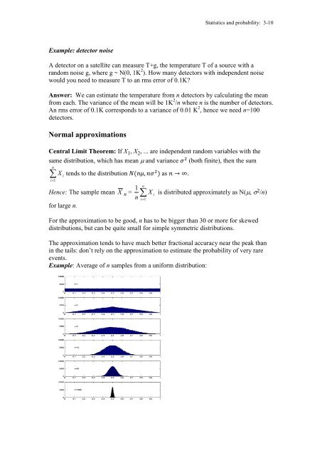
For the approximation to be good, n has to be bigger than 30 or more for skewed
distributions, but can be quite small for simple symmetric distributions.
The approximation tends to have much better fractional accuracy near the peak than
in the tails: don’t rely on the approximation to estimate the probability of very rare
events.
Example: Average of n samples from a uniform distribution: