Crystals, Liquid Crystals and Superfluid Helium on Curved Surfaces.

<strong>Crystals</strong>, <strong>Liquid</strong> <strong>Crystals</strong> <strong>and</strong> <strong>Superfluid</strong> <strong>Helium</strong> on Curved 

Surfaces. 

A dissertation presented 

by 

Vincenzo Vitelli 

to 

The Department of Physics 

in partial fulfillment of the requirements 

for the degree of 

Doctor of Philosophy 

in the subject of 

Physics 

Harvard University 

Cambridge, Massachusetts 

May 2006

c○2006 - Vincenzo Vitelli 

All rights reserved.

Thesis advisor Author 

David R. Nelson Vincenzo Vitelli 

<strong>Crystals</strong>, <strong>Liquid</strong> <strong>Crystals</strong> <strong>and</strong> <strong>Superfluid</strong> <strong>Helium</strong> on Curved Surfaces. 

Abstract 

In this thesis we study the ground state of ordered phases grown as thin layers on 

substrates with smooth spatially varying Gaussian curvature. The Gaussian curvature 

acts as a source for a one body potential of purely geometrical origin that controls the 

equilibrium distribution of the defects in liquid crystal layers, thin films of He 4 <strong>and</strong> 

two dimensional crystals on a frozen curved surface. For superfluids, all defects are 

repelled (attracted) by regions of positive (negative) Gaussian curvature. For liquid 

crystals, charges between 0 <strong>and</strong> 4π are attracted by regions of positive curvature while 

all other charges are repelled. As the thickness of the liquid crystal film increases, 

transitions between two <strong>and</strong> three dimensional defect structures are triggered in the 

ground state of the system. Thin spherical shells of nematic molecules with planar 

anchoring possess four short 1 disclination lines but, as the thickness increases, a three 

2 

dimensional escaped configuration composed of two pairs of half-hedgehogs becomes 

energetically favorable. Finally, we examine the static <strong>and</strong> dynamical properties that 

distinguish two dimensional crystals constrained to lie on a curved substrate from 

their flat space counterparts. A generic mechanism of dislocation unbinding in the 

presence of varying Gaussian curvature is presented. We explore how the geometric 

potential affects the energetics <strong>and</strong> dynamics of dislocations <strong>and</strong> point defects such 

as vacancies <strong>and</strong> interstitials. 

iii

Contents 

Title Page . . . . . . . . . . . . . . . . . . . . . . . . . . . . . . . . . . . . i 

Abstract . . . . . . . . . . . . . . . . . . . . . . . . . . . . . . . . . . . . . iii 

Table of Contents . . . . . . . . . . . . . . . . . . . . . . . . . . . . . . . . iv 

Acknowledgments . . . . . . . . . . . . . . . . . . . . . . . . . . . . . . . . vi 

Dedication . . . . . . . . . . . . . . . . . . . . . . . . . . . . . . . . . . . . viii 

1 Introduction 1 

1.1 Introduction . . . . . . . . . . . . . . . . . . . . . . . . . . . . . . . . 2 

1.1.1 Experimental motivation . . . . . . . . . . . . . . . . . . . . . 2 

1.1.2 Mechanisms of coupling between defects <strong>and</strong> curvature . . . . 5 

1.1.3 Cross-over between 2D <strong>and</strong> 3D physics . . . . . . . . . . . . . 13 

1.1.4 Outline of the thesis . . . . . . . . . . . . . . . . . . . . . . . 14 

2 Bond-orientational order on a corrugated substrate. 16 


2.2 Hexatic order on a surface . . . . . . . . . . . . . . . . . . . . . . . . 21 

2.2.1 Electrostatic analogy . . . . . . . . . . . . . . . . . . . . . . . 21 

2.2.2 Defect free texture . . . . . . . . . . . . . . . . . . . . . . . . 26 

2.2.3 Energetics of defect pairs on a Gaussian bump . . . . . . . . . 30 

2.3 Curvature induced defect generation . . . . . . . . . . . . . . . . . . 35 

2.3.1 Onset of the defect-dipole instability . . . . . . . . . . . . . . 35 

2.3.2 Numerical investigation of defect-unbinding transitions . . . . 39 

2.3.3 Single vortex instability . . . . . . . . . . . . . . . . . . . . . 44 

2.3.4 Lattice of bumps, valleys <strong>and</strong> saddle points . . . . . . . . . . . 48 

2.4 Defect Deconfinement . . . . . . . . . . . . . . . . . . . . . . . . . . 50 

2.5 Conclusion . . . . . . . . . . . . . . . . . . . . . . . . . . . . . . . . . 59 

3 <strong>Liquid</strong> crystal textures in thick spherical shells. 60 


3.2 Textures . . . . . . . . . . . . . . . . . . . . . . . . . . . . . . . . . . 64 

3.2.1 Tilted molecules on a sphere . . . . . . . . . . . . . . . . . . . 66 

3.2.2 Nematic Texture . . . . . . . . . . . . . . . . . . . . . . . . . 68 

3.3 Stability of liquid crystal textures to thermal fluctuations . . . . . . 80 

iv

Contents v 

3.4 Valence transitions in thick nematic shells . . . . . . . . . . . . . . . 88 

3.4.1 Slab geometry . . . . . . . . . . . . . . . . . . . . . . . . . . . 88 

3.4.2 Extrapolation to thin spherical shells . . . . . . . . . . . . . . 94 

3.5 Conclusion . . . . . . . . . . . . . . . . . . . . . . . . . . . . . . . . . 97 

4 <strong>Superfluid</strong> films on a curved surface. 99 

5 Defects <strong>and</strong> crystalline order on curved surfaces. 112 


5.2 Basic Formalism . . . . . . . . . . . . . . . . . . . . . . . . . . . . . 114 

5.3 Geometric Frustration . . . . . . . . . . . . . . . . . . . . . . . . . . 117 

5.4 Geometric potential for dislocations . . . . . . . . . . . . . . . . . . 119 

5.5 Dislocation unbinding <strong>and</strong> Grain Boundaries . . . . . . . . . . . . . 123 

5.6 Glide suppression . . . . . . . . . . . . . . . . . . . . . . . . . . . . . 125 

5.7 Vacancies, Interstitials <strong>and</strong> Impurities . . . . . . . . . . . . . . . . . 127 

A Green’s function <strong>and</strong> Isothermal Coordinates 131 

B Geometric Potential 137 

C Free energy on a corrugated plane 142 

D Bump with a boundary 150 

E Free energy of a vector field on a sphere 162 

F <strong>Liquid</strong> crystal textures <strong>and</strong> conformal mappings 170 

G Vibrational spectrum of colloidal molecules 179 

H Perturbation theory of curved crystals 188 

I Curvature induced finite size effects 193 

J Numerical Methods 199 

Bibliography 203

Acknowledgments 

This work originates from the inspiring mentorship of Professor D. R. Nelson 

to whom goes my lasting gratitude for patiently guiding my first steps in scientific 

research while always encouraging independence of thought. 

I had the privilege to have Professors B. I. Halperin <strong>and</strong> D. A. Weitz on 

my thesis committee <strong>and</strong> I wish to thank them for enlightening interactions. As a 

beginning graduate student, I attended some stimulating courses taught by Professors 

S. Sachdev <strong>and</strong> D. S. Fisher that greatly fostered my interest in condensed matter 

theory. One of the most rewarding aspects of my PhD experience at Harvard has been 

the unique chance to informally interact with a number of very talented graduate 

students <strong>and</strong> postdoctoral fellows from whom I learned a lot <strong>and</strong> shared moments of 

fun: M. Desai, A. Delmaestro, A. Imambekov, I. Finkler, W. P. Wong, R. Barnett, D. 

Podolsky, H. Chen, O. White, K. Papadodimas, E. Katifori, G. Rafael, A. Polkolnikov, 

R. da Silveira, Y. Kafri, J. Qiang, C. Kilic <strong>and</strong> P. J. Lu. A special thanks goes to A. 

Fern<strong>and</strong>ez-Nieves, A. M. Turner <strong>and</strong> J. B. Lucks with whom I collaborated on the 

work discussed in chapters I, IV <strong>and</strong> V respectively. 

I wish to thank the administrative staff of the Physics Department in par- 

ticular Dr. D. Norcross <strong>and</strong> S. Ferguson for providing constant help. 

As an undergraduate at Imperial College London, I have been fortunate 

to meet many inspiring lecturers that I wish to thank for their crucial help <strong>and</strong> 

generosity particularly Professors M. P. Blencowe, J. P. Connerade, P. L. Knight, A. 

McKinnon, M. B. Plenio <strong>and</strong> D. Vvedensky. An undergraduate bursary from the 

Nuffield foundation allowed me to try research first h<strong>and</strong> <strong>and</strong> to spend a stimulating 

vi

Acknowledgments vii 

semester as a visiting student working under the supervision of Dr. T. S. Chang at 

MIT. 

I wish to thank my family <strong>and</strong> A. Alyahya for their support throughout.

To don Rocco, to my gr<strong>and</strong>parents. 

viii

Chapter 1 

Introduction 

1

Chapter 1: Introduction 2 

1.1 Introduction 

The physics of 2D condensed matter systems is a rich <strong>and</strong> mature subject 

[1, 2]. In this thesis we study the effects induced in the ground state of a thin layer 

of material by the Gaussian curvature of the substrate on which it is deposited. Spe- 

cific examples include liquid crystalline order at the curved interface between two 

immiscible fluids, thin films of He 4 wetting a corrugated substrate <strong>and</strong> two dimen- 

sional crystals <strong>and</strong> liquid crystals on a lithographically prepared curved substrate. 

While these systems are physically distinct, some of the consequences of the varying 

Gaussian curvature of the substrate or interface can be understood within a unifying 

perspective. It is the purpose of this introduction to illustrate basic concepts <strong>and</strong> 

suggest possible experimental tests of the theoretical ideas presented in this thesis. 

1.1.1 Experimental motivation 

Recent experimental investigations of spherical crystallography have already 

revealed complex ground state structures riddled with topological defects forced in by 

the topology of the underlying curved space [3]. Fig. 1.1 shows a colloidosome engi- 

neered in the Weitz lab with 0.5 µm colloidal particles self assembled on an oil-water 

interface. Besides its intriguing technological applications as a microcapsule for drug 

delivery, the colloidosome provides a natural laboratory to explore (under controlled 

experimental conditions) basic scientific questions of curved space crystallography rel- 

evant to a larger class of materials including those of biological origin such as viruses 

<strong>and</strong> clathrin-coated pits [5, 6, 7, 8, 9]. Confocal microscopy of small colloidosomes


Figure 1.1: Image of a colloidosome by confocal microscopy (courtesy of the Weitz 

lab). The right panel shows the arrangement of 5 <strong>and</strong> 7-fold disclinations, represented 

as red <strong>and</strong> yellow dots respectively, in the ground state of a spherical crystal 

(reproduced from Ref.[4]). 

reveals 12 five-fold coordinated lattice sites symmetrically placed approximately at 

the vertices of an icosahedron inscribed in the sphere. When the droplet radius R 

is larger than 5-6 times the colloidal radius, the nucleation of grain boundary scars 

emanating from each disclination becomes energetically favorable [4, 10]. 

<strong>Liquid</strong> crystal (LC) analogs of these systems can be realized by trapping a 

thin layer of thermotropic liquid crystals in a double emulsion [11]. Fig. 1.2 shows 

four s = 1 

2 

disclination lines visible under crossed polarizers as double-brushes, which 

confer to the colloidal particle an effective valence Z = 4 [12, 13]. The disclinations in 

the droplet represented in Fig. 1.2 do not lie exactly at the vertices of a tetrahedron 

because of the non uniform thickness of the layer. An alternative route to colloids 

with a valence is provided by mono-layers of lyotropic nematogens [11]. The main 

technological thrust behind these experiments is the desire to functionalize droplets 

or colloids using chemical linkers. Such a tetravalent functionalization could be a 

preliminary step towards the self assembly of a diamond lattice of colloids which has


Figure 1.2: The left panel shows an image of a double emulsion engineered (via 

microfluidics) by trapping a ∼ 8 µm nematic layer between two spherical water interfaces 

(picture courtesy of Alberto Fern<strong>and</strong>ez-Nieves). The radius of the drop is 

approximately 100 µm. Under crossed polarizers each of the four disclinations with 

topological charge s = 1 

2 

appears as a double brush. The right panel presents a 

schematic illustration of the nematic texture in the mono-layer limit with the disclinations 

at the vertices of a tetrahedron. The core of the disclinations are indicated 

as black dots to which chemical linkers (drawn as wiggly lines emanating from the 

defects) can be attached by self assembly. 

considerable potential for photonic b<strong>and</strong> gap materials [13]. 

To characterize ground states in such systems, it is often convenient to switch 

from a continuum description of the basic degrees of freedom (e.g. the angle that 

indicates the local orientation of the LC molecules or the displacements of individual 

atoms in the crystal) to an effective theory parameterized by the positions of a few 

topological defects. As an example, the LC texture in Fig. 1.2 can be understood as 

a result of the electrostatic-like repulsion between the four disclinations (see chapter 

4 for more details).


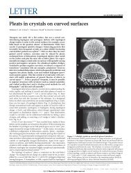
FIG. 2: A surface with negative intrinsic curvature. The two principal curvatures are denoted by κ1 <strong>and</strong> κ2 <strong>and</strong> their product, 

Figure 1.3: A surface with negative Gaussian curvature. The two principal curvatures 

(with dimensions of an inverse length) are denoted by κ1 <strong>and</strong> κ2; their product is the 

Gaussian curvature G(x) = κ1κ2, which is negative in this example. 

the intrinsic curvature, is negative (reproduced from Ref. [1]). 

defect of charge q <strong>and</strong> the background curvature distribution is quadratic in q, hence both vortices <strong>and</strong> anti-vortices 

are repelled from the top of the bump. 

It is our hope to test the existence of this interaction in He films by studying how it competes against the familiar 

1.1.2 Mechanisms of coupling between defects <strong>and</strong> curvature 

confining potential generated by the rotation of the bump. This geometric force exists in a variety of ordered phases 

whose defects interact like a Coulomb gas <strong>and</strong> provides an unexpected coupling between matter <strong>and</strong> geometry. 

Defects in two dimensional monolayers can be modeled as point-like particles 

II. BASIC THEORETICAL IDEAS 

that live in the local tangent plane to the surface <strong>and</strong> cannot escape in the third 

A defect at position r will feel a total potential energy, E(r), given by 

dimension. The defects are sensitive to the Gaussian curvature of the substrate (see 

E(r) 

= V (r) + A(r) 

+ c , (3) 

λ2 � 2 ρ 

m 2 

Fig. 1.3), the latter being an intrinsic property of space that can be probed without 

where m is the mass of 4He, ρ is the superfluid density <strong>and</strong> c is an arbitrary constant. The length λ is defined as 

� 

ever leaving the surface. Experiments � 

λsuch ≡ as those . initiated in the Weitz lab can be (4) 

mω 

described fairly well by approximating the droplets as spheres of constant positive 

The first contribution to E(r), �2ρ m2 V (r), accounts for the interaction of the defect with the curvature (see Fig. 3). The 

second contribution is �ρω 

m A(r), where A(r) is the area within a cup of radius r <strong>and</strong> it is multiplied by the number 

density Gaussian <strong>and</strong> thecurvature. energy quantum A �ω. significant This last term portion generalizes of this (tothesis curved space) addresses the familiar the less parabolic restrictive potential in 

flat space that tries to confine the defect at the center of the bump as a result of the rotation (see Fig. 4). As one varies 

α a second order transition occurs. In fact, Fig. 5 reveals that for α greater than a critical value αc the total energy 

E(r) case assumes of condensed a mexican hat matter shape whose order minima on aissubstrate offset with respect of varying to the top Gaussian of the bump. curvature. Taking a derivative See 

of Eq.(4) with respect to r leads to an implicit equation for the position of the minimum, rm, (or maximum): 

Figures 1.3 <strong>and</strong> 1.4 for examples. 

rm 

λ = sin(θ[rm]) . (5) 

The varying Gaussian curvature of the substrate acts as a source for a one 

where θ(r) is the angle that the tangent at r to the bump forms with the xy plane in Fig. 1a. A simple graphical 

construct allows to solve Eq.(5) by finding the intercept(s) of the sine curve on the RHS with the straight line of slope 

2


body potential V (�x) of purely geometrical origin that controls the equilibrium dis- 

tribution of the defects in the ground state <strong>and</strong> poses constraints on their dynamics. 

These geometric interactions depend crucially on the scalar or vector topological 

charge of the defect <strong>and</strong> on the symmetry of the order parameter. The defect poten- 

tial is a non local function of the Gaussian curvature that can be explicitly determined 

using the ideas <strong>and</strong> methods discussed in this thesis. To make the ideas more con- 

crete, I shall compare the geometric potential felt by vortices in superfluid 4 He on 

curved surfaces to the one experienced by vacancies in crystalline solids grown on 

a curved substrate. The former are topological defects that introduce long distance 

disturbances in the superfluid flow lines. The latter are point defects that arise from 

locally subtracting only one atom from the curved space solid. Despite their obvious 

differences these two objects experience the same geometric potential V (x) that is 

given (apart from multiplicative constants) by the solution of a Poisson-like equation 

∆V (x) = −G(x) (1.1) 

where ∆ is the Laplacian <strong>and</strong> the Gaussian curvature G(x) plays the role of an elec- 

trostatic like background charge. For the bump-like deformation shown in Fig. 1.4, 

the qualitative form of V (x) in Eq.(1.1) can be guessed by appropriately generalizing 

Gauss’s law of electrostatics. (An indented, dimple-like surface is equivalent within 

our model to the one of Fig. 1.4 because the Gaussian curvature is the same). 

Provided there is circular symmetry, the field −∇V (x) (proportional to the 

force on a defect) can be determined as in electrostatics from integrating G(x) over 

a circular patch centered around the top of the bump <strong>and</strong> with radius given by the


(a) 

x 

r 

Figure 1.4: (a) A surface with a bump-like deformation. (b) Top view of (a) showing 

a schematic representation of the positive <strong>and</strong> negative Gaussian curvature as a nonuniform 

background ”charge” distribution that switches sign at a characteristic radius 

r = r0 proportional to the size of the bump. The varying density of + <strong>and</strong> - signs is 

intended to mimic the changing Gaussian curvature in the vicinity of the bump. 

position of the defect. This integral is always positive <strong>and</strong> vanishes only at infinity 

because the Gaussian bump is topologically equivalent to the plane. Hence the defect 

potential V (x) is a monotonically decreasing function of the radial distance <strong>and</strong> both 

vacancies <strong>and</strong> vortices are repelled from the top of the bump where the curvature is 

positive. These defects will not remain trapped in the regions where the curvature 

is most negative, because the net force they experience results from the long range 

(logarithmic) interaction with the Gaussian curvature everywhere on the surface. A 

detailed derivation of these results along with heuristic arguments that make them 

plausible is presented in the following chapters. Here we simply show how these 

results fit in our general conceptual scheme. 

Although they share a common geometrical potential V (x), vacancies <strong>and</strong> 

x 

(b)


vortices are coupled to the Gaussian curvature by two distinct mechanisms that we 

broadly classify as gauge <strong>and</strong> anomalous interactions respectively. The former results 

from a direct coupling between the gradient of the displacement field ui(�x) <strong>and</strong> the 

geometry of the substrate as described by gradients of its height function h(�x). The 

in-plane elastic free energy for a crystal embedded in a gently curved frozen substrate 

can be expressed in terms of the flat space Lamé coefficients µ <strong>and</strong> λ [14] as 

� 

Fc = dS 

� 

µ u 2 ij + λ 

2 u2 � 

kk 

, (1.2) 

where dS is the infinitesimal area element. The strain tensor uij given by 

uij(�x) = 1 

2 [∂iuj(�x) + ∂jui(�x) + Aij(�x)] , (1.3) 

contains an additional term Aij(�x) = ∂ih(�x)∂jh(�x) (compared to its flat space coun- 

terpart) that encodes informations on the geometry of the substrate. This rank two 

tensor resembles the vector potential of electromagnetic theory; an appropriately de- 

fined curl is equal to the Gaussian curvature [15]. A free energy like Eq.(2) has the 

typical structure of the gauge theories often employed to describe condensed matter 

order such as the London theory of a superconductor well below TC. In the super- 

conductor analogy, the Gaussian curvature plays the role of a frozen <strong>and</strong> spatially 

varying external magnetic field. 

The gauge coupling generates a force on each defect which is given by the 

product of the field −∇V (x) <strong>and</strong> the “charge” of the α th point defect Ωα. The corre- 

sponding defect ”strength” Ωα for an isotropic vacancy (interstitial) is given by the 

negative (positive) area change caused by removing (adding) an atom at position xα.


Figure 1.5: An impurity in a crystalline matrix. The large shaded atom causes a local 

dilation of the lattice. The square lattice has been chosen for simplicity, although the 

ground state of a flat two dimensional solid is typically an hexagonal lattice. By 

contrast, a vacancy would correspond to removing the shaded atom from the lattice 

leaving a local compression (reproduced from Ref.[16]). 

The case of substitutional impurities can be treated phenomenologically by choosing 

Ωα according to the characteristic ”size” of the foreign atom introduced in the original 

lattice (see Fig. 1.5); Ωα will hence be allowed to vary continuously in our treatment 

[16]. The coupling constant for this elastic interaction is controlled by the Young’s 

modulus Y = 4µ(µ+λ) 

. As shown in Chapter 5, the resulting force on a vacancy (in- 

2µ+λ 

terstitial) in the outward (inward) radial direction, � fc, has the familiar form of the 

electrostatic interaction between a charge <strong>and</strong> an external field, 

�fc = − Y 

2 Ωα � ∇V (x) . (1.4) 

The tensor Aij(�x) accounts for another key feature of two dimensional crys- 

tals on a curved substrate which is intimately related to the existence of a gauge 

coupling: geometric frustration. In the presence of Gaussian curvature, the elastic


ground state will always be characterized by some strain u G ij(x) <strong>and</strong> stress σ G ij(x) which 

result in a non-vanishing stretching energy, even in the absence of defects. The origin 

of the long range geometric potential V (�x) experienced by vacancies <strong>and</strong> interstitials 

lies in the fact that the local compression or dilation (measured by Ωα) that they 

induce couples to the preexisting isostatic pressure of the stress σ G kk (xα), which is a 

non-local function of the Gaussian curvature. In fact, elastic deformations created 

by the geometric constraint throughout the curved 2D solid are propagated to the 

position of the point defect, xα, by force chains spanning the entire system. Vacan- 

cies, interstitials or impurities atoms can all be viewed as local probes of the stress 

field that, as a first approximation, are unaffected the additional stresses induced by 

their own presence (see Chapter 5). The additional self-energies which are not taken 

into account by this approach are of order Y Ω 2 αG(�x) <strong>and</strong> can be neglected as long as 

the ”size” of these point defects is much smaller than the radii of curvature of the 

substrate. 

By contrast, no geometric frustration exists for a 4 He film on a corrugated 

substrate because its wave function Ψ(x) = A e iθ(x) is defined in a different space from 

the one in which the superfluid is confined. In the ground state of a 4 He film, the 

phase θ(x) is constant throughout the surface <strong>and</strong> the corresponding energy vanishes. 

The free energy, Fs, of a nonrotating superfluid film does not include a geometric 

gauge field. As discussed in Chapter 3, this free energy reads 

Fs = K 

2 

� 

dS g αβ ∂αθ(x) ∂βθ(x) , (1.5) 

where gαβ is the metric tensor of the substrate <strong>and</strong> the coupling constant K = ρs�2 

m4 2 is


expressed in terms of the mass of an 4 He molecule m4 <strong>and</strong> the superfluid mass den- 

sity per unit area ρs. When vortices are introduced into Eq.(4.2), these ”topological 

charges” behave somewhat like electrostatic charges when confined in a bounded ge- 

ometry. Even in the absence of externally imposed supercurrents, position-dependent 

self-energies originate from the broken translational symmetry implied by the presence 

of the boundary or the varying Gaussian curvature. In an electrostatic analogy, each 

charged ”particle” induces polarization charges on the conducting walls (distributed 

according to the shape of the boundary) with which it interacts [17]. On a curved 

substrate, the induced topological charge depends both on the “charge” (quantum of 

circulation) of the vortex <strong>and</strong> on the Gaussian curvature of the surface in which it is 

imbedded. The resulting force, fs is given in terms of the solution of Eq.(1.1) by 

�fs = πK s 2 � ∇V (x) , (1.6) 

where the integer s measures the vorticity of the defect. Unlike the charge Ωα that 

describes the local area deformations in crystals, this topological charge of a vortex 

or anti-vortex must be quantized. A comparison of Eq.(1.4) <strong>and</strong> Eq.(1.6) reveals that 

the geometric forces experienced by vacancies (for which Ωα < 0) <strong>and</strong> vortices or 

anti-vortices in 4 He are indeed the same (apart from multiplicative constants). Note 

however that the dependence on the ”charge” of the point defect, Ωα, is linear in 

Eq.(1.4) whereas the force in Eq.(1.6) depends quadratically on the vortex charge 

s. The mechanism of coupling between curvature <strong>and</strong> vortices in liquid helium is 

qualitatively different from the gauge coupling discussed in the context of curved 

space crystallography <strong>and</strong> in what follows we will refer to it as anomalous coupling.


Figure 1.6: Monte Carlo simulation of curvature induced unbinding of dislocations for 

particles interacting with a Yukawa pair potential on two similar curved substrates 

[18]. The dark <strong>and</strong> light particles in the dislocation core represent a disclination pair. 

The two panels represent c<strong>and</strong>idate ground states that have lower energies than the 

respective configurations without defects. In the left panel, unbound dislocations (i.e. 

disclinations pairs) are oppositely aligned in the radial direction towards the bump. 

In the right panel, dislocation dipoles neutralize their Burger’s vectors by having 

their (opposite) dipole orientation alternate between being pointed towards bumps 

<strong>and</strong> away from saddles. The first scenario is favored for large bump separations. 

Other defects such as disclinations in liquid crystals fit in this classification with both 

types of couplings playing an important role. 

An interesting consequence of geometric frustration in curved crystals <strong>and</strong> 

liquid crystals is the possibility of structural transitions between a defect-free ground 

state to energetically favored configurations where defects nucleate to partially screen 

the Gaussian curvature. Fig. 1.6 shows the result of minimizing the energy of point 

particles interacting via a Yukawa potential <strong>and</strong> constrained to lie on a corrugated 

geometry with two different values of the bump spacing relative to the bump size 

[18]. The two c<strong>and</strong>idate ground states characterized by a ”charge-neutral” set of 

dislocations have lower energies than a frustrated but defect-free hexagonal lattice. 

Both the actual distribution of dislocations <strong>and</strong> the critical aspect ratio of the bumps


necessary to trigger the instability can be calculated from the geometric potential of 

an isolated dislocation, which is a function of both its position <strong>and</strong> the orientation of 

its Burger vector (see Chapter 5). 

1.1.3 Cross-over between 2D <strong>and</strong> 3D physics 

The theoretical framework described in the previous pages applies to very 

thin films of approximately constant thickness which can be treated as two dimen- 

sional systems. It is interesting to study the crossover from the two to three di- 

mensional regime that occurs as the thickness of the layer of material, h, increases. 

Consider for concreteness the case of a nematic shell coating a solid colloidal parti- 

cle on which the nematic molecules are aligned tangentially or a ”double emulsion” 

composed of a nematic liquid coating PVA enriched water droplets in a solution of 

glycerol, PVA <strong>and</strong> water. Experimental investigations of this later system are cur- 

rently underway in the Weitz lab [11]. 

In the mono-layer limit, the baseball like texture reproduced in Fig. 1.2 is 

characterized by four s = 1 

2 

disclinations. However, for thicker shells three dimen- 

sional defect configurations characterized by two pairs of half-hedgehogs at the inner 

<strong>and</strong> outer surface compete with the planar texture discussed previously leading to 

structural transitions above a critical value of hc. The escaped 3D texture is illus- 

trated schematically in the right most panel of Fig. 1.7 where the pair of surface 

half-hedgehogs at the south pole is highlighted by the small circle <strong>and</strong> the center of 

each defect indicated by a dot. For samples between crossed polarizers, the optical 

signature of this transition is a change from the quadrupolar to the bipolar defect


Figure 1.7: Quadrupolar <strong>and</strong> bipolar double-emulsions observed through crossed polarizers. 

In the left panel, the 4 disclinations are visible as 4 two-fold brushes as in 

Fig. 1.2. Each of the two pairs of half-hegehogs is visible in the middle panel as 

a 4-fold brush. Experimental conditions are similar to Fig. 1.2. The right panel 

shows a schematic illustration of a c<strong>and</strong>idate nematic texture escaped in the third 

dimension that is consistent with the image of the bipolar droplet presented in the 

middle panel. Thickness inhomogeneities in the nematic shell are believed to bring 

these defect patterns into the same hemisphere, which allows easy visualization. 

patterns illustrated in Fig. 1.7. 

1.1.4 Outline of the thesis 

This thesis is organized around the themes sketched in the previous sec- 

tions. In Chapter 2 we present a detailed study of liquid crystal order on surfaces 

of varying Gaussian curvature that relies on the geometric potential of an individual 

disclination. The (exact) non-perturbative solution of the Poisson equation by means 

of conformal mappings introduced in this context is an important mathematical in- 

gredient of our approach. In Chapter 3, the crucial distinction between the gauge <strong>and</strong> 

anomalous couplings to the Gaussian curvature is discussed by comparing the physics 

of liquid crystal <strong>and</strong> superfluid films on a corrugated substrate. The mathematical 

description of these two systems is very similar in the plane [1, 2], but this chapter 

reveals remarkable differences on a curved substrate. In Chapter 4 the ground state


of liquid crystal shells is explored including an analysis of the crossover between two 

<strong>and</strong> three dimensional regimes. In Chapter 5, we conclude with a study of the curved 

space crystallography of dislocations, vacancies <strong>and</strong> interstitials <strong>and</strong> impurity atoms. 

Our approach starts from the derivations of the geometric potentials which act on 

these defects <strong>and</strong> proceeds with a discussion of stress relaxation <strong>and</strong> defect unbind- 

ing instabilities in two dimensional crystals on curved substrates. The dynamics of 

dislocation motion on a curved surface is discussed as well.

Chapter 2 

Bond-orientational order on a 

corrugated substrate. 

Based on V. Vitelli <strong>and</strong> D. R. Nelson PRE 70, 051105 (2004). 

16

Chapter 2: Bond-orientational order on a corrugated substrate. 17 


The melting of a two dimensional crystal can occur continuously via two 

second order topological phase transitions characterized by the successive unbinding 

of dislocation <strong>and</strong> disclination pairs. At low temperatures, dislocations are suppressed 

due to their large energy cost, but as the temperature is increased, the entropy gained 

by creating defects overcomes their cost in elastic energy <strong>and</strong> dislocation unbinding 

occurs to reduces the overall free energy of the system [19, 20, 21]. The quasi-long 

range order of the crystal is thus destroyed leading to an hexatic phase that still 

preserves quasi-long range orientational order. This phase can be characterized by 

a complex order parameter with six-fold symmetry. As the temperature is increased 

still further, an additional disclination-unbinding transition occurs <strong>and</strong> the hexatic 

order is finally lost in an isotropic liquid phase [19]. 

Experimental evidence for hexatic order <strong>and</strong> defect-mediated melting has 

been obtained in systems as diverse as free st<strong>and</strong>ing liquid crystal films [22], Langmuir- 

Blodgett surfactant monolayers [23], two-dimensional magnetic bubble arrays [24], 

electrons trapped on the surface of liquid helium [25, 26, 27], two-dimensional colloidal 

crystals [28, 29] <strong>and</strong> self-assembled block copolymers [30]. 

The unbinding of defects in the plane is entropically driven <strong>and</strong> at low tem- 

perature defects are tightly bound. By contrast, on surfaces with non zero (integrated) 

Gaussian curvature, excess defects must be present even at very low temperatures. 

The theory of topological defects in ordered phases confined to frozen topographies 

with positive or negative Gaussian curvature has been investigated previously; see,


e.g., [15, 31, 2]. As a general rule, regions of positive or negative curvature (valleys, 

hills or saddles) lead to unpaired disclinations in the ground state, possibly screened 

by clouds of dislocations. These clouds can in turn condense into grain boundaries 

at low temperature. The predictions of recent studies of crystalline order on a sphere 

[4] have been confirmed in elegant studies of colloidal particles packed on the surface 

of water droplets in oil [3]. Investigations of the physics of defects in curved spaces 

have also been carried out for fluctuating geometries [32, 33, 34, 35]. The dynamics of 

hexatic order on fluctuating spherical interfaces was studied in Ref. [36]. Quenched 

r<strong>and</strong>om topographies in the limit of small deviations from flatness were investigated 

in Ref. [15] . 

In the present work, we investigate topography-driven generation of defects 

on simple frozen surfaces with spatially varying Gaussian curvature whose topology 

does not automatically enforce their presence in the ground state. We study in 

particular a two-dimensional ”bump” with a Gaussian shape <strong>and</strong> dimension large 

compared to the particle spacing. For such a hilly l<strong>and</strong>scape, flat at infinity, the 

geometric control parameter is an aspect ratio given by the bump height divided by 

its spatial extent. Consider a hexatic phase draped over such a bump. For small 

bumps, the ideal hexatic texture is distorted, but there are no defects in the ground 

state. As the aspect ratio is increased, we find that disclination pairs progressively 

unbind at T = 0 in a sequence of transitions occurring at critical values of the aspect 

ratio. The defects subsequently position themselves to partially screen the Gaussian 

curvature. For bumps embedded in surfaces of sufficiently small spatial extent, a


second instability of the smooth ground state needs to be considered. In this case, 

the energy stored in the field can be lowered by generating a single positive defect at 

the center of the bump. Novel effects also arise when the hilly surface is encircled by 

an aligning circular wall that insures a 2π rotation of the orientational order in the 

ground state. In this case, some of the positive defects required to match the curvature 

of the boundary are confined to a hemispherical cup centered on the bump, provided 

the aspect ratio α is larger than a critical value αD. When α is lowered below αD, 

the positive defects originally ”trapped” in the hemispherical cup start undergoing 

a series of sharp ”deconfinement transitions”, as they progressively migrate to new 

equilibrium positions dictated by boundary conditions <strong>and</strong> the finite system size. We 

also suggest possible ground states for periodic arrays of bumps, like those on the 

bottom of an egg carton. 

A natural arena to experimentally study the interplay between geometry 

<strong>and</strong> defects is provided by thin copolymer films on SiO2 patterned substrates [37]. 

Flat space experiments by Segalman et al. have already demonstrated that spherical 

domains in block copolymer films form hexatic phases [30]. 

Our results for hexatics on frozen topographies also apply to other XY- 

like models, as might be appropriate for tilted surface-active molecules on curved 

substrates with interactions which favor alignment. The results are relevant as well to 

two-fold nematic order on frozen topographies. In both cases, we expect qualitatively 

similar defect unbinding transitions, although the equivalence becomes more exact 

in the one Frank constant approximation [38]. Related results have been obtained


recently for order on a torus [39]. Even though the integrated Gaussian curvature 

vanishes, defects appear in the ground state in the limit of fat torii, unless the number 

of degrees of freedom is very large. 

The outline of this paper is as follows. In Section II, the relevant mathemat- 

ical formalism is introduced <strong>and</strong> used to highlight similarities <strong>and</strong> differences between 

defects on surfaces of varying curvature <strong>and</strong> electrostatic charges in a non-uniform 

background charge distribution in flat space. As an example, we calculate the dis- 

torted, but defect-free, ground state texture of a hexatic confined to a surface shaped 

as a ”Gaussian bump” for aspect ratios below the first disclination-unbinding instabil- 

ity. In Section III, we investigate curvature-induced defect formation for an isolated 

bump <strong>and</strong> a periodic array of bumps. In section IV, defect deconfinement is discussed 

<strong>and</strong> in section V various experimental issues related to our analysis are highlighted 

along with some directions for future work. The development of the mathematical 

formalism is largely relegated to Appendices. In Appendix A the Green’s function 

for the covariant Laplacian is derived by means of conformal transformations. In Ap- 

pendix B, we introduce a geometric potential whose source is the Gaussian curvature. 

In Appendix C, we present the general formula for the energy of textures with defects 

in terms of the two functions derived in Appendix A <strong>and</strong> B. We thus explore the 

existence of position-dependent defect self-interactions that arise from the varying 

Gaussian curvature. Finally, boundary effects are discussed in Appendix D.


2.2 Hexatic order on a surface 

2.2.1 Electrostatic analogy 

The free energy for hexatic degrees of freedom embedded in an arbitrary 

frozen surface can be written as 

F = KA 

2 

� 

dA Dαn β (u)D α nβ(u) , (2.1) 

where u = {u1, u2} is a set of internal coordinates, n(u) is a unit vector in the tangent 

plane, Dα is the covariant derivative with respect to the metric of the surface <strong>and</strong> dA is 

the infinitesimal surface area [33, 32, 35, 40]. The generalization to systems with a p- 

fold symmetry is straightforward provided that the one Frank constant approximation 

is used <strong>and</strong> the consequences of the uniaxial coupling neglected [38]. This choice of 

free energy implies that the minimal energy configuration will be given locally by 

neighboring n(u) vectors which differ only by parallel transport. The curvature of the 

surface induces ”frustration” in the texture. In fact, by Gauss’ ”Theorema egregium” 

[41, 42], tangent vectors parallel transported along a closed loop are rotated by an 

amount equal to the Gaussian curvature integrated over the enclosed area. On a 

sphere, for example, the hexatic ground state always has twelve excess disclinations 

as a result of this frustration [31, 12]. More generally, the sum of the topological 

charges on any closed surface is equal to the integrated Gaussian curvature. 

By introducing a local bond-angle field θ(u), corresponding to the angle 

between n(u) <strong>and</strong> an arbitrary local reference frame, we can rewrite the hexatic free


energy introduced in Eq.(3.1) as: 

F = 1 

2 KA 

� 

dA g αβ (∂αθ − Aα)(∂βθ − Aβ) , (2.2) 

where dA = d 2 u √ g, g is the determinant of the metric tensor gαβ <strong>and</strong> Aβ is the spin- 

connection whose curl is the Gaussian curvature G(u) [40, 42]. The spin connection 

can be viewed as a ”geometric vector potential”. A free energy like Eq.(2) also 

describes the charged Cooper pairs implicit in the London theory of a superconductor 

well below TC. In the superconductor analogy, the Gaussian curvature plays the role 

of a (spatially varying) external magnetic field. For the problem considered here, 

however, there are interesting new nonlinear effects associated with spatial variations 

in the metric. 

A detailed analysis of the free energy of Eq.(2.2) for a bumpy surface with 

free <strong>and</strong> circular boundary conditions is presented in Appendices (C) <strong>and</strong> (D). Here 

we only sketch the main steps <strong>and</strong> conclusions. The free energy can be readily con- 

verted into a Coulomb gas model by using the relation 

γ αβ ∂α(∂βθ − Aβ) = s(u) − G(u) ≡ n(u) , (2.3) 

where γ αβ is the covariant antisymmetric tensor, G(u) is the Gaussian curvature <strong>and</strong> 

s(u) ≡ 1 �Nd √ 

g i=1 qiδ(u − ui) is the disclination density with Nd defects of charge qi at 

positions ui. The final result is an effective free energy whose basic degrees of freedom 

are the defects themselves [35, 4]: 

F = KA 

2 

� 

� 

dA 

dA ′ n(u) Γ(u, u ′ ) n(u ′ ) , (2.4)


where n(u) is defined in Eq.(E.18). The Green’s function Γ(u, u ′ ) is calculated (see 

Appendix A) by inverting the Laplacian defined on the surface 

Γ(u, u ′ � � 

1 

) ≡ − 

∆ uu ′ 

, (2.5) 

<strong>and</strong> we have suppressed for now defect core energy contributions which reflect the 

physics at microscopic length scales. Eq.(E.19) can be understood by analogy to two 

dimensional electrostatics, with the Gaussian curvature G(u) (with sign reversed) 

playing the role of a non-uniform background charge distribution <strong>and</strong> the topolog- 

ical defects appearing as point-like sources with electrostatic charges equal to their 

topological charge qi. As a result, the defects tend to position themselves so that 

the Gaussian curvature is screened: the positive ones on peaks <strong>and</strong> valleys <strong>and</strong> the 

negative ones on the saddles of the surface. However, this analogy does neglect 

position-dependent self-interactions [43], but since these are quadratic in the charge 

they are negligible for hexatics. Hence positive disclinations of minimal topological 

charge qi = 2π 

6 

continue to be attracted to positive curvature (see Appendix C). 

More generally, we can consider p-fold symmetric order parameters with 

minimum charge defects ± 2π. 

The case p = 1 corresponds to tilt order of absorbed 

p 

molecules <strong>and</strong> p = 2 describes 2D nematics. The cases p = 4 <strong>and</strong> p = 6 describe 

tetradic <strong>and</strong> hexatic phases respectively [12]. Strictly speaking, Eq.(1) only describes 

the cases p = 1 <strong>and</strong> p = 2 in the one-Frank-constant approximation [38]. Most of 

our discussion focuses on topography-driven transitions on a model surface shaped 

like a bell curve or ”Gaussian bump” (see Fig. 2.1), but the same mathematical 

approach can be readily carried over to study arbitrary surfaces of revolution that


Figure 2.1: (a) The vector field n is confined to a surface shaped as a Gaussian. 

(b) Top view of (a) showing a schematic representation of the positive <strong>and</strong> negative 

Gaussian curvature as a background ”charge” distribution that switches sign at r = 

r0. Note that, according to the electrostatic analogy, a positive (negative) distribution 

of Gaussian curvature corresponds to negative (positive) topological charge density. 

are topologically equivalent to the plane. Furthermore, we do not expect the results 

of this analysis to depend qualitatively on the azimuthal symmetry of the surface, 

which is assumed purely for reasons of mathematical convenience. 

Points on our model surface embedded in three dimensional Euclidean space 

are specified by a three dimensional vector R(r, φ) given by 

⎛ 

⎞ 

⎜ r cos φ 

⎜ 

R(r, φ) = ⎜ 

r sin φ 

⎝ 

h exp 

� 

− r2 

2r 2 0 

⎟ , (2.6) 

⎟ 

� ⎠ 

where r <strong>and</strong> φ are plane polar coordinates in the xy plane of Fig. 2.1. It is useful 

to characterize the deviation of the bump from a plane in terms of a dimensionless


7 

6 

5 

4 

3 

2 

1 

l(r/r0) 

r/r0 

0.5 1 1.5 2 2.5 3 

Figure 2.2: Plot of l( r 

r 

) as a function of the dimensionless radial coordinate r0 r0 for 

α = 1, 2, 3, 4. The arrow is oriented in the direction of increasing α. 

aspect ratio 

α ≡ h 

r0 

. (2.7) 

The two orthogonal tangent vectors tr ≡ ∂R 

∂r <strong>and</strong> tφ ≡ ∂R can be normalized to define 

∂φ 

the Vierbein (orthonormal basis vectors) Er <strong>and</strong> Eφ respectively. The components of 

the spin connection introduced in Eq.(2.2) are given by Aα = Er · ∂αEφ [40, 42]. This 

leads to a vanishing radial component Ar <strong>and</strong> 

Aφ = − 1 

� l(r) , (2.8) 

where the important α-dependent function l(r) (see Fig. 2.2) is defined by 

l(r) ≡ 1 + α2 r 2 

r 2 0 

� 

exp − r2 

r2 � 

0 

, (2.9)


<strong>and</strong> it is equal to the radial component of the diagonal metric tensor, gαβ, 

⎛ 

⎜l(r) 

gαβ = ⎝ 

0 

0 r2 ⎞ 

⎟ 

⎠ . (2.10) 

Note that the gφφ entry is equal to the flat space result r 2 in polar coordinates while 

grr = l(r) is modified in a way that depends on α but tends to the plane result grr = 1 

for small <strong>and</strong> large r, as illustrated in Fig. 2.2. 

The Gaussian curvature for the bump is readily found from the eigenvalues 

of the second fundamental form [44], 

Gα(r) = α2 r2 

− 

r e 2 0 

r2 0 l(r) 2 

� 

1 − r2 

r2 � 

0 

. (2.11) 

Note that α controls the order of magnitude of G(r) <strong>and</strong> that G(r) changes sign at 

r = r0 (see Fig. 2.1b). The integrated Gaussian curvature ∆G(r) inside a cup of 

radius r centered on the bump is 

∆G(r) = 2π 

� 

1 − 1 

� 

� 

l(r) 

, (2.12) 

which vanishes as r → ∞. Eq.(2.12) also shows that the positive Gaussian curvature 

enclosed within the radius r0 (see Fig. 2.1) approaches 2π for α ≫ 1, half the 

integrated Gaussian curvature of a sphere. 

2.2.2 Defect free texture 

For small values of the aspect ratio α, the minimal energy texture for the 

hexatic will be free of defects. The ground state configuration θo(u) satisfies the 

differential equation 

DαD α θ0 − D α Aα = 0 , (2.13)


Figure 2.3: Projected ground state texture for an XY model on the bump, with the 

boundary condition that the vector field is parallel to the y-axis at infinity. The two 

insets show the defect pairs suggested by two regions of large frustration, which lie 

close to a circle of radius r0. 

which results from minimizing the free energy in Eq.(2.2) with respect to the field θ(u) 

for fixed Aα. When expressed in terms of the coordinates in Eq.(2.6), the solution of 

Eq.(2.13) reads: 

θo(u) = −φ + c , (2.14) 

where c is an arbitrary constant. The smooth ground state texture is thus obtained 

if the director n forms an angle θo(u) = −φ + c with respect to the spatially varying 

basis vector Er. Note that a solution of the form θo(u) = c represents a defect of 

charge q = 2π in this ”rotating” system of coordinates. 

As an illustration, consider the projection on the plane of the minimal en- 

ergy texture of an XY model (p = 1) as shown in Fig. 2.3. The arrows represent 

the orientation of tilted molecules on this surface in the one Frank constant approxi- 

mation. The field clearly displays strong frustration along a direction determined by


the choice of the constant c in Eq.(2.14). If the bump is positioned within two very 

distant walls parallel to the y-axis which impose tangential boundary conditions on 

the molecular tilts, the ”preferred” direction will be along ˆy 1 . The texture displayed 

in Fig. 2.3 can be interpreted as resulting from embryonic pairs of defect dipoles 

along the line x = 0. The distortion energy F0 of this ground state is given by: 

F0 = 1 

2 KA 

� 

dA g αβ (∂αθo − Aα)(∂βθo − Aβ) . (2.15) 

This expression can be evaluated for an infinitely large system by using Eq.(2.14) <strong>and</strong> 

the explicit form of the spin connection derived in Section 2.2.1, with the result: 

� ∞ 

� 

1 − 

F0 = πKA dr 

� �2 l(r) 

r � l(r) 

. (2.16) 

0 

It follows from Eq.(2.16) that the ground state energy is a monotonically increasing 

function of the aspect ratio, proportional to α 4 for small α. As we shall see, for large 

enough α, it can be energetically preferable to reduce this energy by introducing 

defect pairs into the texture. It is convenient to rewrite Eq.(2.15) in terms of the 

Gaussian curvature G(r) <strong>and</strong> the Green function Γ(u, u ′ ) discussed in Appendix A 

[40] 

F0 = KA 

2 

� 

� 

dA 

dA ′ G(u) Γ(u, u ′ ) G(u ′ ) . (2.17) 

This result is what one obtains by setting all qi = 0 in Eq.(E.19). The details of the 

mathematical derivation are relegated to Appendix C. 

Although this result correctly represents the zero temperature limit of the 

vector model, corrections may be appropriate to describe the physics of ordered phases 

1 In case distant walls are present, the free solution of Eq.(2.14) is slightly modified to account for the 

new boundary conditions. This is accomplished by the method of images or conformal transformations [45].


at finite temperature. ”Spin-wave” excitations (i.e., quadratic fluctuations of the 

order parameter about the ground state texture) can be accounted for by integrating 

out the longitudinal fluctuations θ ′ (u) around the ground state configuration θo(u). 

By letting θ = θ0 + θ ′ in Eq.(2.2) <strong>and</strong> using Eq.(E.18) we obtain [32, 35]: 

F = F0 + 1 

2 KA 

� 

dA g αβ ∂αθ ′ ∂βθ ′ , (2.18) 

The longitudinal variable θ ′ (u) appears only quadratically in F <strong>and</strong> the trace over 

θ ′ (u) can be explicitly performed with the result [46]: 

� 

Dθ ′ e − βKA 2 

where FL is the Liouville action, 

� 

βFL = c 

dA − KA 

24 

� 

R dA g αβ ∂αθ ′ ∂βθ ′ 

� 

dA 

= e −βFL , (2.19) 

dA ′ G(u) Γ(u, u ′ ) G(u ′ ) . (2.20) 

The first term in this expression is a constant proportional to the fixed surface area 

of the frozen topography <strong>and</strong> will be suppressed in what follows. The remaining term 

causes a shift in the coupling constant appearing in Eq.(2.17) from KA to K ′ A = 

KA − kBT 

12π [32, 35]. This ”entropic” correction to the coupling constant KA at finite 

temperature also arises when defects are present. 

The energy in Eq.(2.17) represents an intrinsic, irreducible energy cost of 

geometric frustration for textures without defects. As we shall see, defects can reduce 

this frustration. However, for small values of α the energy cost of this frustration 

will still be lower than the core energies associated with the creation of the unbound 

defects <strong>and</strong> the work necessary to tear them apart.


2.2.3 Energetics of defect pairs on a Gaussian bump 

A quantitative underst<strong>and</strong>ing of the energetics of defects on a fixed topog- 

raphy is essential to calculate the critical value(s) of the aspect ratio above which 

defect-unbinding becomes energetically favorable. The first step is to calculate the 

Green’s function Γ(u, u ′ ) that governs the ”coulombic” interaction among defects <strong>and</strong> 

between each defect <strong>and</strong> the Gaussian curvature. The inversion of the curved space 

Laplacian can be more easily accomplished by employing a set of ”isothermal coor- 

dinates”, such that the resulting Green’s function reduces to the familiar logarithm 

of two dimensional electrostatics. As shown in Appendix A the final result in terms 

of the original polar coordinates reads: 

Γ(u, u ′ ) = − 1 

4π ln[ℜ(r)2 + ℜ(r ′ ) 2 

− 2ℜ(r)ℜ(r ′ ) cos(φ − φ ′ )] + c , (2.21) 

where the function ℜ(r) can be thought of as a radial coordinate in the conformal 

plane resulting from adopting an isothermal set of coordinates (see Appendix A) 

ℜ(r) = r e − R ∞ 

r 

dr ′ 

r ′ 

“√ ” 

l(r ′ )−1 

, (2.22) 

<strong>and</strong> l(r) is the α-dependent function introduced in Eq.(2.9). The constant c depends 

on the physics at short distances, which is discussed in Appendix A. 

The Green function in Eq.(2.21) corresponds to free boundary conditions 

at infinity <strong>and</strong> preserves the cylindrical symmetry of the metric. It differs from 

the familiar result in flat space by a non-linear radial stretch corresponding to a 

smooth deformation of the bump into a flat disk. This Green’s function determines an


attractive interaction for the defect dipole pair. However, the Gaussian curvature of 

the bump also generates a geometric potential that tries to pull the disclination dipole 

apart. This geometric interaction arises by combining cross terms between s(u) <strong>and</strong> 

G(u) in Eq.(E.19) with the position dependent self-interactions derived in Appendix 

C. The resulting interaction FG between defects <strong>and</strong> the Gaussian curvature takes 

the simple form 

Nd � 

FG = KA qi 

i=1 

where the geometrical potential V (u) is defined as 

� 

V (u) ≡ − 

� 

1 − qi 

� 

V (ui) , (2.23) 

4π 

dA G(u ′ ) Γ(u, u ′ ) . (2.24) 

The minus sign in front of this geometric potential insures that defects of topological 

charge between zero <strong>and</strong> 4π are attracted by regions of positive Gaussian curvature 

[43]. For defects with a large topological charge of q > 4π, the sign of the geometric 

interaction, FG, is reversed <strong>and</strong>, <strong>and</strong> defects of either sign are pushed away from the 

bump. This scenario does not affect the geometry-driven defect formation discussed 

in this paper that relies on disclinations whose charge is well below 4π. However, as 

a result of the position-dependent self interactions, FG is no longer symmetric under 

the change q → −q, as one would expect on the basis of the electrostatic analogy. The 

effect of this asymmetry is small for hexatic order but it increase for liquid crystals 

with p-fold order parameter, as p decreases (see Ref. [43], <strong>and</strong> references therein). 

Gauss’ law generalized to curved surfaces (see Appendix B) insures that the 

geometric force experienced by a defect of charge q with radial coordinate r will be 

determined only by the net curvature enclosed in a circle of radius r centered on the


top of the bump. The resulting ”electric field” is radial as expected from electrostatics 

<strong>and</strong> is proportional to the gradient of the geometric potential, which for a Gaussian 

bump takes the form (see Appendix B) 

� ∞ 

dr 

V (r) = − 

r 

′ 

r ′ 

�� 

l(r ′ ) − 1 

. (2.25) 

For small values of the aspect ratio α the potential in Eq.(2.25) can be approximated 

by 

V (r) ≈ − α2 r2 

− 

r e 2 0 

4 

. (2.26) 

The resulting force is linear for small r (i.e. near the top of the bump) <strong>and</strong> decays like 

r2 

− 

r e 2 0 for r ≫ r0. As the aspect ratio α increases, the force generated by the curvature 

can overcome the attractive force binding the defect pair which varies logarithmically 

for short distances. As a result, oppositely charged defects that were originally tightly 

bound can be separated. 

This argument, however, neglects another complication resulting from the 

curvature of the surface: as the aspect ratio is increased, the Green’s function Γ(u, u ′ ) 

in Eq.(2.21) <strong>and</strong> hence the force binding the defects together also increases. We 

illustrate this point in Fig. 2.4 for the special case of a positive defect pinned right 

on top of the bump <strong>and</strong> a negative one free to move downhill at r. Upon invoking 

Equations (E.19) <strong>and</strong> (2.21), the potential binding the pair, Vpair (r), can be written 

down exactly as: 

Vpair (r) = KA q2 2π ln 

� 

r 

� 

a 

− KA q2 � ∞ 

dr 

2π 

′ 

r ′ 

r 

+ 2q 2 Ec 

�� 

l(r ′ ) − 1 

. (2.27)


dr 

+ 

+ 

- 

Rz(r) - 

Figure 2.4: Effect of changing the aspect ratio of the bump on the work needed to pull 

apart two oppositely charged defects. Positive <strong>and</strong> negative defects are represented by 

open circles with their sign printed. The line elements corresponding to the projected 

length dr for the two aspect ratios are shown. 

The first term is the flat space Green’s function <strong>and</strong> we have added two disclination 

core energies. The last term represents a ”curvature correction” that has the same 

functional form of the geometric potential in Eq.(2.25), but it represents a distinct 

contribution to the total free energy. As discussed in Appendix B, the pair potential 

energy, Vpair (r), can be understood by applying a generalized Gauss’ Law to the bump 

to determine a force which is equal to − q2 

. The potential follows by integrating 

2πr 

this force along the bump with the length element dr � l(r). Although the force is 

independent of the aspect ratio, the length element grows with α (see Fig. 2.4), which 

makes the pair more energetically bound for larger values of α. A careful calculation 

of these effects (including the contribution associated with the position-dependent 

self-energies) reveals that the geometric force still overcomes the binding interaction 

r


for sufficiently large values of α. 

An estimate of the critical value of α for which the dipole unbinds can 

be obtained by comparing the minimal free energy of the smooth frustrated field 

arising from Eq.(2.17) with the free energy in the presence of defects. The latter, as 

follows from Eq.(E.19), is composed of three contributions: the interactions among 

the defects, the interaction between the defects <strong>and</strong> curvature as given by Eq.(2.23) 

<strong>and</strong> the Gaussian curvature self-interaction. The latter is equal to the minimal free 

energy of the smooth frustrated field <strong>and</strong> is renormalized at finite temperature in 

the same way. (Associated with the cutoff is a microscopic core energy, Ec, that we 

expect to be independent of the defect position on the bump, as long as the radius 

of curvature is much greater than any microscopic length scale.) The remaining two 

contributions are not renormalized by thermally induced spin wave fluctuations [35]. 

As shown in Appendix C, the difference in free energy of a defected texture described 

by Eq.(E.19) relative to the defect-free result Eq.(2.17) can be written as: 

∆F (α) 

KA 

Nd � 

+ 

i=1 

qi 

= 1 

2 

Nd Nd � 

i=1 

� 

qiqjΓa(ri, φi, rj, φj) 

j�=i 

� 

1 − qi 

� 

V (ri) + 

4π 

Ec 

KA 

Nd � 

i=1 

q 2 i . (2.28) 

where we have assumed overall charge neutrality for the defect configuration. The 

subscript in Γa indicates that a constant microscopic core radius a has been absorbed 

in the definition of the Green function so that the argument of the logarithm in 

Eq.(2.21) becomes dimensionless, as in Eq.(C.21), 

Γa(ri, φi, rj, φj) = Γ(ri, φi, rj, φj) + 1 

ln a . (2.29) 

2π


This microscopic cutoff a corresponds to a constant core radius for each defect <strong>and</strong> 

it is of the order of the spacing between the microscopic degrees of freedom. The 

sum of microscopic core energies in the fourth term of Eq.(2.28) needs to be fixed 

phenomenologically or from models that go beyond simple elasticity theory [47]. Note 

that both Γa(ri, φi, rj, φj) <strong>and</strong> V (r) depend on α. If α becomes sufficiently large so 

that ∆F is less than zero, one or more disclination dipoles unbind in the hexatic phase 

at a sequence of critical values αci . The analogous defects in XY-model textures of 

tilted liquid crystal molecules would be +/− vortex pairs. 

2.3 Curvature induced defect generation 

2.3.1 Onset of the defect-dipole instability 

If a dipole is created, say, along the line r = r0 of zero Gaussian curvature, 

the positive disclination will be pulled towards the center by the positive curvature 

while the negative one will be repelled into the region of negative curvature. The net 

result is a reduction of the total free energy of the order of the depth of the potential 

well since the logarithmic binding energy is approximately constant compared to the 

geometric potential. An approximate analytical treatment is obtained by assuming 

that the positive defect sits right at the center of the bump <strong>and</strong> the negative one at a 

distance of the order of r0. The validity of this approximation scheme can be checked 

by numerically minimizing the energy with respect to the position of the defects, as 

discussed in Section (2.3.2). We assume charge neutrality so that the two defects 

have equal <strong>and</strong> opposite topological charges of magnitude q. For order parameters


V(r/r0 ) 

0 

-0.5 

-1 

-1.5 

-2 

-2.5 

-3 

-3.5 

0.25 0.5 0.75 1 1.25 1.5 1.75 2 

Figure 2.5: Geometric potential V (r/r0) as a function of the dimensionless ratio of r 

<strong>and</strong> r0 for α = 1, 2, 3, 4, 5. Note that | V (r) |≪ | V (0) | for r � r0. The arrow points 

in the direction of increasing α. 

with a p-fold symmetry, the minimal topological charge is q = 2π. 

The approximate 

p 

free energy cost to generate this defect pair then follows from Equations (2.25),(2.27) 

<strong>and</strong> (2.28): 

∆F (α) 

KA 

r/r0 

≈ q2 

� � 

r 

� � � 

ln + V (r) + q 1 − 

2π a 

q 

� 

V (0) 

4π 

� 

− q 1 + q 

� 

2 Ec 

V (r) + 2q . (2.30) 

4π 

KA 

The internal consistency of the formalism can be checked by investigating the limit 

r → a. As the negative defect approaches the positive one at the center of the bump, 

we have V (a) ≈ V (0) <strong>and</strong> the energy tends to the expected flat space result 2q 2 Ec. 

The equilibrium position of the negative defect turns out to be for r equal 

to a few r0, so the terms containing V (r) in Eq.(2.30) can be dropped as a first 

approximation because V (r) decays exponentially (see Fig. 2.5): 

∆F (α) 

KA 

≈ q2 

2π ln 

� 

r 

� � 

+ q 1 − 

a 

q 

� 

2 Ec 

V (0) + 2q . (2.31) 

4π 

KA


V(0) 

0 

-1 

- 2 

- 3 

- 4 

- 5 

- 6 

1 2 3 4 5 

Figure 2.6: Plot of the geometric potential evaluated at the center of the bump, V (0), 

for aspect ratios α between 0 <strong>and</strong> 5. The continuous line is plotted using the exact 

form of V (r) while the dashed line is obtained from the low α expansion given in 

Eq.(2.26). 

To estimate the critical value of the aspect ratio for which the first dipole unbinds, 

let r ∼ r0 <strong>and</strong> solve for αc in Eq.(2.31). Because a different choice for the core energy 

Ec can be accounted for by rescaling the core size a in Eq.(2.31), the condition for 

unbinding is 

with 

If we know Ec 

KA 

|V (0)| > 

2q 

(4π − q) ln 

� 

r0 

a ′ 

� 

, (2.32) 

a ′ = a e 

− 4πEc 

K A . (2.33) 

<strong>and</strong> r0 

a , the critical aspect ratio αc can be obtained from inspection 

of Fig. 2.6 where V (0) is plotted as a function of α. The Taylor expansion of V (r) 

derived in Eq.(2.26) gives V (0) ≈ − α2 

4 

to leading order in α. Inspection of Fig. 2.6 

α


shows that this approximation works sufficiently well even for aspect ratios of order 

unity. Upon substituting for V (0) into Eq.(2.32), we obtain an estimate of how αc 

depends on r0 

a ′ : 

α 2 c ≈ 

≈ 

8q 

(4π − q) ln 

� 

r0 

a ′ 

� 

� 

8q 

� � 

r0 

ln + 

(4π − q) a 

4πEc 

� 

. (2.34) 

KA 

Note that a critical height hc = αcr0 for defect unbinding is predicted for fixed r0 

a ′ 

with defect charge q = 2π 

p 

relation is tested in Section 2.3.2. 

for all integer values of p. The validity of this approximate 

The continuum theory adopted here is valid in the limit r0 ≫ a. If Ec can 

be neglected compared to KA, the defect unbinding instability is triggered when the 

energy gain derived from letting the defects screen the Gaussian curvature (approx- 

imately given by qV (0)) overcomes the work needed to pull them apart a distance 

r0. This work, of order q2 

2π ln � � 

r0 

r0 

, increases very slowly with large , hence the con- 

a 

a 

tinuum approximation can be satisfied while keeping the work finite. Note that the 

result does not depend on the size of the system R because we assume overall discli- 

nation charge neutrality <strong>and</strong> the assumption that R ≫ r0. In this limit, boundary 

effects can be ignored provided that they do not impose a topological constraint on 

the phase of the order parameter. An aligning outer wall in a circular hexatic sample, 

for example, would force the bond angle field to rotate by 2π, leading to six defects in 

the ground state even in flat space. The interesting physics which results is addressed 

in Section 2.4.


2.3.2 Numerical investigation of defect-unbinding transitions 

The disclination unbinding transitions can be investigated more quantita- 

tively by minimizing numerically ∆F (α) in Eq.(2.28) with respect to the positions of 

the defects. The aspect ratio above which ∆F (α) becomes negative corresponds to 

the threshold value αc (analogous to a first order transition) for which the singular 

field is energetically favored with respect to the smooth texture of Fig. 2.3. We 

emphasize that the energy l<strong>and</strong>scape can have two minima. The first occurs when 

two oppositely charged defects form a closely bound dipole (with separation of the 

order of the cutoff a) <strong>and</strong> hence annihilate each other leaving a smooth texture. The 

second minimum corresponds to an unbound pair (with separation of a few r0) <strong>and</strong> 

it disappears when the geometric force is too weak to overcome the binding force of 

the pair. This scenario occurs for a finite value of α characteristic of the geometry 

of the substrate above which the formation of an unbound dipole is possible, albeit 

energetically unfavored (see Fig. 2.7). As α is increased above αc, the smooth-texture 

minimum becomes metastable <strong>and</strong> the unbinding of a defect pair is the most likely 

scenario. 

It is useful to parameterize ∆F (α) in terms of the dimensionless radial co- 

ordinates ¯ri ≡ ri . The geometric potential is defined in Eq.(A.9) as a function of ¯ri, 

r0 

V (r) ≡ ˜ Vα( r ), where 

r0 

� ∞ 

˜Vα(x) 

dy 

�� 

= − 

1 + α2y2 exp(−y2 ) − 1 

x y 

. (2.35) 

In order to write the defect-defect interaction in terms of the dimensionless radial


- 0.15 

- 0.2 

- 0.25 

- 0.3 

0.5 

1 

1.5 

Figure 2.7: Plot of ∆F/KA versus x1 <strong>and</strong> x2 the positions of the negative <strong>and</strong> pos- 

itive defects respectively in units of r0, for α = 1.2. A constant energy offset equal 

to − q2 

2π ln � r0 

a ′ 

� 

has been neglected. The metastable minimum at x1 � 1.3 r0 <strong>and</strong> 

x2 � 0.2 r0 corresponds to an unbound pair (see Fig. 2.8a). As α is decreased 

further the energy barrier that separates this minimum from the smooth texture solution 

(corresponding to x1 approaching x2) disappears <strong>and</strong> the two opposite defects 

annihilate. 

2 

2.5 

coordinate ¯ri, we introduce a new function ˜ ℜ(¯ri) defined by 

˜ℜ(¯ri) ≡ ri 

exp[V (ri)] = ri 

r0 

= ℜ(ri) 

r0 

r0 

� 

exp ˜Vα 

� ri 

r0 

0.1 

�� 

0.2 

, (2.36) 

where Eq.(A.8) was used in the last step. We can now transform Γa(¯ri, φi, ¯rj, φj) by 

eliminating ℜ(ri) in favor of ˜ ℜ(¯ri). Thus we have using Equations (C.21) <strong>and</strong> (A.12) 

Nd 

Nd 

� 

� 

− qiqjΓa(ri, φi, rj, φj) = − qiqjΓ(¯ri, φi, ¯rj, φj) 

j�=i 

+ 1 

2π 

j�=i 

Nd � 

i=1 

q 2 i ln( r0 

) , (2.37) 

a 

where we have exploited charge neutrality <strong>and</strong> Eq.(C.22). The free energy minimized


� 

∆F 

with respect to the positions of the defects, min 

to Eq.(2.28), as 

where 

� � 

∆F 

min 

KA 

= f(α) + 1 

4π 

f(α) ≡ min [ 1 

2 

+ 

Nd � 

qi 

i=1 

Nd � 

j�=i 

Nd � 

i=1 

KA 

q 2 i ln 

� 

, can now be written, according 

� 

r0 

a ′ 

� 

qiqjΓ(¯ri, φi, ¯rj, φj) 

, (2.38) 

� 

1 − qi 

� 

V (¯ri)] . (2.39) 

4π 

Note that in the second term in Eq.(2.38) the core energy of each defect has been 

absorbed in the modified core radius a ′ , as defined in Eq.(2.33). This generates an 

energy cost for unbinding that can be overcome if f(α) assumes sufficiently large 

negative values. Hence it is sufficient to study numerically how ∆F (α) varies as a 

function of a single parameter, eg. r0 

a ′ . As an illustration of this approach, we study 

explicitly the unbinding of one <strong>and</strong> two disclinations pairs leading to the ground states 

represented schematically in Fig. 2.8. The smooth ground state becomes unstable 

to the formation of one defect dipole first. The critical aspect ratio above which this 

scenario occurs can be determined with the aid of Fig. 2.9 where the function f(α) 

introduced in Eq.(2.39) is plotted as a function of the aspect ratio. From Eq.(2.38) 

we see that αc1 is determined by 

f(αc1) = − q2 

2π ln 

� 

r0 

a ′ 

� 

. (2.40) 

For r0 

a ′ = 10 4 <strong>and</strong> q = 2π 

6 , we obtain a critical aspect ratio αc1 ≈ 3.2. As a comparison, 

the approximate condition derived in Eq.(2.32) gives αc1 ≈ 3 when used in conjunction


(a) 

(b) 

+ 

r 0 

- + + 

- 

Figure 2.8: The equilibrium defects positions are illustrated schematically in the case 

of one (a) <strong>and</strong> two dipoles (b). We assume free boundary conditions at infinity, as in 

Fig. 2.3, so that the effect of image charges can be neglected. 

with Fig. 2.6. The rougher estimate in Eq.(2.34) leads (for q = 2π 

6 ) to αc1 ≈ 2.6. This 

discrepancy is easily understood considering that Eq.(2.34) was derived by means of 

a low α expansion. The critical aspect ratio αc1 is too low for the two-dipole defect 

configuration to become energetically favorable with respect to the smooth ground 

state. Indeed, inspection of Fig. 2.10 reveals that the critical aspect ratio αc2 for 

which the ”two-dipole instability” sets in is approximately equal to 3.6 for the same 

choice of parameters used in the single pair case. Note that, in the presence of two 

dipoles, the energy cost arising from the second term in Eq.(2.38) is twice as large 

because there are four defects rather than two. However, for α � 4.2 generating 

two dipoles becomes more energetically favored than a single dipole (see Fig. 2.11). 

The approach illustrated here can be used to calculate a cascade of defect unbinding 

r 0 

x 

-


0 

f(!) 

- 1 

- 2 

- 3 

- 4 

2 3 !c1 4 5 

Figure 2.9: Plot of f(α) versus the aspect ratio α obtained by minimizing over the 

single-dipole defect configuration represented schematically in Fig. 2.8a. As discussed 

in the text, the first unbinding transition occurs when f(αc1) is equal to − q2 

2π ln � r0 

a ′ 

� 

. 

The value αc1 is indicated by the dashed line for r0 

a ′ = 104 <strong>and</strong> q = 2π . Note that no 

6 

minimum (corresponding to an unbound pair) exists for α less than 1 (approximately), 

hence the curve cannot be continued to the origin (see Fig 2.7). 

instabilities at critical aspect ratios αci 

involving higher number of dipoles <strong>and</strong> their 

equilibrium configurations in the ground state. Note that the unbinding eventually 

stops since the integrated Gaussian curvature in the top cup cannot exceed 2π. We 

expect the qualitative features of our analysis to be independent of the exact shape 

of the bumpy substrate although the specific values αci 

! 

depend on the geometry <strong>and</strong> 

the choice of the microscopic parameters a <strong>and</strong> Ec. Finally, we emphasize that the 

curvature-induced unbinding is similar to a first order transition <strong>and</strong> occurs for rather 

pronounced deviations from flatness (ie. large α).


0 

f(!) 

- 1 

- 2 

- 

- 

- 

- 

- 

3 

4 

5 

6 

7 

!c2 

2 3 4 5 

Figure 2.10: Plot of f(α) versus the aspect ratio α obtained by minimizing the twodipole 

defect configuration represented schematically in Fig. 2.8b . The second 

unbinding transition occurs when f(αc2) is equal to − q2 

π ln � r0 

a ′ 

� 

. The value αc2 is 

indicated by the dashed line for r0 

a ′ = 104 <strong>and</strong> q = 2π (compare with Fig. 2.9). 

6 

2.3.3 Single vortex instability 

The unbinding of defect pairs may not be the most likely scenario if the size 

of the system R is sufficiently small. In this case, the creation of a single vortex at 

the center of the bump may become energetically favorable for lower aspect ratios 

than required by the defect dipole instability. The equation for the bond angle field 

θs(u) for a single defect of charge q at the center of the bump is given by: 

θs(φ) = 

� 

q 

� 

− 1 φ , (2.41) 

2π 

where the bond angle is measured with respect to the rotating basis vectors corre- 

sponding to the polar coordinates discussed in Section 2.2.2. Upon substituting θs(φ) 

in Eq.(2.2) <strong>and</strong> subtracting the free energy F0 corresponding to the defect-free texture 

!


2 

1 

0 

- 1 

- 2 

- 3 

!F(") 

"c1 

"c2 

2 2.5 3 3.5 4 4.5 5 5.5 

∆F (α) 

Figure 2.11: Plot of versus α corresponding to a single dipole (continuous line) 

KA 

<strong>and</strong> two dipoles (dotted line) for r0 

a ′ = 104 . The critical aspect ratios αc1 <strong>and</strong> αc2 

are indicated by dashed lines. Note that the aspect ratio for which the two dipole 

configuration becomes energetically favored occurs for α > 4.2. 

we obtain: 

∆F (α) 

KA 

= q2 

4π ln 

� � 

ℜ(R) 

a 

" 

� 

+ q 1 − q 

� 

V (0) 

4π 

2 Ec 

+ q , (2.42) 

KA 

where Ec was added by h<strong>and</strong>. The same result is obtained by using the more general 

formalism developed in Appendix D. Indeed, by letting the position of an isolated 

defect tend to the center of the bump in Eq.(D.24) we obtain the energy of the singular 

field in the case of free boundary conditions <strong>and</strong> the result matches Eq.(2.42). As 

discussed in Appendix D, a defect located at ri is attracted to the boundary at R 

for free boundary conditions. One can think of this interaction as resulting from an 

image defect of opposite sign behind the edge of the sample at position r ′ i such that


the following relation holds in terms of the conformal radius ℜ(r ′ ) 

ℜ(r ′ i) = ℜ(R)2 

ℜ(ri) 

. (2.43) 

This result can be understood by analogy to the familiar electrostatic problem of a 

charged line located a distance ri from the center of a cylindrical grounded conductor 

whose axis is parallel to it [48]. The analogy becomes precise if one lets ri → ℜ(ri) 

as explained in Appendix D. 

If the geometric potential is not strong enough (as in the flat space limit 

α = 0), the defect will migrate to the edge of the sample <strong>and</strong> annihilate with its 

image leaving a smooth field. On the other h<strong>and</strong>, when the aspect ratio is sufficiently 

large, the defect can lower its energy by sitting at the center of the bump. Comparison 

of Eq.(2.42) with Eq.(2.31) shows that, unless R ≫ r0, the energy of the single vortex 

instability will be lower or at least comparable to the unbinding of a defect dipole. 

In fact, the threshold αs that α needs to exceed to trigger the single defect instability 

is easily obtained if the values of the geometric potential at the origin are tabulated 

for different aspect ratios, as illustrated in Fig. 2.5. The condition for single vortex 

generation reads 

q 

|V (0)| > 

(q − 4π) ln 

� 

R 

a ′ 

� 

. (2.44) 

Using the same method adopted to derive Eq.(2.34) we obtain an estimate of how αs 

depends on R 

a ′ (compare with Eq.(2.34)): 

α 2 4q 

s ≈ 

(4π − q) ln 

� 

R 

a ′ 

� 

. (2.45)


The single vortex instability is reminiscent of vortex generation in rotating superfluid 

helium with α playing the role of the angular speed Ω. For a volume of helium 

contained in a cylindrical vessel of radius R <strong>and</strong> rotating uniformly with constant 

angular speed, the critical value Ωc1 above which defect generation occurs is given by 

[49] 

where K = 2π� 

mHe 

Ωc1 ≈ K 

� � 

R 

ln , (2.46) 

2πR2 a 

is the magnitude of the quantum of circulation <strong>and</strong> a the core radius 

2 . Note that Ωc1 decreases as R increases, unlike αs which diverges logarithmically. 

Thus, the single defect instability studied here is a finite size effect. In contrast, the 

disclination unbinding studied earlier in this section does not depend on the system 

size because of charge neutrality. Hence the thermodynamic limit can be safely taken, 

provided the characteristic length over which the curvature varies (ie. r0) is not too 

large compared to a (see Eq.(2.34)). 

In considering the case of small system size, it is important to keep in mind 

two assumptions implicit in the present treatment. The radius of curvature r0 

α must 

be much larger than the core radius everywhere for the continuum approach to be 

valid, that is r0 ≫ α a. Additionally, the Gaussian curvature must be vanishing small 

at the edge of the system which requires R to be larger than a few r0. 

2 A similar mechanism applies to superconductors in a uniform magnetic field.


2.3.4 Lattice of bumps, valleys <strong>and</strong> saddle points 

In some experimental realizations perhaps modelled on those of Ref. [30] 

the topography will be periodic. In this Section we discuss qualitatively how the 

results described above generalize to a 2-dimensional lattice of bumps with variable 

aspect ratio for both square <strong>and</strong> triangular lattices. A more quantitative approach to 

this problem would involve finding conformal set of coordinates for periodic boundary 

conditions. This is possible in principle but more involved since cylindrical symmetry 

is now lost. Nonetheless, the intuition gained by studying the single bump allows us 

to make some guesses for the ground state. We first note that the geometric potential 

generated by the lattice of bumps is not simply the superposition of results for single 

bump potentials. This is caused by the non linear relation between the surface height 

<strong>and</strong> the Gaussian curvature acting as a source for the geometric potential. To explore 

this point further, consider what happens when four bumps are placed at the vertices 

of a square. At the center of the square a minimum of the height function occurs 

corresponding to a new region of positive Gaussian curvature. This effect is particu- 

larly acute for r0 ≤ L, where L is the bump spacing. In general interference between 

bumps creates a dual lattice of valleys. A similar breakdown of the superposition 

principle arises for triangular lattices. 

As the aspect ratio of hilly l<strong>and</strong>scapes such as those shown in Fig. 2.12 is 

increased, defects can be created to screen the Gaussian curvature. Their positions 

can be guessed by considering a unit cell of the lattice such that the integrated Gaus- 

sian curvature vanishes. For a square lattice, we conjecture that the first topography


3 

2.5 

2 

1.5 

1 

0.5 

0 

-3 -2.5 -2 -1.5 -1 -0.5 0 

3 

2.5 

2 

1.5 

1 

0.5 

1 

0.75 

0.5 

0.25 

0 

-3 

0 

-3 -2.5 -2 -1.5 -1 -0.5 0 

-2 

-1 

0 0 

1 

2 

3 

3 

6 

4 

2 

0 

-2 

-4 

-6 

6 

4 

2 

0 

-2 

-4 

-6 

2 

1 

0 

-1 

-5 

-6 -4 -2 0 2 4 6 

-6 -4 -2 0 2 4 6 

Figure 2.12: (Top) Ground states for square (left) <strong>and</strong> triangular (right) arrays of 

bumps. The first <strong>and</strong> second rows correspond to moderate values of the aspect ratio 

α respectively. For simplicity, we assume that r0, the bump width is comparable to 

the lattice spacing. Positive defects (red dots) ”screen” regions of positive Gaussian 

curvature while negative ones (blue dots) are located on the saddles of the ”hilly” 

l<strong>and</strong>scape. 

0 

5 

-5 

0 

5


induced transition is associated with the appearance of positive defects at the top 

of the bumps <strong>and</strong> negative ones half way between them in the vertical or horizontal 

direction (see Fig. 2.12). This two-fold degeneracy is compatible with the symme- 

try of the lattice <strong>and</strong> analogous to the freedom in choosing the axis along which the 

first disclination-dipole appears on the single bump. The negative defects are shared 

between two adjacent cells while the positive ones are shared among four cells thus 

ensuring overall charge neutrality. As the value of α increases even more, one might 

expect an additional positive defect appears in the valley located at the center of 

each cell <strong>and</strong> two additional negative defects shared with the adjacent cells are cre- 

ated between the bumps at right angles to the direction discussed above (see Fig. 

2.12). 

For the triangular lattice, we conjecture that the first transition corresponds 

to positive defects on top of the bumps <strong>and</strong> negative ones between the bumps along 

one of the three axis of symmetry of the unit cell. As the value of the aspect ratio 

is increased, additional positive defects appear on the six minima of the surface <strong>and</strong> 

negative ones are generated along the remaining two axes of symmetry of the unit 

cell (see Fig. 2.12). A simple count of the total defect charges enclosed in the unit 

cell shows that this scenario also satisfies the requirement of defect charge neutrality. 

2.4 Defect Deconfinement 

With potential experiments in mind [37], it is interesting to consider the 

case of hexatic order on a bump encircled by a circular wall of radius R ≫ r0 which


aligns the hexatic bond angles. As a simple model, imagine an array of hexagons 

which locally achieve a common orientation tangential to the wall (see Fig. D.1b). 

The hexatic order parameter will thus rotate by 2π upon making a circuit of the 

wall, insuring that at least six defects of ”charge” 2π 

6 

must be included in the ground 

state for all values of the aspect ratio. These boundary-condition induced defects will 

interact with the Gaussian curvature of the bump <strong>and</strong> with the wall. The Nd defects 

contribute large (constant) self energies of the form �Nd i=1 KAq2 i ln � � 

R that dominate 

a 

the total energy for sufficiently large systems. Since � Nd 

i=1 qi must be equal to 2π, the 

energy is minimized when the defects split up into the smallest possible charges. 

The equilibrium defect configuration must minimize the free energy taking 

into account the confining potential generated by the Gaussian curvature <strong>and</strong> the 

interactions of the defects with the boundary <strong>and</strong> among themselves. The repulsive 

force exercised by the wall on a defect located at ℜ(ri) in the conformal plane can 

be computed by placing an image defect of same charge outside the wall at position 

ℜ(R) 2 

. The mathematics resembles the problem of finding the magnetic field of a line 

ℜ(ri) 

current located at a given distance ri from the center of a cylinder of high permeability 

material <strong>and</strong> whose radius R is greater than ri [48]. The analogy is complete upon 

performing the change of coordinates r → ℜ(r) <strong>and</strong> identifying the gradient of the 

bond angle ∂αθ(u) with the magnetic field. This is explained in detail in Appendix C 

<strong>and</strong> D where we introduce a conjugate function χ(u) analogous to the vector potential 

that simplifies the analysis of this problem. Thus, each of the Nd defects will also 

interact with an equal number of image defects. This situation can be described


mathematically by deriving an appropriate Green’s function Γ N that includes the 

images, as discussed in Appendix D (see Eq.(D.19)). The resulting free energy F N 

reads: 

F N 

KA 

= 1 

2 

+ 

− 

Nd � 

j�=i 

Nd � 

i=1 

Nd � 

i=1 

qiqj Γ N (xi; xj) + F0 

qi(1 − qi 

4π )V (ri) + 

Nd � 

i=1 

qi 2 

4π ln 

� � 

ℜ(R) 

qi 2 

4π ln � 1 − x 2� i , (2.47) 

where F0 is defined in Eq.(2.17) <strong>and</strong> the Green’s function Γ N (xi; xj) is given by 

Γ N (xi; xj) = − 1 

4π ln � x 2 i + x 2 j − 2xixj cos (φi − φj) � 

− 1 

4π ln � x 2 i x 2 j + 1 − 2xixj cos (φi − φj) � . 

a 

(2.48) 

The last term accounts for the interaction with the image defects <strong>and</strong> the superscript 

N indicates Neumann boundary conditions on an appropriate potential function. 

Here, we use scaled coordinates in the conformal plane xi ≡ ℜ(ri) 

. The interaction of 

ℜ(R) 

the defects with the curvature is not affected by the presence of the distant wall. 

To provide an illustration of the combined effect of curvature <strong>and</strong> boundary 

conditions on tangential vector order, we first consider the simpler case of a nematic 

order parameter with periodicity equal to π. This simplified model neglects differences 

in the elastic constants for bend <strong>and</strong> splay <strong>and</strong> does not incorporate any effect due to 

the uniaxial coupling of the nematogens to the curvature. In this case, minimization 

of the logarithmically diverging part of the free energy (fourth term in Eq. 2.47)


suggests that there will be only two disclinations of charge q = π displaced along a 

radial direction (see Fig. 2.13b). By applying Eq.(2.47), we can parameterize the 

energy of the system in terms of the scaled radial coordinates, x1 <strong>and</strong> x2 of the two 

disclinations. The resulting energy l<strong>and</strong>scape is plotted in Fig. 2.13 (for α = 2 <strong>and</strong> 

R = 7r0) <strong>and</strong> clearly reveals two minimal-energy configurations. The first minimum 

corresponds to one disclination confined at the top of the bump (slightly shifted 

from the center) <strong>and</strong> the other at a radial distance approximately 70% of R (see 

Fig. 2.13b bottom panel). The second minimum corresponds to a fully deconfined 

state with both disclinations placed symmetrically at approximately 67% of R (see 

Fig. 2.13b top panel). As the aspect ratio is raised even further, the saddle in the 

energy l<strong>and</strong>scape of Fig. 2.13a becomes a minimum corresponding to a configuration 

in which both disclinations are confined in the cup of positive Gaussian curvature by 

the geometric potential. 

As illustrated in Fig. 2.14, there is a critical value of the aspect ratio, 

αD � 1.5, above which it is energetically favorable for the system to have one discli- 

nation confined at the top of the bump. For α < αD the fully deconfined configu- 

ration becomes energetically favorable, but the two minima can still coexist. As α 

is decreased even further, the repulsion between the two disclinations overcomes the 

confining force of the geometric potential <strong>and</strong> makes the second minimum in Fig. 

2.14a (corresponding to the partially confined configuration) disappear altogether. 

This ”spinodal point” occurs for α ≈ 0.9 on the Gaussian bump. The specific values 

of the critical aspect ratios are geometry dependent, but the generic mechanism of


F/k A 

2 

1 

0 

2 

4 

x1 6 

2 

4 

6 

x2 

(a) (b) 

Figure 2.13: (a) The free energy for a nematic (double headed vector field) living 

on a Gaussian bump surrounded by an aligning circular wall is plotted for α = 2 as 

a function of the scaled radial coordinates x1 <strong>and</strong> x2 of the two disclinations. The 

radial coordinates have been scaled by r0 <strong>and</strong> the size of the system is R = 7r0. Note 

that the energy plot is symmetric with respect to the line x1 = x2. (b) Schematic 

illustration of the positions of the two disclinations (black dots) corresponding to the 

deep energy minima at positions x1 = 0.04 <strong>and</strong> x2 = 4.9 (or viceversa) <strong>and</strong> to a 

shallow minimum at x1 = x2 = 4.7. The two defects are on opposite sides of the 

bump. The continuous line corresponds to the circular boundary while the dashed 

one to the circle of zero Gaussian curvature <strong>and</strong> radius r0 (drawing not to scale).


- 

- 

- 

0.4 

0.2 

0 

0.2 

0.4 

0.6 

F/k A 

! D 

0 0.25 0.5 0.75 1 1.25 1.5 1.75 ! 

Figure 2.14: Plot of the free energy of a nematic (double headed vector field) on a 

Gaussian bump encircled by an aligning wall as a function of α. The dotted line 

represents the energy of the fully deconfined configuration in Fig. 2.13b top panel 

while the continuous line corresponds to the defect pattern illustrated in the bottom 

panel of Fig. 2.13b. The energy of the fully deconfined configuration is approximately 

independent of α because the two disclinations are far away from the bump. 

deconfinement depends only on a large separation of the length scales r0 <strong>and</strong> R that 

control the interaction with the curvature <strong>and</strong> the boundary respectively. 

The analysis for the hexatic case is complicated by the fact that more defect 

configurations are possible when six defects are present. We start by noting that even 

in flat space (α = 0) there are two natural low energy defect configurations with high 

symmetry: the ground state corresponding to the six defects sitting at the vertices of 

an hexagon <strong>and</strong> a higher energy state given by a pentagonal distribution of defects 

with the sixth defect sitting at the center of the circular sample (see Fig. 2.15b). As 

the aspect ratio is raised, the pentagonal arrangement becomes energetically favored 

since it pays to have a defect confined in the (geometric) potential well at the origin 

(see Fig. 2.15a). To study the transition, it is useful to derive expressions for the 

energy of the two defect configurations as a function of the radius of the outer defect


ring r. Every defect (except the one at the origin, possibly) has the same scaled 

coordinate xi = x <strong>and</strong> the angles between two defects are integer multiples of 2π 

n 

where n is the number of defects in the outer ring (n = 5 for the pentagon <strong>and</strong> n = 6 

for the hexagon). In this case, the sums involved in the first (interaction) term in 

Eq.(2.47) can be efficiently evaluated using the following identity: 

1 �n−1 

� 

ln p 

2 

2 + 1 − 2p cos( 2πi 

n ) 

� 

i 

= ln (1 − p n ) − ln (1 − p) . (2.49) 

Upon using Eq.(2.49) with p = 1 <strong>and</strong> p = x 2 to evaluate the sums arising from the 

first <strong>and</strong> the second term of the Green’s function in Eq.(2.48) respectively, we obtain 

the free energy FH for the hexagonal configuration: 

FH(α) 

KA 

= − π 

6 ln 

�� 5 � � � 

17 

ℜ(r) ℜ(r) 

− 

− 

ℜ(R) ℜ(R) 

π 

+ 

ln 6 

6 11π π 

V (r) + 

6 6 ln 

� � 

ℜ(R) 

. 

a 

(2.50) 

The free energy for the pentagonal configuration FP is readily obtained after similar 

manipulations 

FP (α) 

KA 

= − 5π 

36 ln 

�� 6 � � � 

16 

ℜ(r) ℜ(r) 

− 

− 

ℜ(R) ℜ(R) 

π 

ln 2 

2 

+ 11π 55π π 

V (0) + V (r) + 

36 36 6 ln 

� � 

ℜ(R) 

. (2.51) 

a 

Note that these manipulations are very similar to the ones necessary to describe 

superfluid helium in a cylinder of radius R [50]. In fact, the superfluid problem is 

analogous to the case of hexatic order with free boundary conditions on a circular 

boundary of radius R (see Appendix D). The rather unusual form of the argument


F/k A 

- 0.4 

- 0.6 

- 0.8 

- 1 

! D 

(a) 

0 0.5 1 1.5 

! 

2 

R 

(b) 

Figure 2.15: Plot of the free energy of an hexatic phase (draped on the Gaussian bump 

encircled by a wall) as a function of α. The dotted line represents the energy of the 

hexagonal configuration illustrated in the top panel on the left while the continuous 

line corresponds to the pentagonal arrangement in the bottom panel. The outer defect 

rings in both configurations are approximately 90% of R. The critical aspect ratio 

αD corresponding to the deconfinement transition discussed in the text is indicated 

by the dashed line. 

of the logarithm in Equations (2.50) <strong>and</strong> (2.51) arises from the sum over the image 

defects whose positions depend non-linearly on the position of the defects themselves. 

Minimization of Equations (2.50) <strong>and</strong> (2.51) with respect to r fixes the 

distance of the outer defects. The resulting minimal energies FP <strong>and</strong> FH are plotted 

as a function of α in Fig. 2.15a. The critical value αD, for which FP < FH can be 

easily estimated by realizing that FH is approximately independent of α because the 

disclinations are far from the bump. On the other end, FP decreases with α because 

the confined disclination is trapped in a potential well whose depth is approximately 

given by − 11 

144 πα2 (see the second term of Eq.(2.51) <strong>and</strong> the low α expansion for 

V (0) derived in Eq.(2.26)). The critical aspect ratio, αD, for which the deconfinement 

transition occurs can be estimated by setting the depth of this potential well equal to 

the energy difference between the hexagon <strong>and</strong> pentagon configurations in flat space. 

R 

r0 

r0


The latter can be read off from the energy diagram in Fig. 2.15a <strong>and</strong> the result is 

approximately 0.3KA which leads αD ∼ 1.1 in agreement with the value indicated in 

Fig. 2.15a. 

As the aspect ratio is raised even further, less symmetric defect configura- 

tions become energetically favored corresponding to a larger number of disclinations 

confined in the cup of positive Gaussian curvature. For example, when two discli- 

nations are confined within r = r0, the outer defect ring is given by four defects 

approximately located at the vertices of a square. We note that these defect configu- 

rations cease to exist at low aspect ratios because they require the geometric potential 

to overcome the strong repulsive interaction between the confined defects. As dis- 

cussed earlier for Fig.(2.14), the actual values of the aspect ratios involved depend 

on the specific geometry of the substrate. However the basic mechanism behind the 

deconfinement transition is more general. 

Note that, as α increases, the geometric mechanism of defect dipole unbind- 

ing discussed in the last section may also set in. Because of the presence of one or 

more positive defects at the top of the bump, the critical aspect ratio necessary to 

unbind one dipole will be larger than what was calculated before. If dipole unbinding 

does occur, the new defects will ”decorate” the existing patterns by adding new posi- 

tively charged disclinations in the region of positive Gaussian curvature <strong>and</strong> expelling 

the negative ones in the external region of the bump (r > r0) where the Gaussian 

curvature is also negative (see Fig.2.1).


2.5 Conclusion 

We have discussed how the varying curvature of a surface such as a ”Gaus- 

sian bump” can trigger the generation of single defects or the unbinding of dipoles, 

even if no topological constraints or entropic arguments require their presence. This 

mechanism is independent of temperature if the system is kept well below its Koster- 

litz Thouless transition temperature. It would be interesting to revisit Kosterlitz- 

Thouless defect unbinding transitions on surfaces of varying Gaussian curvature in 

the presence of a quenched topography [15] in the light of the present work. One 

might also explore the dynamics of the delocalization transition that occurs when a 

bump is confined by a circular edge <strong>and</strong> the aspect ratio is lowered until the defects, 

initially confined on top of the bump by the geometric potential, are forced to ”slide” 

towards the boundary. Quantitative studies of periodic arrangements of bumps would 

be interesting <strong>and</strong> could be inspired by fruitful analogies with methods <strong>and</strong> ideas from 

solid state physics. 

We also hope to extend this work by considering crystalline order on bumpy 

topographies <strong>and</strong> taking explicitly into account the screening of clouds of dislocations 

<strong>and</strong> possible generation of grain boundaries [4]. Such an analysis would facilitate com- 

parison with experiments performed with a single grain of block copolymer spherical 

domains 3 on a suitably patterned substrate [30, 37]. 

3 Block copolymers are formed by blocks of the same monomer unit (labeled by A) covalently bound to 

sequences of an unlike type (labeled by B). By controlling the relative volume fraction of the two blocks, 

one can engineer a self-assembled ordered phase composed of spheres of block A in a sea of B monomers. 

The typical radius of the resulting block-copolymer spherical cores is of the order of a few nanometers <strong>and</strong> 

their spacing tens of nanometers. These values can be tuned by suitably choosing the block-copolymers <strong>and</strong> 

varying their volume fraction.

Chapter 3 

<strong>Liquid</strong> crystal textures in thick 

spherical shells. 

Based on V. Vitelli <strong>and</strong> D. R. Nelson, cond-mat/0604293 

60

Chapter 3: <strong>Liquid</strong> crystal textures in thick spherical shells. 61 


The study of liquid crystal phases benefits from geometrical reasoning in 

two important ways. Firstly, liquid crystal elasticity can often be cast in terms of the 

curvature of equipotential lines (or surfaces) that map out the corresponding textures. 

Second, the observed textures are strongly affected by geometric <strong>and</strong> topological 

constraints imposed by the presence of boundaries confining the system. The liquid 

crystal ground state results from the competition between the energetic requirement 

of minimizing the ”curvature of the texture” <strong>and</strong> the geometric frustration introduced 

by boundaries that impart a preferred curvature at the edge of the sample that often 

cannot propagate across the system [38, 47, 51]. 

The boundary conditions can be controlled experimentally with the possibil- 

ity of designing molecular systems with intriguing technological applications [52]. For 

example, colloidal particles coated by a very thin nematic layer have in their ground 

state four disclinations sitting at the vertices of a tetrahedron. Each coated colloidal 

particle can then be viewed as the fundamental building block of a self assembled 

lattice with tetravalent coordination. The ”bonds” between the colloidal particles 

could be provided by chemical linkers attached at the four ”bald spots” at the cores 

of the four disclinations present in each colloid [53]. A second example, is provided by 

self-assembled systems of block copolymers [30] which are a promising tool for ”soft 

lithography” on both flat <strong>and</strong> curved substrates [54]. In addition, liquid crystals in 

confined geometries provide an arena for physicists <strong>and</strong> mathematicians interested in 

applications of geometrical <strong>and</strong> topological ideas to material science [42, 55, 56].


In this work we present a theoretical study of liquid crystal phases (focusing 

on vector, nematic <strong>and</strong> hexatic order) confined in a spherical shell of varying thickness 

with the director assumed to be tangent to the two interfaces. We first consider the 

two dimensional regime where a nematic film coats a quenched spherical surface 

such as a colloidal particle in solution or the interface of, say, a water droplet in 

oil. The presence of topological defects in the ground state for ordered states on 

spherical surfaces is unavoidable [31, 57, 12] . Recent experimental <strong>and</strong> theoretical 

investigations of spherical crystallography have provided an alternative context to 

study the constraints posed by the compactness of the underlying curved space [4, 

3]. More recent explorations have concentrated on 2D ordered phases confined to 

interfaces of varying Gaussian curvature [39, 58, 59] as well as dynamically fluctuating 

surfaces [35, 36]. 

As the thickness of a nematic film increases, an escaped three dimensional 

texture, also strongly influenced by the spherical topology <strong>and</strong> the boundary condi- 

tions, become energetically favored with respect to planar textures. This instability 

destabilizes the tetravalent nematic texture on colloids. In this paper, we estimate 

the thickness of the nematic film above which a texture with four radial disclination 

lines of charge s = 1 

2 

becomes unstable to four half-hedgehogs. The two competing 

textures studied in this paper are shown in Fig. 3.1. We also discuss the possibility 

of hysteresis between the two textures. 

The organization of this paper is as follows. In section 3.2 we derive exact 

solutions for the ground state of spherical films of tilted molecules <strong>and</strong> nematogens

<strong>Liquid</strong> 

1mm 


Figure 3.1: (Top panel) Two-dimensional texture characterized by four short disclination 

lines at the vertices of a tetrahedron inscribed in the sphere. The surface texture 

shown (inscribed on the surface of a baseball) is invariant throughout the thickness 

of the shell. (Bottom panel) Cut view of the escaped three dimensional texture given 

by two pairs of half hedgehogs located at the north <strong>and</strong> south poles of the sphere.


within isotropic elasticity by using the method of conformal mappings. In the nota- 

tion of References [53, 12], these situations correspond to order parameters described 

by a bond angle with p = 1, 2 fold symmetry in the tangent plane of the sphere (see 

Appendix A). A mathematical justification for our approach is provided in Appendix 

B, where the same technique is illustrated in the context of a more familiar flat space 

problem. In section 3.3 we study the stability of liquid crystal textures to thermal 

fluctuations by means of a normal mode analysis whose details are relegated to Ap- 

pendices A <strong>and</strong> C. The stability of the valence-four texture against escaped solutions 

is considered in section 3.4 where a phase diagram is derived with the thickness as a 

control parameter. The texture distortions caused by the elastic anisotropy between 

bend <strong>and</strong> splay deformations are briefly considered in section 3.5. 

3.2 Textures 

The liquid crystal free energy for molecules embedded in an arbitrary frozen 

surface can be written in the one constant approximation as 

F = K 

2 

� 

dA Din j (u)D i nj(u) , (3.1) 

where u = {u1, u2} is a set of internal coordinates, n(u) is the liquid crystal director 

defined in the tangent plane, Di is the covariant derivative with respect to the metric 

of the surface <strong>and</strong> dA is the infinitesimal surface area [33, 32, 35, 40]. The free energy 

of Eq.(3.1) is invariant upon rotating each molecule n(u) by the same (arbitrary) 

angle with respect to any axis of rotation perpendicular to the local tangent plane. 

The treatment of systems with a p-fold symmetry is straightforward provided that the


one Frank constant approximation is used for p = 1 <strong>and</strong> p = 2 <strong>and</strong> the consequences 

of any additional couplings to curvature neglected [32]. This choice of free energy 

implies that the minimal energy configuration will be given locally by neighboring 

n(u) vectors which differ only by parallel transport. The curvature of the surface 

induces ”frustration” in the texture. In fact, by Gauss’ ”Theorema egregium” [42], 

tangent vectors parallel transported along a closed loop are rotated by an amount 

equal to the Gaussian curvature integrated over the enclosed area. On a sphere, this 

theorem insures that the nematic ground state always has four excess disclinations 

[31, 12]. More generally, the sum of the topological charges on any closed surface 

is equal to the integrated Gaussian curvature, implying a minimum of 2 <strong>and</strong> 12 

disclinations in the ground state of tilted molecules <strong>and</strong> hexatics, respectively. 

We introduce a local angle field α(u), corresponding to the angle between 

n(u) <strong>and</strong> an arbitrary local reference frame, we can rewrite the free energy introduced 

in Eq.(3.1) as: 

F = 1 

2 K 

� 

dS g ij (∂iα − Ai)(∂jα − Aj) , (3.2) 

where dS = d 2 u √ g, g is the determinant of the metric tensor gij <strong>and</strong> Ai is the spin- 

connection whose curl is the Gaussian curvature G(u) [40, 42]. On a sphere of radius 

R parametrized by polar coordinates (θ, φ), the only non vanishing components of the 

(inverse) metric tensor are g rr = 1 

R sin θ <strong>and</strong> gφφ = 1 

R 

. A convenient choice of of the 

spin connection (which plays the role of the vector potential) is discussed in Appendix 

A. The simplified free energy in Eq.(4.3) is the starting point of our analysis.


3.2.1 Tilted molecules on a sphere 

The orientational order of molecules tilted by a constant angle with respect 

to a spherical interface can be modelled by a vector field n(θ, φ) defined in the local 

tangent plane on which the molecule has a fixed length projection [57]. To determine 

the ground state of the liquid crystal texture, we minimize the Frank free energy of 

Eq.(4.3). As discussed above, the topological charges must sum up to 4π, the inte- 

grated Gaussian curvature of the sphere [40, 42]. For a vector field (p = 1) the texture 

with only two defects of charges +2π minimizes the Frank free energy <strong>and</strong> satisfies 

the topological constraint. Since the defects repel each other they preferentially sit 

at two antipodal points that we can designate as the north <strong>and</strong> south pole of the 

sphere. If the splay <strong>and</strong> bend coupling constants of the nematic are equal, then there 

is a large degeneracy in the ground state arising from the invariance of the vector 

free energy in Eq.(4.3) under global rotations α(u)→α(u)+c, where u ≡ θ, φ. One 

representative texture is a ”sink” <strong>and</strong> a ”source” of n(u) at the two poles. In this 

splay rich texture n(u) is parallel to the lines of longitude on a sphere. In a bend rich 

texture, related to the previous by a π 

2 

rotation about the local normal to the sur- 

face, n(u) is everywhere parallel to the lines of latitude. Any other rotation of n(u) 

that makes an arbitrary constant angle with respect to this texture is an acceptable 

solution for the ground state of the molecules. 

As we now show, this degeneracy is lifted when K3 �= K1. Indeed the effect 

of distinct splay <strong>and</strong> bend elastic constants K1 <strong>and</strong> K3 (the twist elastic constant 

K2 is absent in two dimensions) is to select the bend-rich texture if K1 > K3 or


the splay-rich one if K3 > K1. The intermediate configurations obtained by a global 

rotation of the director are now unstable. Assume for simplicity that K3 > K1. In 

this case, it is convenient to recast the Frank free energy (see Appendix A) as follows: 

F = 1 

� 

2 

d 2 x √ � 

g [K1 Di n j ) ( D i n j� 

+(K3 − K1)(D × n) 2 ] , (3.3) 

where the covariant derivatives is expressed in terms of the Christoffel connection, 

Γ j 

i t , 

<strong>and</strong> the covariant form of the curl squared is [40, 60], 

Di n j = ∂i n j + Γ j 

i t nt , (3.4) 

( � D × n) 2 ≡ � Di nj − Dj ni ) ( D i n j − D j n i� . (3.5) 

The first term in Eq.(3.3) resembles the Frank free energy in the one coupling constant 

approximation <strong>and</strong> is minimized by choosing the sink-source (or ”lines of longitude”) 

solution. The second term (which is positive definite) will vanish for this texture since 

the sink-source texture is bend free. All other textures have a higher energy. 

A similar argument can be used to prove that the two vortex-configuration 

which follows the lines of latitude is the minimum of the free energy when K1 > K3 

by rewriting the Frank free energy as 

F = 1 

� 

2 

d 2 x √ � 

g [K3 Di n j ) ( D i � 

nj 

+ (K1 − K3) (D · n) 2 ] , (3.6)


where the covariant form of the divergence reads 

D · n ≡ 1 �√ i 

√ ∂i g n 

g � . (3.7) 

The latitudinal texture minimizes the first term of Eq.(3.6) while the second vanishes 

because this texture is splay free. Any deviation from the splay-free latitudinal texture 

will only increase the energy. 

The energy of both textures can be expressed as a function of the anisotropy 

parameter, ɛ, <strong>and</strong> the mean of the elastic constants, K, 

ɛ ≡ K3 − K1 

K3 + K1 

K ≡ K3 + K1 

2 

, (3.8) 

, (3.9) 

<strong>and</strong> the radius of the sphere, R, scaled by the short distance cutoff a. The resulting 

free energy for arbitrary ɛ reads (see Eq.(E.16)) 

� � � � 

R 

F = 2πK (1 − |ɛ |) ln − 0.3 

a 

. (3.10) 

The conclusions of this section are summarized in Fig. 3.2 which suggests that there 

is a discontinuous first order transition when ɛ passes through zero. This analysis 

mirrors similar arguments valid in the plane [61]. 

3.2.2 Nematic Texture 

The nematic texture of very thin spherical shells of nematic liquid crystal 

with tangential boundary conditions can be analyzed within the one Frank constant 

approximation by using the method of conformal mappings whose mathematical jus- 

tification is illustrated in Appendix B by means of a simpler example.


-1 1 

Figure 3.2: Schematic illustration of the phase diagram of the texture of tilted 

molecules on a sphere as a function of the anisotropy parameter ɛ superimposed 

on a plot of the free energy, F , stored in the texture versus ɛ. The two competing 

ground states (top view) are characterized by either pure bend (lines of longitude 

configuration at left) or pure splay (lines of latitude configuration at right). 

F 

ε


An elegant argument introduced by Lubensky <strong>and</strong> Prost in Ref.[12] shows 

that the ground state of nematogens on a sphere is given by 4 disclinations of topo- 

logical charge s = 1/2 sitting at the vertexes of a tetrahedron. The energy of single 

disclinations is proportional to the square of its strength. As a result, the longitudi- 

nal <strong>and</strong> latitudinal textures derived for tilted molecules in section 3.2.1 are unstable 

since their energies can be lowered by splitting each s = 1 defect at the north <strong>and</strong> 

south pole into two s = 1/2 disclinations <strong>and</strong> letting them relax to their equilibrium 

positions at the vertexes of a tetrahedron where they are as far away from each other 

as possible. According to a calculation in Ref.[12], the energy Fs of a sphere of radius 

R with in plane orientational order <strong>and</strong> 2p interacting minimal disclinations for a 

p-fold order parameter is given by 

� 

1 

Fs = 2πK h 

p ln 

� � � 

2 4p R 

+ cp . (3.11) 

a 

where the {cp} are constants depending on the symmetry of the order parameter <strong>and</strong> 

the defect core energy while h is the thickness of the liquid crystal layer 1 . When 

p = 2 is chosen in Eq.(3.11) the elastic energy is indeed smaller than the corresponding 

value for p = 1 in the limit R ≫ a, in agreement with related arguments given in 

Ref.[53]. 

To obtain an algebraic expression for the texture we proceed as illustrated in 

Appendix B <strong>and</strong> seek a function Ω(x, y, z) = Φ(x, y, z)+iΨ(x, y, z) which is harmonic 

on the sphere except for two arcs connecting the defects in pairs. The calculation 

for nematogens described below was suggested to us by F. Dyson [62]. The function 

1 The numerical values of the relevant constants are c1 = 0 <strong>and</strong> c2 � −0.2.


Figure 3.3: Schematic illustration of the baseball texture of a thin nematic shell. The 

same texture is reproduced from a different perspective in the top panel of Fig. 3.1. 

Φ(x, y, z), which we can interpret as an electrostatic potential, takes equal <strong>and</strong> op- 

posite values on the two arcs <strong>and</strong> is equal to zero on a baseball-like seam (see Fig. 

3.3) which divides the sphere into two congruent regions. The nematic director is 

then oriented (up to a global rotation) along the contour lines of Φ(x, y, z), that is 

the equipotential lines of this ”curved space capacitor”. In this analogy, the contour 

lines of Ψ(x, y, z) are electric field lines, hence they correspond to a valid texture 

where the director is rotated locally by π 

2 

with respect to the equipotential lines. The 

arcs can be either great-circle arcs extending more than half way round the sphere or 

short great-circles arcs connecting the same pair of defects along the shortest path. 

The first choice leads to equipotential lines whose seam resembles in shape that of a


Conformal plane 

N 

S 

Figure 3.4: Graphical construction of the stereographic projection. Regions close to 

the north pole have larger images in the conformal plane than regions of equal areas 

close to the south pole. The stereographic projection preserves the topology of the 

surface provided all points at infinity are identified with the north pole. 

baseball. If the second choice is made the pattern of equipotential lines would not 

deviate much from concentric circles <strong>and</strong> the seam would look more like the seam of 

a cricket ball. We will explicitly show that the two choices are equivalent since the 

equipotential lines of the first solution are field lines of the second <strong>and</strong> vice versa. 

We choose the arcs connecting the defect pairs along great circles <strong>and</strong> we 

take the four defects labelled by A, B, C, D to lie at the vertices of a tetrahedron 

inscribed on a sphere of radius 1 <strong>and</strong> whose north <strong>and</strong> south poles are N = (0, 0, 1) 

<strong>and</strong> S = (0, 0, −1) respectively 

A = 1 

√ 3 (1, 1, 1) , B = 1 

√ 3 (−1, −1, 1) , 

C = 1 

√ 3 (−1, 1, −1) , D = 1 

√ 3 (1, −1, −1) . (3.12) 

We now perform a stereographic projection (see Fig. A.1) that maps every point on


a unit sphere centered on the origin onto the plane z = −1 according to the rule 

⎛ ⎞ ⎛ ⎞ 

⎜ x ⎟ ⎜ 

⎜ ⎟ ⎜ 

⎜ ⎟ ⎜ 

⎜ 

y ⎟ → ⎜ 

⎟ ⎜ 

⎝ ⎠ ⎝ 

a 

b 

⎟ 

⎠ 

z −1 

. (3.13) 

The coordinates of the image points (connected to points on the sphere by dashed 

lines in Fig. A.1) are given by 

a = 2x 

1 − z , 

b = 

2y 

1 − z 

. (3.14) 

Upon transforming to a complex coordinate w = a + ib, the four tetrahedral points 

of Eq.(3.12) are mapped onto 

where 

A ′ = p (1 + i) , B ′ = p (−1 − i) , 

C ′ = q (−1 + i) , D ′ = q (1 − i) , (3.15) 

p = √ 3 + 1 , q = √ 3 − 1 . (3.16) 

(In this section p does not refer to the symmetry of the order parameter). The 

great arc passing through the south pole (corresponding to one capacitor plate in the 

electrostatic analogy) maps onto the segment A ′ B ′ , as illustrated schematically in the 

top panel of Fig. 3.5, while the great arc through the north pole maps onto the two 

semi-infinite segments of the line a + b = 0 which bracket C ′ D ′ . We can fold the two 

cuts in the w plane back on top of each other by mapping the w plane onto the u


-1 

B' 

C' 

C” 

w 

u 

D' 

A' 

-2q 2 2p 2 

D” 

v 

A” 

B” 

-k k 1 

Figure 3.5: Illustration of the change in the branch cut structures of the complex 

function Ω(v) describing the nematic texture after performing a series of conformal 

transformations. In the top panel we have simply performed a stereographic projection 

from the sphere. The middle panel shows the ”fold up” transformation of 

Eq.(3.17) whereas the bottom panel corresponds to the transformation in Eq.(3.21) 

that symmetrizes the positions of the cuts.


plane via 

u = −iw 2 . (3.17) 

As shown in the middle panel of Fig. 3.5, the images Ã <strong>and</strong> ˜ B of A’ <strong>and</strong> B’ now both 

lie on the real axis at 2p 2 while the images of C’ <strong>and</strong> D’ now lie at −2q 2 . The two cuts 

in the u plane are both on the real axis, running from zero to 2p 2 <strong>and</strong> from −2q 2 to 

minus infinity. On the sphere, these correspond to geodesics connecting defects which 

stretch more than halfway around the sphere. In order to make the cuts symmetric 

with respect to the imaginary axis (see the bottom panel of Fig. 3.5) we search for a 

conformal transformation that maps the following four points in the complex u-plane 

to four points on the real axis of a complex v-plane 

u0 = 0 → v0 = k , 

u1 = −2q 2 → v1 = −k , 

u2 = −∞ → v2 = −1 , 

u3 = 2p 2 → v3 = 1 . (3.18) 

In order to fully determine the conformal transformation we need to determine the 

value of k. This can be done by using a st<strong>and</strong>ard relation in the theory of conformal 

transformations [45] 

u0 − u1 

u0 − u2 

u3 − u2 

u3 − u1 

= v0 − v1 

v0 − v2 

v3 − v2 

v3 − v1 

. (3.19) 

Upon inserting the points of Eq.(3.18) into Eq.(3.19), we determine the value of k 

(less than one) 

k = 2√ 2 − p 

p + 2 √ 2 

. (3.20)


Equation (3.18) contains four independent relations so we are still left with three 

conditions to determine the three independent coefficients {α, β, δ} of the bilinear 

conformal transformation that implements the mapping illustrated pictorially in the 

bottom plate of Fig. 3.5 

v = 

u + δ 

α u + β 

. (3.21) 

The required coefficients needed to implement the mapping in Eq.(3.18) are 

α = −1 , 

β = 2p (2 √ 2 + p) , 

δ = 2p (2 √ 2 − p) , (3.22) 

To solve Laplace’s equation, we desire a function Ω(v) which is analytic except on 

the two cuts on the real axis, <strong>and</strong> whose real part takes constant values on the cuts. 

By symmetry, Ω(v) is an odd function of v, <strong>and</strong> its real part Φ(v) is zero when the 

real part of v is zero. Therefore the image of the seam in the v plane is simply the 

imaginary axis ℜe v = 0. Upon substituting for v using Equations (3.21) <strong>and</strong> (3.17), 

the condition ℜe v = 0 becomes 

16 + 4p 2 ℑm(w 2 ) − |w| 4 = 0 , (3.23) 

With the help of Equations (3.14) <strong>and</strong> (3.13), we can now write down the equation 

of the seam explicitly in the original cartesian coordinates [62] 

z = (2 + √ 3) xy , (3.24)


a b 

c 

Figure 3.6: Different views of a track of parallel nematogens which partitions the 

sphere into two equal areas, each containing two s = 1 disclination defects. It resem- 

2 

bles a ”fattened” version of the seam of a baseball. 

or in spherical polar coordinates {φ, θ} as 

cos θ 

sin2 θ = 

� 

1 + 

d 

√ � 

3 

sin 2φ . (3.25) 

2 

The seam defined by the line of zero potential, is represented for different orientations 

of the sphere in Fig. 3.6. Its contour length l, on a unit radius ball, is readily 

calculated upon integrating the expression for the infinitesimal arc of the seam 

� 

dl = sin2 � �2 dφ 

θ + 1 dθ , (3.26) 

dθ 

from θmin ≈ 0.69 radians to θmax ≈ 2.44 radians <strong>and</strong> multiplying the result by four 

in view of the symmetry of the seam. The values of θmin <strong>and</strong> θmax are obtained 

from Eq.(3.25) by setting φ equal to π 

4 

<strong>and</strong> 3π 

4 

respectively. Upon using Eq.(3.25) to 

substitute φ(θ) in Eq.(3.26), we obtain l � 9.09 for a sphere of unit radius. The seam


is longer than the equatorial circumference by slightly less than 50%. 

The branch cut structure in the v plane is sufficiently simple to allow a guess 

of the corresponding analytic function Ω(v). A function with cuts from k to 1 <strong>and</strong> 

−k to −1, whose real part is equal <strong>and</strong> opposite on the two cuts <strong>and</strong> with a single 

imaginary period around any curve separating the cuts is easily identified to be a 

st<strong>and</strong>ard elliptic integral 

Ω(v) = 

� v 

0 

� (k 2 − t 2 )(1 − t 2 ) � − 1 

2 dt . (3.27) 

with v given in terms of w by Equations (3.17) <strong>and</strong> (3.21). The nematic director is 

oriented (up to a global rotation) along the contour lines of the imaginary or (real 

part) of Ω(v). The equipotential (red) <strong>and</strong> field lines (black) of Ω(v) are conveniently 

plotted using the stereographic projection plane w = a + ib in Fig. 3.7 along with the 

positions of the disclinations (green dots). It is easy to switch from the stereographic- 

projection plane w = a + ib of Fig. 3.7 to spherical polar coordinates (θ, φ) by using 

the relation (reviewed in Appendix B), 

w = 2R cot 

where R is the radius of the sphere. 

� � 

θ 

e 

2 

iφ , (3.28) 

If we had constructed the base-ball with cuts along the short geodesics 

connecting the defects, then the form of the texture given in Eq.(3.27) would be the 

same, but the parameter k in the elliptic integral would be given by 

k = ( √ 3 − √ 2) 2 ( √ 2 + 1) 2 , (3.29)


4 

2 

0 

-2 

-4 

-4 -2 0 2 4 

Figure 3.7: Illustration of the nematic texture in stereographic projection (Color 

online). The red <strong>and</strong> black field lines correspond to two energetically degenerate (in 

the one Frank constant approximation) families of bend <strong>and</strong> splay rich textures. The 

dots indicate the four tetrahedral s = 1 disclination defects. 

2


instead of Eq.(5.13). The equation for the seam becomes 

z = −(2 − √ 3) xy (3.30) 

<strong>and</strong> the corresponding equipotential <strong>and</strong> field lines are plotted in black <strong>and</strong> red re- 

spectively in Fig. 3.7. The expression reads 

cos θ 

sin2 � √ � 

3 

= − 1 − sin 2φ , (3.31) 

θ 2 

in spherical polar coordinates, <strong>and</strong> leads to the same contour length l as Eq.(3.25). 

Thus the two choices of arcs lead to two equivalent textures differing only by a π 

2 

about the local normal. As in Section 3.2.1, the degeneracy in energy between the 

red <strong>and</strong> black flow lines in Fig. 3.7 is lifted upon considering the effect of elastic 

anisotropy generated by a different energy cost for bend <strong>and</strong> splay. 

3.3 Stability of liquid crystal textures to thermal fluctuations 

In this section, we study the stability of liquid crystal ground states to 

thermal fluctuations [53]. To explore the fidelity of directional bonds at finite tem- 

peratures, we employ a Coulomb gas representation of the liquid crystal free energy 

(in the one Frank constant approximation) obtained by substituting in Eq.(4.3) the 

relation 

γ αβ ∂α(∂βθ − Aβ) = s(u) − G(u) ≡ n(u) , (3.32) 

where γ αβ is the covariant antisymmetric tensor [40], G(u) is the Gaussian curvature 

<strong>and</strong> s(u) ≡ 1 �Nd √ 

g i=1 qiδ(u − ui) is the disclination density with Nd defects of charge


qi at positions ui. The final result is an effective free energy whose basic degrees of 

freedom are the defects themselves [35, ?, 33]: 

F = K 

2 

� 

� 

dA 

dA ′ n(u) Γ(u, u ′ ) n(u ′ ) . (3.33) 

The Green’s function Γ(u, u ′ ) is calculated (see Appendix A) by inverting the Lapla- 

cian defined on the sphere 

Γ(u, u ′ � � 

1 

) ≡ − 

∆ uu ′ 

, (3.34) 

<strong>and</strong> we have suppressed for now defect core energy contributions which reflect the 

physics at microscopic length scales. Equations (3.32) <strong>and</strong> (3.33) can be understood 

by analogy to two dimensional electrostatics, with the Gaussian curvature G(u) (with 

sign reversed) playing the role of a uniform background charge distribution <strong>and</strong> the 

topological defects appearing as point-like sources with electrostatic charges equal 

to their topological charge qi 2 . On a generic surface, the defects tend to position 

themselves so that the Gaussian curvature is screened: typically, the positive ones are 

attracted to peaks <strong>and</strong> valleys while the negative ones to the saddles of the surface 

[58, 59]. This geometric potential is ruled out by symmetry on an undeformed sphere 

since the Gaussian curvature is constant. The Gaussian curvature plays the role of 

a uniform background charge fixing the net charge of the defects consistent with the 

topological constraint imposed by the Poincare-Hopf theorem (see section 3.2 <strong>and</strong> 

References [42, 63]). The equilibrium positions of the defects are then determined 

only by defect-defect interactions which are proportional to the logarithm of their 

2 The charge q can be defined by the amount θ increases along a counterclockwise path enclosing the 

defect’s core.


chordal distance (see Appendix A) according to 

F = − πK 

2p 2 

� 

ninj ln [1 − cos βij] , (3.35) 

i�=j 

where the integers ni <strong>and</strong> nj describing the singularities associated with each defect, 

<strong>and</strong> the integer p controls the period 2π 

p 

of the orientational order parameter. The 

”topological charge” describing the rotation of the order parameter around each defect 

is given by sj = n 

p . The geodesic angle βij subtended by the two defects at positions 

ui = {θi, φi} <strong>and</strong> uj = {θj, φj} can be conveniently recast in terms of their spherical 

polar coordinates 

cos βij = cos θi cos θj + sin θi sin θj cos [φi − φj] . (3.36) 

As a simple example, we first consider the case of a Z = 2 colloidal particle 

(p=1) with two antipodal defects of index 1. We can study the effect of thermal 

disruption of the ground state by setting βij = π + θ in Eq.(3.35) <strong>and</strong> exp<strong>and</strong>ing in 

the bending angle θ. The resulting free energy, apart from an additive constant, reads 

F ≈ πK 

4 θ2 . (3.37) 

Upon applying the equipartition theorem we obtain in the limit K ≫ kBT [53] 

〈cos βij〉 ≈ −1 + 1 

2 〈θ2 〉 , 

≈ −1 + kBT 

πK 

, (3.38) 

which describes the fidelity of π antipodal ”bonds” of a divalent colloidal particle. 

The effect of thermal fluctuations on the tetrahedral ground state of nematic 

molecules confined on the sphere (p=2 <strong>and</strong> all sj = 1) 

can be studied by means of a 

2


normal mode analysis. The basic results sketched in [53] were obtained by a slightly 

different method. Here we describe an alternative treatment in some detail <strong>and</strong> extend 

our analysis to hexatic <strong>and</strong> tetratic defect arrays (see Appendix C). 

We start by defining a generalized array of defect coordinates {qi} as a 2N 

dimensional vector, where N is the number of defects in the ground state (or, equiv- 

alently, the valence of the colloidal molecule). N = 4 in the case of the tetrahedron. 

The first N entries of the vector q are the longitudinal deviations of the N defects 

from a perfect tetrahedral configuration while the remaining N components describe 

defect displacements along the lines of latitude of a sphere of unit radius. As a re- 

sult, the deviations of the i th defect from its equilibrium configuration {θi 0 , φi 0 } are 

parameterized by the two independent components of the vector q 

qi = δθi , 

qN+i = δφi sin(θi 0 ) . (3.39) 

The relations in Eq.(3.39) can be used to reexpress Eq.(3.36) in terms of the compo- 

nents of the displacements vector qi, with the result, 

sin � θi 0 � � 

+ qi sin θj 0 � 

+ qj cos 

cos βij = cos � θi 0 � � 

+ qi cos θj 0 � 

+ qj + 

� 

φi 0 − φj 0 + qN+i qN+j 

− 

sin θi 

0 sin θj 0 

� 

. (3.40) 

Upon substituting Eq.(3.40) in Eq.(3.35), the free energy F can be exp<strong>and</strong>ed around 

the equilibrium configuration to quadratic order in qi with the result (apart from an 

additive constant) 

F ≈ 1 � 

2 

ij 

Mij qi qj , (3.41)


where the matrix, Mij, describing the deformation of the tetrahedral molecule is 

naturally defined as 

� � 2 ∂ F 

Mij = 

∂qi ∂qj 

qi,qj=0 

. (3.42) 

The eigenvalues of this matrix can be classified according to the irreducible represen- 

tation of the symmetry group of the tetrahedron; their degeneracies can be determined 

purely from the group theoretical relation [64, 65] 

n (γ) = 1 � 

g 

i 

gi χ (γ)∗ 

i χ (Σ) 

i , (3.43) 

where n (γ) is the number of frequency degenerate normal modes that transform like 

the irreducible representation labeled by γ, gi is the number of symmetry operations 

of the tetrahedral point group in the i th class, g = � 

i gi = 24 is the total number of 

symmetry operation in the group, χ (γ) 

i is the character of the i th class in the irreducible 

representation labelled by γ while χ (Σ) 

i 

representation formed by the defects’ displacements. 

is the corresponding character for the reducible 

The information necessary to apply Eq.(3.43) to a tetravalent colloid is col- 

lected in Table 3.1. The top row contains the five symmetry class {E, C3, C2, S4, σd} 

contained in the tetrahedral point group ℑd, corresponding respectively to the iden- 

tity, three <strong>and</strong> two fold rotations, four fold rotatory-reflections <strong>and</strong> reflection through 

a plane of symmetry [64]. The number of symmetry operations gi included in the i th 

class also appears in the top row: thus, {gi} = {1, 8, 3, 6, 6} where the same ordering 

used above to list the classes has been adopted. 

The left most column of Table 3.1 lists the one, two <strong>and</strong> three dimensional 

irreducible representations of the tetrahedral group {A1, A2, E, F1, F2}, along with


Table 3.1: Character for the irreducible representations of the tetrahedral point group 

together with the character of the eight-dimensional representation Σ generated by 

the defect displacements of a tetravalent colloid. 

ℑd E 8C3 3C2 6S4 6σd 

A1 1 1 1 1 1 

A2 1 1 1 −1 −1 

E 2 −1 2 0 0 

F1 3 0 −1 1 −1 

F2 3 0 −1 −1 1 

Σ 8 −1 0 0 0 

the eight dimensional representation Σ generated by the defect displacements. The 

entries of the table list the characters corresponding to each class of the five irreducible 

representations, χ (γ) 

i , <strong>and</strong> in the last row the corresponding characters, χ (Σ) 

i , for the 

eight dimensional representation. The former are tabulated from st<strong>and</strong>ard group 

theoretical treatments while the latter needs to be worked out from the traces of the 

transformation matrices that describe how the displacement coordinates qi transform 

under the action of each symmetry element in the group. These manipulations are 

rather cumbersome, especially for the ”icosahedral molecule” arising when a spherical 

surface is coated with a pure hexatic layer (see Appendix C). 

In the rich literature on molecular vibrations a set of empirical rules has 

been developed to write down the characters by examining only the transformation 

of the three dimensional cartesian displacements of the few atoms whose equilibrium


positions are not altered by the symmetry operation. In Appendix C we provide 

analogous rules that simplify the task of finding the χ (Σ) 

i 

characters by incorporating 

the constraint that each atom is confined on a sphere <strong>and</strong> hence only two orthogonal 

displacements need to be considered as shown in Eq.(3.39). 

The interested reader is referred to Appendix C for a more comprehensive 

mathematical justification of the normal mode analysis applied to the tetrahedral 

colloid <strong>and</strong> to the more complicated cases of hexatic Z = 12 <strong>and</strong> tetratic order 

Z = 8. Here, we simply summarize the results of applying Eq.(3.43) in conjunction 

with Table 3.1 to find the degeneracies of the eigenvalue spectrum of the matrix Mij. 

The representation Σ contains (only once) the three dimensional representations F2 

<strong>and</strong> F1 as well as the two dimensional representation E. 

Σ = F2 + F1 + E . (3.44) 

The three normal coordinates with vanishing frequency correspond to the three rigid 

body rotations <strong>and</strong> belong to the F1 irreducible representation [64, 65]. We are left 

with a doublet (E) <strong>and</strong> a triplet (F2) corresponding respectively to two shear-like 

twisting deformations of the tetrahedron <strong>and</strong> to three stretching <strong>and</strong> bending modes 

of the cords joining neighboring defects. 

This symmetry analysis is confirmed by direct diagonalization of the matrix 

Mij which leads the following set of eigenvalues λi 

{λi} = 

3 π K 

8 

{0, 0, 0, 1, 1, 2, 2, 2} . (3.45) 

In Section C, we also list the eigenvectors wi of Mij. The displacement coordinates


are readily expressed in terms of the eigenvectors 

qi = U −1 

ij wj , (3.46) 

where the unitary matrix U diagonalizes M <strong>and</strong> hence the free energy of Eq.(3.41) 

<strong>and</strong> is defined by 

U M U −1 = Diag (λi) . (3.47) 

Its construction is easily achieved by the st<strong>and</strong>ard Gram-Schmidt orthogonalization 

procedure to the eigenvectors {wi} = {w1, ..., w8}, where the same ordering chosen in 

listing the eigenvalues in Eq.(3.45) is implicitly assumed. The resulting orthogonal 

basis vectors are the rows of the 8 × 8 matrix U. 

We are now in a position to evaluate 〈cos βij〉 where the thermal average is 

performed with the Boltzman weight obtained from the free energy in Eq.(3.41) which 

is now diagonal. Note that for the tetrahedron any choice of pair of defects labelled 

by i <strong>and</strong> j (where i �= j) will lead to the same answer, unlike the less symmetric cases 

of the twisted cube (p=4) <strong>and</strong> the icosahedron (p=6) considered in Appendix C. The 

bending angle cos βij in Eq.(3.40) can be Taylor exp<strong>and</strong>ed in the qi. The resulting 

expression is rather cumbersome, but once the displacements {qi} are reexpressed in 

terms of the normal coordinates {wi} (by means of Eq.(3.46)), cos βij reduces to 

cos βij = − 1 2 � 2 

+ w6 + w 

3 9 

2 7 + w 2� 8 , (3.48) 

where the only eigenmodes {w6, w7, w8} appearing in Eq.(3.48) correspond to the 

bending triplet of Eq.(3.45). 

It is now easy to perform the thermal average by Gaussian integration of


the energetically degenerate eigenmodes, with the result [53] 

〈cos βij〉 = − 1 2 � 2 

+ 〈w 

3 9 

6〉 + 〈w 2 7〉 + 〈w 2 8〉 � 

= − 1 16 kBT 

+ 

3 9πK 

. (3.49) 

3.4 Valence transitions in thick nematic shells 

In this section, we study the crossover from a two to three dimensional 

regime as the thickness of the spherical shell, h, increases. For thicker shells, three di- 

mensional defect configurations (”escaped” in the third dimension) compete with the 

planar textures described in the previous sections, leading to a structural transition 

<strong>and</strong> a change in valence from Z = 4 to Z = 2 beyond a critical value of h. 

We first consider the case of a cylindrical slab (or disk) of radius R <strong>and</strong> 

thickness h filled with a nematic whose director is tangent to the two circular faces 

[66] (see Fig. 3.8). This simpler geometry captures the essential features of the 

problem <strong>and</strong> provides a suitable starting point for underst<strong>and</strong>ing thin spherical shells 

(see Fig. 3.9). 

3.4.1 Slab geometry 

To estimate the energy stored in the texture of Fig. 3.8, we coarse grain 

the system to ”blobs” of size h. The elastic energy arises from two sources: a long 

distance contribution from a radial texture associated with an s = 1 disclination <strong>and</strong> 

a local energy cost for the elastic deformations inside the spherical blob in Fig. 3.8. 

In the one Frank constant approximation, the former can be estimated as the energy


Figure 3.8: Side view of the 2D nematic texture ansatz solution in Eq.(3.54). The 

cylindrical slab has height h <strong>and</strong> radius R. The arrows can be interpreted as flow 

lines of a fluid entering a narrow <strong>and</strong> long channel from a point source located on 

the top plate. To obtain the nematic texture the vectors need to be normalized <strong>and</strong> 

viewed as rods with both ends identified as shown in Fig. 3.9.


Figure 3.9: Nematic texture in a thin spherical shell. The nematic director near the 

pair of half hedgehogs indicated in the figure is well described by the one calculated 

for the slab in Fig. 3.8. 

πKh ln � � 

R of a disclination whose enlarged ”core” of size h is given by the spherical 

h 

blob while the latter is roughly 4πKh, the energy of two half hedgehogs living inside 

the blob [67]. In view of the azimuthal symmetry of our configuration, the director, 

n(r, z), can be parameterized by the angle Θ(r, z) formed with respect to the �z axis 

of the circular slab along the centers of the two half hedgehogs shown in Fig. 3.8 

n(r, z) = sin Θ(r, z)er + cos Θ(r, z)ez . (3.50)


The energy density f(Θ) = 1 

2 K1 (∇ · n) 2 + 1 

2 K3 (∇ × n) 2 expressed in terms of the 

bond angle reads 

f(Θ) = K1 

2 

� 

sin Θ 

r + Θr 

�2 cos Θ − Θz sin Θ 

+ K3 

2 (Θz cos Θ + Θr sin Θ) 2 . (3.51) 

where K1 <strong>and</strong> K3 are the splay <strong>and</strong> bend constants <strong>and</strong> Θr ≡ ∂Θ 

∂r <strong>and</strong> Θz ≡ ∂Θ 

∂z 

the one Frank constant approximation, minimization of the free energy leads to a non 

linear partial differential equation for the bond angle Θ(r, z) 

1 

r 

∂ 

∂r 

� 

r ∂Θ 

� 

∂r 

. In 

+ ∂2Θ sin 2Θ 

= 

∂z2 r2 . (3.52) 

The operator on the left arise from the Laplacian in cylindrical coordinates. 3 . 

Instead of solving this partial differential equation, we follow a route anal- 

ogous to that in Ref.[68], that is we construct an exact 2D solution for the liquid 

crystal problem <strong>and</strong> then rotate it along the axis �z to retrieve an ansatz for the 3D 

director configuration 4 . 

To solve the 2D problem we adopt the method of conformal mappings that 

simplifies the study of many complicated boundary problems in fluid dynamics <strong>and</strong> 

electrostatics [45]. Think of Fig. 3.8 as a source of fluid confined to flow in a narrow 

<strong>and</strong> long channel (R ≫ h). The spherical ”half-hedgehog” corresponds to the source 

<strong>and</strong> the hyperbolic one at the top to the stagnation point of the flow. The complex 

3 

Note there is no need to explicitly consider the azimuthal angle φ as an additional independent variable 

in view of the symmetry of the problem. 

4 

Note that the 2D solution is the true minimum of the two dimensional liquid crystal elastic free energy 

while the 3D Ansatz does not minimize f(Θ) nor satisfy Eq.(3.52)


potential Ω(w) of the desired flow is 

� � 

πw 

� � 

Ω(w) = Log sin − 1 

h 

, (3.53) 

where the complex variable is denoted by w = r + iz to distinguish it from the z 

coordinate along the axis of the cylinder. The velocity field is given by Ω ′ (w) <strong>and</strong> 

the corresponding complex nematic director n(w) = cos Θ + i sin Θ is obtained by 

normalizing this vector field. Note that the prime in Ω ′ (w) denotes the derivative 

with respect to w of the complex function Ω = Φ + iΨ <strong>and</strong> we define Ω ≡ Φ − iΨ. A 

straightforward but tedious calculation (see Appendix B) leads the functional form 

of Θ(r, z) for a source at z = − h 

2 

tan Θ(r, z) = sec 

h 

<strong>and</strong> a stagnation point at z = + , namely 

2 

� 

πz 

� � 

πr 

� 

sinh 

h h 

. (3.54) 

This trial solution respects the boundary conditions of the problem, has the correct 

short <strong>and</strong> long distance behavior in r <strong>and</strong> the expected functional form near the 

source 5 . 

Upon inserting Θ(r, z) in Eq.(3.51) <strong>and</strong> integrating the energy density f(Θ) 

over the cylindrical volume of the slab, we obtain the total elastic energy E1 stored 

in the field 6 

� � � � 

R 

E1 = πKh ln + c 

h 

, (3.55) 

where c ≈ 4.2. Note that the functional dependence of E1 on R <strong>and</strong> h matches 

the expectations from the blob argument. Indeed the prefactor of the logarithm is 

5 Similar problems were recently investigated in the context of complex magnetic patterns of ferromagnetic 

nanostructures shaped as strips <strong>and</strong> rings. See O. Tchernyshyov <strong>and</strong> Gia-Wei Chern, cond-mat/0506744 <strong>and</strong> 

references therein. 

6 The resulting energy E1 does not rely on the assumption R ≫ h, as can be explicitly checked numerically.


universal in the sense that it does not depend on the details of the trial solution near 

the hedgehogs, but only on its long distance behavior. By contrast, we expect the 

result quoted above for the coefficient c to be only an estimate (an upper bound) 

since it relies on a trial solution for Θ(r, z) that is not the absolute minimum of the 

free energy. Numerical studies carried out in Ref.[66] for the slab geometry reported 

that c ≈ 4.19. 

with two s = 1 

2 

A competing energy minimum for the nematic is given by a planar texture 

disclination lines. Note that + 1 

2 

lines cannot escape in the third 

dimension [61]. A tedious but straightforward calculation shows that the energy Ep 

of the pair of disclination lines is given by 

Ep = π 

2 Kh 

� 

ln 

� � 

R 

− 0.06 + 

a 

� 

4 Ec 

πKh 

. (3.56) 

where a is a macroscopic cutoff typically of the order of the molecular length. These 

two disclination repel each other, <strong>and</strong> are repelled by the circular boundary, leading 

to a separation of order R. The second term of Eq.(3.56), corresponding to the 

interaction of the two disclinations with the boundary <strong>and</strong> among themselves, is 

negligibly small. The third term accounts for the core energies of the two disclination 

lines 2Ec. The combination Kh is equal to the two dimensional coupling constant 

K2D. The relevant dimensionless ratio is Ec 

K2D . 

By setting Ep = E1 we obtain the critical thickness h ∗ above which the 

escaped ”half-hedgehogs” become energetically favored compared to a single s = 1 

2 

disclination line: 

h ∗ = e c′√ R a . (3.57)


The core energy terms in Eq.(3.56) reduce the previous estimate of c to c ′ = c − 2Ec 

πKh . 

A similar analysis applies to spherical shells which we now discuss. 

3.4.2 Extrapolation to thin spherical shells 

In principle, one could proceed along the same route as in the previous 

section <strong>and</strong> find a conformal mapping that provides a trial function for the bond 

angle Θ(θ, r) 7 corresponding to the texture shown in Fig. 3.9. This is possible but 

rather cumbersome. In the case of very thin shells one can adapt the slab calculation 

by noting again that the energy is composed of two parts. There is a long distance 

piece arising from ”combing the hair” of the nematic texture in the tangent plane of 

the sphere that we can read off from a suitable 2D calculation (see Appendix A) <strong>and</strong> 

the short distance contribution arising from the short distance contribution arising 

from the two pairs of half-hedgehogs at the north <strong>and</strong> south pole. 

The energy Ed of two short +1 disclination lines placed at antipodal points 

on a sphere (the north <strong>and</strong> south pole, say) can be estimated by performing a 2D 

calculation on the curved surface <strong>and</strong> simply multiplying the result by the thickness 

of the layer h 

� � � 

R 

Ed = 2πKh ln − 0.3 + 

a 

Ec 

� 

πKh 

, (3.58) 

where the middle term accounts for the interaction between the two disclinations in 

their equilibrium positions. Note that this result is accurate only up to factors of 

the order of � � 

h since the explicit integration over the volume of the thin shell was 

R 

7 In this case spherical coordinates are adopted for the independent variables.


bypassed. To obtain the energy of the escaped solution, the core size a in Eq.(3.58) is 

rescaled to h. This will account for the integration of the energy density at distances 

of the order of a few h ≪ R from the two hedgehogs 8 . 

The energy stored in the remaining portions of the thin shell is approx- 

imately given by twice the energy 4.2 πKh of the yellow blob of Fig. 3.8. This 

estimate neglects curvature corrections of the order of � � 

h <strong>and</strong> arises because at dis- 

R 

tances of the order h the spherical shell looks locally like a flat circular slab as long 

as h ≪ R. The resulting energy E2 of the escaped configuration reads 

� � � � 

R 

E2 = 2πKh ln − 0.3 + 4.2 

h 

. (3.59) 

Although the prefactor of the sub-leading term linear in h has only been estimated, we 

expect that the coefficients of the logarithm, which arises from large scales compared 

to h, is exact. For a spherical shell whose radius R is a hundred times its thickness, 

the corrections from higher powers of h 

R 

are indeed negligible. However for reasonable 

values of R, 

the logarithmic term of Eq.(3.59) is still comparable in magnitude to the 

h 

”sub-leading” one linear in h. 

The energy E4 of the tetravalent configuration can be evaluated using similar 

considerations, with the result 

� � � 

R 

E4 = πKh ln − 0.4 + 

a 

4Ec 

� 

Kπh 

. (3.60) 

Upon setting E4 = E2 we obtain the critical thickness h ∗ below which the tetravalent 

8 In these portions of the shell the integr<strong>and</strong> reduces to the energy density of the two disclination problem 

<strong>and</strong> hence the integration can be easily carried out leading the result in Eq.(3.58) with a lower cutoff of the 

order h.


configuration becomes energetically favored 

h ∗ 2Ec 

(4.1− 

= e Kπh )√ R a . (3.61) 

The exponential prefactor arises from the terms linear in h in Eq.(3.59), which cannot 

be ignored in estimating h ∗ even in the limit R ≫ h. Note that an accurate determi- 

nation of the argument in the exponent would require knowledge of the core energies 

of the disclination lines 9 . 

The energy barrier between these two coexisting minima of the free energy 

f(Θ) can be estimated by splitting the path connecting them in Θ space in two steps. 

First, consider a continuous deformation of the escaped texture of Fig. 3.9 obtained 

by appropriately rotating each nematigen until the non − escaped solution (with two 

disclinations lines of index one at the north <strong>and</strong> south pole) is recovered. This part 

of the path must be uphill in energy if the escaped solution was allowed to escape in 

the first place. The corresponding energy barrier ∆E is given approximately by the 

difference between Ed as calculated in Eq.(3.58) <strong>and</strong> E2 in Eq.(3.59) 

split in two + 1 

2 

� � � � 

h 

∆E = 2πKh ln − 4.2 

a 

. (3.62) 

The second step consists in letting each of the unstable disclination lines 

defects <strong>and</strong> subsequently separate them until they sit at the vertexes 

of a tetrahedron inscribed in the sphere. This portion of the path is downhill because 

the ”non-escaped” texture of valence 2 is unstable 10 . As a result the energy barrier 

is simply the energy difference calculated in Eq.(3.62). 

9 

In fact, the exponential prefactor can be interpreted as a numerically significant rescaling of the core 

radius. 

10 

This can be proved by writing down the energy of the pair <strong>and</strong> show that it decreases monotonically as 

one separates them because of the ”electrostatic-like” repulsion [12, 58].


Upon inserting K ≈ 10 −6 dyn in Eq.(3.62) <strong>and</strong> taking kBT ≈ 4 10 −14 erg, 

as in Ref.[69, 67], we obtain 

∆E 

kBT 

� � � 

15h h 

≈ ln − 4.2 + 

nm a 

Ec 

� 

Kπh 

For shells with critical thickness h ∗ Eq.(3.63) reduces to 

∆E 

kBT 

� 

R 

≈ 103 

a ln 

� � 

R 

a 

. (3.63) 

, (3.64) 

where a core size of the order of 10 nm was assumed <strong>and</strong> the core energies were set 

to zero [12]. This estimate indicates that the energy barrier is very high around h ∗ 

suggesting that exchange between the two minima is unlikely to happen by thermal 

activation. In a monodisperse solution of shells with thickness h, the ratio between 

shells of the two valence will be given by their Boltzman factors as long as equilibrium 

is reached. If one engineers shells with thickness below h ∗ , the Z=4 configuration 

would be more likely. 

3.5 Conclusion 

We have studied the crossover from the two dimensional regime of liquid 

crystals confined on a spherical surface to the full three dimensional problem in a 

spherical shell. For very thin shells, the nematic ground state has four disclination 

lines sitting at the vertices of a tetrahedron inscribed in the ball <strong>and</strong> whose texture 

approximately track the seam of a baseball. As the thickness increases, a competing 

three dimensional defected texture characterized by two pairs of half hedgehogs at 

the north <strong>and</strong> south pole becomes energetically favorable. For ultra-thin shells this


instability is suppressed <strong>and</strong> one expects a defected ground state with tetravalent 

symmetry. Estimates of the stability of this texture to thermal fluctuations indicate 

that the vibrations around the equilibrium configurations of the defects should not be 

significant. The present analysis has been carried out primarily in the limit in which 

the elastic anisotropy parameter, ɛ = K3−K1 

K3+K1 

≪ 1. 

We hope to extend our investigation with a systematic study of the effect of 

elastic anisotropy on the nematic texture. It is interesting to note that in the case of 

pure bend or splay (ie. ɛ = ±1) the ground state is given by only two disclinations of 

unit index at the north <strong>and</strong> south pole. This suggests the possibility that the effect 

of the elastic anisotropy may not be limited to locally adjusting the orientation of the 

director but may induce a change in the inter-defect interaction <strong>and</strong> hence a distortion 

of the tetravalent equilibrium configuration. The limit of strong elastic anisotropy is 

also relevant to studies of the nematic to smectic transition in a spherical geometry 

for which the ratio of the bend to splay coupling constants K3 

K1 

is expected to diverge. 

Additional experimental complications include the possibility of having a 

nematic layer of non constant thickness that would induce trapping of the defects in 

the regions where the layer is thinner. This effect may also induce a local transition 

to an escaped texture where the layer thickens in just one hemisphere so that two 

disclination lines of index 1 

2 

shells with three-fold symmetry could be observed. 

are traded for a pair of half hedgehogs. If that happens

Chapter 4 

<strong>Superfluid</strong> films on a curved 

surface. 

Based on V. Vitelli <strong>and</strong> A. M. Turner PRL 93, 215301(2004). 

99

Chapter 4: <strong>Superfluid</strong> films on a curved surface. 100 

The physics of topological defects on curved surfaces plays an increasingly 

significant role in the engineering of devices based on coated interfaces. [52, 53, 

3]. Defects also affect the mechanical properties of some biological systems, such as 

spherical viruses, whose shape is dependent on the presence of disclinations in their 

protein shell [70]. Furthermore, the effects induced by a curved substrate on the 

distribution of defects are not fully understood even in well studied systems such as 

thin superfluid or superconducting films. In this paper, we study simple continuum 

generalizations of the plane XY model to frozen surfaces of varying curvature to gain 

a broad underst<strong>and</strong>ing of the interaction between topological defects <strong>and</strong> curvature. 

The XY model is a simple setting in which particle-like objects emerge from 

a more fundamental theory. The basic degree of freedom is an angle-valued function 

on the plane whose values vary from 0 to 2π. These angles could represent the 

orientations of interacting arrows. The interaction, which tends to align neighboring 

arrows, results from the continuum free energy F given by 

F = K 

2 

� 

d 2 u (∇θ (u )) 2 , (4.1) 

where the set of coordinates u = (x, y) label points on the plane. Despite its simplicity, 

this model captures the main properties of vortices in layers of superfluid 4 He or thin 

superconducting films when the field θ (u ) is identified with the phase of the collective 

wave function. In addition, the elastic energy of Eq.(4.1) correctly describes liquid 

crystalline phases for which the bond angle, θ (u ), has periodicity 2π 

p 

with p ≥ 3. 

For a solution of nematigens (p = 2) <strong>and</strong> tilted molecules in a a Langmuir film 

(p = 1) two different elastic constants are necessary to account for bend <strong>and</strong> splay


deformations [38], but these are renormalized to the same value at finite temperatures 

[71]. Besides its experimental significance, the XY model is the cornerstone of our 

conceptual underst<strong>and</strong>ing of topological defects, singular configurations of the field 

θ (u ). 

Like particles, defects have charges <strong>and</strong> a characteristic Coulomb-like inter- 

action. The charge q, a multiple of 2π, 

can be defined by the amount θ increases along 

p 

a path enclosing the defect’s core. The force between two defects located at positions 

ui <strong>and</strong> uj is determined by the energy stored in the θ field, K qi qj U(ui, uj), where 

the inter-particle potential U(ui, uj) is proportional to the logarithm of the distance 

in the plane. On a flat surface, thin layers of superfluids, superconductors <strong>and</strong> liquid 

crystals can all be analyzed within the framework of Eq.(4.1) [72]. However, there 

is a crucial difference between, say, the phase of the superfluid order parameter <strong>and</strong> 

the angle that describes the local orientation of liquid crystal molecules. The for- 

mer transforms like a scalar since the quantum mechanical phase does not change 

when the system is rotated, while the latter represents a vector aligned to the local 

direction of the molecules. Thus, a common boundary condition for a liquid crystal 

is for the director to be tangent to the boundary of the substrate. By contrast, no 

such constraint exists for a 4 He film because its wave function is defined in a different 

space from the one in which the superfluid is confined. This distinction is crucial 

on a curved surface. In the ground state of a 4 He film, the phase θ(u) is constant 

throughout the surface <strong>and</strong> the corresponding energy vanishes. The free energy Fs to


be minimized is a scalar generalization of Eq.(4.1): 

Fs = K 

2 

� 

d 2 u √ g g αβ ∂αθ(u) ∂βθ(u) . (4.2) 

Here the set of coordinates u = (u1, u2) label points on the surface while √ g is the 

determinant of the metric tensor gαβ. On the other h<strong>and</strong>, a constant bond angle θ(u) 

is not the ground state of the liquid crystal because it is measured with respect to 

an arbitrary basis vector Eα(u) with α = 1, 2. Indeed, it is not possible to make the 

directions of the molecules parallel everywhere on a curved space; the lowest energy 

state is attained by optimally distributing the unavoidable bend <strong>and</strong> splay of the 

vectors over the whole surface. The free energy functional Fv to be minimized is a 

vector generalization of Eq.(4.1) [40]: 

Fv = K 

2 

� 

d 2 u √ gg αβ (∂αθ(u) − Ωα(u))(∂βθ(u) − Ωβ(u)) , (4.3) 

where Ωα(u), the connection, compensates for the rotation of the 2D basis vectors 

Eα(u) in the direction of uα. Since the curl of Ωα(u) is equal to G(u) [33], the 

integr<strong>and</strong> in Eq.(4.3) cannot be made to vanish on a surface with non-zero Gaussian 

curvature 1 . As the substrate becomes more curved, the energy cost of this geometric 

frustration can be lowered by generating defects in the ground state even in the 

absence of topological constraints [73, 74]. 

In this letter, we introduce a novel coupling between a defect <strong>and</strong> the varying 

curvature of the substrate which originates in a conformal anomaly of the free energies 

of Equations (4.2) <strong>and</strong> (4.3). This anomaly arises, even at zero temperature, from 

1 Ωα(u) is a non-conservative field <strong>and</strong> hence cannot be equal to ∂αθ everywhere.


imposing a constant cutoff, a, localized at the core of each defect 2 . By contrast, 

finite temperature conformal anomalies [46] are generated by the presence of a short 

wavelength cutoff for the fluctuations in θ(u) at every point on the surface. A physical 

consequence of the anomalous coupling is that topological defects in superfluids <strong>and</strong> 

superconductors interact with the curvature in a radically different way from the case 

of liquid crystal order 3 . 

For thin layers of superfluids <strong>and</strong> superconductors, we prove that the geo- 

metric interaction E s (ui) is given by: 

E s (ui) = − K 

4π q2 i V (ui) , (4.4) 

where ui <strong>and</strong> qi are respectively the position <strong>and</strong> topological charge of the defect. The 

geometric potential V (u) satisfies a covariant version of Poisson’s equation where the 

negative of the Gaussian curvature G(u) plays the role of the charge density: 

DαD α V (u) = G(u) . (4.5) 

For an azimuthally symmetric surface such as the bump represented in Fig. 4.1, 

we can explicitly obtain V (u), as a function of the radial distance from the top, by 

employing a two dimensional analogue of Gauss’ law [74]. The resulting potential well 

V (r) vanishes at infinity <strong>and</strong> its width <strong>and</strong> depth are given respectively by the linear 

size of the bump <strong>and</strong> its aspect ratio squared. Eq.(C.7) has an elegant geometrical 

interpretation if a set of coordinates is chosen so that the metric tensor is cast in 

2 

We assume that a is much smaller than the radius of curvature <strong>and</strong> hence independent of the defect 

position. 

3 

In both cases, the electrostatic interaction between the defects U(ui, uj) is given by the Green’s function 

of the covariant Laplacian that is not translationally invariant <strong>and</strong> depends on the shape of the surface [74].


the form gαβ = δαβ exp (−2ω(u)) [40]. The conformal factor ω (u) is controlled by 

the overall shape of the surface <strong>and</strong> it satisfies the same Poisson Eq.(C.7) as the 

geometric potential [40]. We therefore proceed with the identification of V (u) with 

ω(u) 4 . This observation will be the basis of our proof of Eq.(4.4) which results in 

the novel prediction that a vortex in a superfluid or superconducting film is repelled 

(attracted) by positive (negative) Gaussian curvature irrespective of its charge <strong>and</strong> 

sign. 

For liquid crystals, the geometric interaction E v (ui) contains an additional 

term discussed in previous investigations of hexatic membranes [35], which arises 

from the geometric frustration of the vector field. This term, linear in q, happens to 

contain the same function V (u) as the conformal anomaly of Eq.(4.4). When both 

contributions are included, E v (ui) acquires an unexpected dependence on the charge 

of the defect: 

E v (ui) = K qi 

� 

1 − qi 

� 

V (ui) . (4.6) 

4π 

The interpretation of V (u) as a geometric potential <strong>and</strong> the linear dependence on q in 

the first term of Eq.(4.6) are consistent with the general belief that a defect interacts 

logarithmically with the Gaussian curvature, as an electrostatic particle would with 

a background charge distribution. However, E v (ui) does not grow linearly with the 

charge of the defect, as expected from the electrostatic analogy. Instead, the geometric 

interaction peaks for a defect of charge 2π <strong>and</strong> eventually becomes repulsive for q 

greater than the critical charge qc = 4π 5 . 

4 

This identification is possible for corrugated planes flat at infinity. The details of the analysis valid for 

deformed spheres <strong>and</strong> torii will be presented elsewhere. 

5 q−2π 

The symmetry around q = 2π is reflected in the pattern of field lines around a defect. There are | π |


Figure 4.1: A corrugated substrate <strong>and</strong> its downward projection on a flat plane. The 

shaded strip surrounding P is more stretched than the one surrounding Q despite 

their projections onto the plane having the same area. The energy stored in the field 

will be lower if the core of the defect is located at Q rather than P . 

The quadratic coupling has an intuitive explanation in the case of azimuthally 

symmetric surfaces. Consider a very thin superfluid film deposited on the surface il- 

lustrated in Fig. 4.1 with a vortex of charge q placed on top of the bump. In order 

to calculate the energy stored in the field, we only need to know that the superfluid 

phase θ(u) changes uniformly by q along a circumference of length 2πr centered on 

the defect. Inspection of Eq.(4.2) reveals that the energy density of the field in the 

shaded strip at distance r is proportional to � � q 2, 

where r is the distance to the sin- 

r 

gularity measured in the plane of projection (see Fig. 4.1). By vertically stretching 

the surface, the amount of area in the shaded strip is increased with respect to its 

lobes.


projection on the plane, while the energy density is unchanged. As a result, the total 

energy stored in the field is greater when a vortex sits on top of a bumpy surface than 

when the same vortex is located at the center of a flat disk of the same area. Hence, it 

is energetically favorable for the vortex to migrate to the flat portions of the surface. 

In this case, the vortex is far away from the bump so that the total energy stored 

in the field does not differ much from the flat plane result [75]. For less symmetric 

surfaces, the resulting geometric interaction will depend on the shape of the entire 

surface as embedded in the metric tensor. 

The physical origin of the linear coupling between defects <strong>and</strong> curvature in 

Eq.(4.6) is illustrated in Fig. 4.2 for a disclination of charge 2π centered on a bump. 

As the curvature of the bump is increased, the bend or splay of the director of the 

liquid crystal decreases <strong>and</strong> hence the energy stored in the vector field is reduced. 

As a result, this linear coupling causes positively (negatively) charged defects to be 

attracted by positive (negative) Gaussian curvature [35]. However, this mechanism 

competes with the repulsive geometric interaction illustrated in Fig. 4.1 that is at 

work also in the case of liquid crystal order. We note that the linear coupling is absent 

for superfluids because, in Eq.(4.2), ∂αθ(u) is not coupled to a curvature dependent 

connection, Ωα(u), as it is in Eq.(4.3). The critical value qc = 4π, where the single 

defect potential E v (ui) changes sign, can be determined from simple geometrical ar- 

guments. Consider an isolated disclination of charge q on a hemispherical cup placed 

on a flat plane. On account of azimuthal symmetry, the force acting on the defect 

depends only on the net Gaussian curvature enclosed by the circle on which it is


Figure 4.2: Disclinations of charge 2π located on top of bumps with different aspect 

ratios. The amount of splay in the liquid crystal director on the taller bump is reduced 

<strong>and</strong> hence the energy density is lower. 

placed, see Fig. 4.3a [74]. This interaction is unchanged if we deform the outer region 

of the plane <strong>and</strong> eventually compactify it to form a sphere as illustrated in Fig. 4.3b. 

In order to satisfy topological constraints 6 , we still need to place a shadow defect of 

charge (4π − q) at the south pole (the only position outside the circle that does not 

destroy the azimuthal symmetry of the initial problem). The curvature-defect interac- 

tion on the hemisphere is thus reduced to the well known defect-defect interaction on 

the sphere [12]. The latter is proportional to q(4π − q) <strong>and</strong> so is the curvature-defect 

interaction on the deformed plane of Fig. 4.3a, in agreement with Eq.(4.6). This 

provides evidence that a disclination of charge greater than 4π will be repelled from 

6 The sum of the defects charges on a surface of genus g is equal to 4π(1 − g) for a vector field <strong>and</strong> 0 for 

a scalar [40].


(a) (b) 

Figure 4.3: (a) An isolated disclination on a deformed plane feels a force that depends 

only on the enclosed Gaussian curvature. (b) The deformed plane is compactified to 

the sphere by placing a shadow defect at the south pole. 

regions of positive curvature. We now present a derivation of the coupling between 

curvature <strong>and</strong> defects in helium <strong>and</strong> superconducting films that employs the method 

of conformal mapping, often adopted in electromagnetism <strong>and</strong> fluid mechanics to sim- 

plify the boundary of complicated planar regions. In this context, we use conformal 

mappings to relate the complex task of finding the field energy on an arbitrarily de- 

formed target surface to an equivalent problem on a homogeneous reference surface 

(see Fig. 4.4). A conformal mapping has two equivalent defining properties: angles 

map to equal angles, <strong>and</strong> very small figures map to figures of nearly the same shape. 

One can always find a conformal mapping from the target to the reference surface 

[40] such that gT = e −2ω(u) gR, where gT <strong>and</strong> gR are the metric tensors on the target


<strong>and</strong> reference surfaces respectively. The scaling factor e ω(u) varies with the position u 

on the target surface, so that larger figures are inhomogeneously distorted when they 

are mapped from the target to the reference surface. We choose the reference surfaces 

to be undeformed <strong>and</strong> of the same topology as the target spaces (eg., gR = δαβ for 

a corrugated plane). Defects on the target surface are mapped onto a set of “image 

defects” on the reference surface. 

The crucial property of the scalar free energy Fs is its invariance under the 

rescaling of the metric by the conformal factor 7 . However, the conformal symmetry of 

Fs is broken upon introducing a short distance cutoff a that is necessary to prevent the 

energy from diverging in the core of the defect. Because of the varying scaling factor, 

the constant physical core radius a is stretched or contracted when projected on the 

reference space by an amount dependent on the position of the defect (see Fig. 4.4). 

The radius of the image of the i th core is ai = e ω(ui) a. It is this conformal anomaly that 

is responsible for generating the geometric interaction in Eq.(4.4). In fact, the energy 

of the defects in the target space ET is equal to the energy of a configuration of defects 

(on the reference surface) whose core radii are position-dependent. This problem can 

be further transformed into the simpler task of finding the energy ER for a set of 

interacting defects with constant core radius a plus an effective geometric potential 

that accounts for the variation of the core size with position. This geometric potential 

can be derived with the aid of Fig. 4.4. If ai is smaller (larger) than a, the energies 

stored in the annular regions indicated in Fig. 4.4 need to be added (subtracted) 

7 When gT is substituted in Eq.(4.2) the conformal factor e −2ω(u) cancels out <strong>and</strong> √ gT g αβ 

T = √ gR g αβ 

R 

[74].


Figure 4.4: Conformal mapping of the target surface T onto the reference space 

R. The continuous disks on both surfaces represent the “physical” cores of constant 

radius a. The dashed lines represent the position dependent images on R of the defect 

cores on T with variable radii ai. Note that the energy stored in the annuli comprised 

by the dashed <strong>and</strong> continuous lines in R must be added or subtracted to ER to obtain 

ET . 

from ER to obtain ET . To calculate this extra energy, we introduce a set of polar 

coordinates (r,φ) centered on the i th defect. Near the defect of charge qi, the phase 

is given by θ ≈ qi 

2π φ <strong>and</strong> the energy density is Kq2 i 

8π 2 r 2 . Upon integrating it over the 

annulus comprised between a <strong>and</strong> ai = e ω(ui) a (see Fig. 4.2), we obtain 

ET − ER = −K 

Nd � 

i=1 

q 2 i 

4π ω(ui) , (4.7) 

where Nd is the number of defects. The energy ER accounts for defect-defect inter- 

actions since any potential felt by a single defect would have to be constant because 

all points are equivalent on the reference surface (undeformed sphere or plane). Re- 

calling that ω(u) = V (u), we recover the result of Eq.(4.4) with no dependence on


the microscopic physics because the core size a drops out in Eq.(4.7) 8 . In the case 

of liquid crystal order, the contribution of the anomaly is simply added to the term 

linear in q as indicated in Eq.(4.6) [74]. 

Experiments that test our predictions can be realized by coating a bump 

with a thin layer of superfluid helium <strong>and</strong> rotating it around its axis of symmetry so 

that a single vortex forms [76]. The competition between the (repulsive) geometric 

interaction <strong>and</strong> the confining parabolic potential (generated by the rotation) would 

cause the equilibrium position of the vortex to shift from the center of the bump if 

its height exceeds a critical value. The vortex line could be detected by trapping of 

electrons on its core [77]. Other experiments may detect an inhomogeneous distribu- 

tion of thermally induced defects resulting from the combined effect of the anomalous 

coupling <strong>and</strong> the dependence of their Coulomb-like interaction on the varying curva- 

ture. 

We have demonstrated that the interaction between defects <strong>and</strong> curvature in 

2D XY-like models depends crucially on the nature of the underlying order parameter 

<strong>and</strong> we have shown how to explicitly derive the resulting geometric force from the 

shape of the surface. 

8 Additional couplings resulting from other terms in a L<strong>and</strong>au expansion introduce negligible corrections 

proportional to the inverse of the area of the surface.

Chapter 5 

Defects <strong>and</strong> crystalline order on 

curved surfaces. 

Based on V. Vitelli, J. B. Lucks <strong>and</strong> D. R. Nelson, cond-mat/0604203 

112

Chapter 5: Defects <strong>and</strong> crystalline order on curved surfaces. 113 


The physics of two dimensional crystals on curved substrates is emerging as 

an intriguing route to the engineering of self assembled systems such as the ”colloi- 

dosome”, a colloidal armor used for drug delivery [3], or devices based on ordered 

arrays of block copolymers which are a promising tool for “soft lithography” [54, 78]. 

Curved crystalline order also affects the mechanical properties of biological structures 

like clathrin-coated pits [5, 6] or HIV viral capsids [8, 9] whose irregular shapes appear 

to induce a non-uniform distribution of disclinations in their shell [79]. 

In this chapter, we present a theoretical <strong>and</strong> numerical study of point-like 

defects in a“soft” crystalline monolayer grown on a rigid substrate of varying Gaus- 

sian curvature with lattice constant of order, say, 10 nm or more. The substrate can 

then be assumed smooth on the scale of the monolayer lattice constant, as would be 

the case for di-block copolymers [54, 78]. Disclinations <strong>and</strong> dislocations are important 

topological defects that induce long range disruptions of orientational or translational 

order respectively [2]. Disclinations are points of local 5- <strong>and</strong> 7-fold symmetry in a 

triangular lattice (labeled by topological charges q = ± 2π 

6 

respectively), while dislo- 

cations are disclination dipoles characterized by a Burgers vector, � b, defined as the 

amount by which a circuit drawn around the dislocation fails to close (see Figure 

5.1 inset). Other point defects such as vacancies, interstitials or impurity atoms cre- 

ate shorter range disturbances that introduce only local stretching or compression 

in the lattice (see Figure 5.4). Such defects are important for particle diffusion <strong>and</strong> 

relaxation of concentration fluctuations.


These particle-like objects interact not only with each other, but also with 

the curvature of the substrate via a one-body geometric potential that depends on the 

particular type of defect [15, 4]. These geometric potentials are in general non − local 

functions of the Gaussian curvature that we determine explicitly here for a model 

surface shaped as a ”Gaussian bump”. An isolated bump of this kind models long 

wavelength undulations of a lithographic substrate, has regions of both positive <strong>and</strong> 

negative curvature, <strong>and</strong> yet is simple enough to allow straightforward analytic <strong>and</strong> 

numerical calculations. The presence of these geometric potentials triggers defect 

unbinding instabilities in the ground state of the curved space crystal, even if no 

topological constraints on the net number of defects exist. Geometric potentials also 

control the dynamics of isolated dislocations whose motion in the glide direction 

can be suppressed. Similar mechanisms influence the equilibrium distribution <strong>and</strong> 

dynamics of vacancies, interstitials <strong>and</strong> impurity atoms. 

5.2 Basic Formalism 

The in-plane elastic free energy of a crystal embedded in a gently curved 

frozen substrate,given in the Monge form by �r(x, y) = (x, y, h(x, y)), can be expressed 

in terms of the Lame coefficients µ <strong>and</strong> λ [14] 

F = 1 

� 

2 

� 

dA σij(�x)uij(�x) = dA 

� 

µ u 2 ij(�x) + λ 

2 u2 � 

kk(�x) 

, (5.1) 

where �x = {x, y} represents a set of st<strong>and</strong>ard cartesian coordinates in the plane 

<strong>and</strong> dA = dxdy √ g, where √ g = � 1 + (∂xh) 2 + (∂yh) 2 . In Eq.(5.1) the stress ten- 

sor σij(�x) = 2µuij(�x) + λδijukk(�x) was written in terms of the strain tensor uij(�x) =


1 

2 [∂iuj(�x) + ∂jui(�x) + Aij(�x)]. The latter contains an additional term Aij(�x) = ∂ih(�x)∂jh(�x) 

(compared to its flat space counterpart) that couples the gradient of the displacement 

field ui(�x) to the geometry of the substrate as embedded in the gradient of the sub- 

strate height function h(�x). We will often illustrate our results for a single Gaussian 

r2 

− bump whose height function is given by h(�x) = α x0e 2 where r ≡ |�x| 

x0 

sionless radial coordinate [58]. 

is the dimen- 

In Eq.(5.1) <strong>and</strong> the rest of this paper, we adopt the ordinary flat space metric 

(eg. setting dA ≈ dxdy) <strong>and</strong> absorb all the complications associated with the curved 

substrate in the tensor field Aij(�x) that resembles the more familiar vector potential of 

electromagnetism. Like its electromagnetic analog, the curl of the tensor field Aij(�x) 

has a clear physical meaning <strong>and</strong> is equal to the Gaussian curvature of the surface 

G(�x) = −ɛilɛjk∂l∂kAij(�x) where ɛij is the antisymmetric unit tensor (ɛxy = −ɛyx = 1) 

[15]. The consistency of our perturbative formalism to leading order in α is assessed 

in Appendix H. 

Minimization of the free energy in Eq.(5.1) with respect to the displacements 

ui(�x), naturally leads to the force-balance equation, ∂iσij(�x) = 0. If we write σij(�x) 

in terms of the Airy stress function χ(�x) 

then the force balance equation is automatically satisfied, 

σij(�x) = ɛilɛjk∂l∂kχ(�x) (5.2) 

∂iσij = ɛjk∂k[∂1, ∂2]χ(�x) = 0 , (5.3) 

since the commutator of partial derivatives is zero. Any scalar function χ(�x) will 

generate a stress tensor field σij(�x) that satisfies the force balance equation. To lift


this redundancy, one choses χ(�x) <strong>and</strong> hence σij(�x) so that the corresponding strain 

tensor, uij(�x), matches boundary conditions for the problem under investigation. 

The free energy in Eq.(5.1) can be recast (up to boundary terms) as a simple 

functional of the scalar field χ(�x) 

F = 1 

2Y 

� 

dA (∆χ(�x)) 2 , (5.4) 

where ∆ is the flat space Laplacian <strong>and</strong> Y = 4µ(µ+λ) 

2µ+λ is the Young modulus [2]. Upon 

minimizing F in the presence of defects, we obtain a bi-harmonic equation for χ(�x) 

whose source is controlled by the distribution of defects <strong>and</strong> by the varying Gaussian 

curvature of the surface G(�x) [2, 15] 

1 

Y ∆2 χ(�x) = S(�x) − G(�x) . (5.5) 

The source S(�x) for a distribution of N unbound disclinations with “topological 

charges” {qβ = ± 2π 

6 } <strong>and</strong> M dislocations with Burger’s vectors {� b β } reads [2] 

S(�x) = 

N� 

qαδ(�x, �x α ) + 

α=1 

M� 

β=1 

ɛijb β 

i ∂jδ(�x, �x β ) , (5.6) 

where | � b| is equal to the lattice constant a for dislocations with the smallest Burger’s 

vector. For N isotropic vacancies, interstitials or impurities, we have [2] 

S(�x) = 1 

2 

N� 

Ωα ∆δ(�x, �x α ) , (5.7) 

α=1 

where Ωα ∼ a 2 is the local area change caused by including the point defect at position 

�x α . 

It is convenient to introduce an auxiliary function V (�x) that satisfies the 

Poisson equation ∆V (�x) = G(�x) <strong>and</strong> vanishes at infinity where the surface flattens


out. In order to determine the geometric potential, ζ(�x α ), of a defect at �x α we 

integrate by parts twice in Eq.(C.2) <strong>and</strong> use Eq.(5.5) to obtain ∆ 2 χ(�x) <strong>and</strong> χ(�x) in 

terms of the Green’s function of the biharmonic operator. The geometric potential 

(on a deformed plane flat at infinity) follows from integrating by parts the cross tems 

involving the source <strong>and</strong> the Gaussian curvature with the result 

ζ(�x α ) = −Y 

� 

dA ′ S(�x ′ ) 

� 

dA 1 

∆�x�x ′ 

V (�x) . (5.8) 

This formula needs to be supplemented with appropriate finite size corrections to 

account for the presence of a boundary, as discussed in Appendix I. 

5.3 Geometric Frustration 

We start by calculating the energy of a relaxed defect-free two dimensional 

crystal on a quenched topography. In analogy with the bending of thin plates we 

expect some stretching to arise as an unavoidable consequence of the geometric con- 

straints associated with the Gaussian curvature [14]. The resulting energy of geomet- 

ric frustration, F0, can be estimated with the aid of Eq.(5.5) which, when S(�x) = 0, 

reduces to a Poisson equation whose source is given by V (�x) 

1 

Y ∆χG (�x) = −V (�x) + HR(�x) . (5.9) 

where HR(�x) is an harmonic function of �x parameterized by the radius of the circular 

boundary R. As discussed in Appendix I, HR(�x) vanishes in the limit R ≫ x0 if free 

boundary conditions are chosen. We denote the solution of Eq.(5.9) as χ G (�x) where 

the superscript G indicates that the Airy function <strong>and</strong> the corresponding stress tensor


σ G ij(�x) describe elastic deformations caused by the Gaussian curvature G(�x) only, 

without contribution from the defects. Upon using the general definition of the Airy 

function (Eq. 5.2), we obtain 

σ G kk(�x) = ∆χ G (�x) = −Y V (�x) . (5.10) 

For a surface with azimuthal symmetry, like the bump, Poisson’s equation 

can be readily solved upon applying Gauss theorem with the Gaussian curvature G(r) 

as a source [58]: 

� ∞ 

dr 

V (r) = − 

r 

′ � r ′ 

dr 

r 0 

′′ r ′′ G(r ′′ ) = − 1 

4 α2e −r2 

Upon substituting Eq.(5.9) in Eq.(C.2), we have 

F0 � Y 

2 

� 

dA V (r) 2 = Y πx2 0α 4 

The result in Eq.(5.3) is valid to leading order in α, consistent with the assumptions of 

our formalism after taking the limit R ≫ x0 (see Appendix B for finite size corrections 

in small systems). For a harmonic lattice, Y = 2 

√ 3 k, where k is an effective spring 

constant that can be extracted from more realistic inter-particle potentials [80]. For 

colloidal particles, k is typically of the order of a few hundred times kBT/a 2 , where 

T is room temperature [10]. Our numerical calculations of F0 in fixed-connectivity 

harmonic solids are in good agreement with the small α expansion in Eq.(5.3) as long 

as the aspect ratio α is around 1/2 or lower (see Appendix H for a numerical plot 

of F0 versus α). An immediate implication of the geometric frustration embodied in 

Eq. (5.3) <strong>and</strong> (5.3) is that nucleation of crystal domains on the bump will take place 

preferentially away from the top in regions where the surface flattens out. 

64 

. 

.


5.4 Geometric potential for dislocations 

The energy of a two dimensional curved crystal with defects will include the 

frustration energy, the inter-defect interactions (to leading order these are unchanged 

from their flat space form, see Appendix H), possible core energies <strong>and</strong> a character- 

istic, one-body potential of purely geometrical origin that describes the coupling of 

the defects to the curvature given by Eq.(5.8). The geometric potential of an isolated 

dislocation, ζ(�x) ≡ D(�x, θ), is a function of its position as well as of the angle θ that 

the Burger vector � b forms with respect to the radial direction (in the tangent plane 

of the surface). Upon setting all qβ = 0 in Eq.(5.6) <strong>and</strong> substituting it into Eq.(5.8), 

we obtain, for an isolated dislocation, the resulting function D(r = |�x| 

, θ) 

� 

D(r, θ) = Y bi ɛij ∂j dA ′ 

� 

1 

V (�x 

∆�x x �′ ′ ) + α2x2 0 

4R2 � 

α 

≈ Y b x0 

2 

�� 

e 

sin θ 

8 −r2 

� � 

− 1 

� � 

x0 

2 

+ r 

r R 

x0 

. (5.11) 

In view of the azimuthal symmetry of the surface, Gauss’ theorem as expressed in 

Eq.(5.3), was employed in deriving the second equality in Eq.(5.11) which is function 

only of the dimensionless radial coordinate r. The first term in Eq.(5.11) corresponds 

to the infinite plane geometric potential obtained from Eq.(5.8) while the second term 

is a finite size correction arising from a circular boundary of radius R (see Appendix 

I for a detailed derivation). Eq.(5.11) is valid to leading order in perturbation theory, 

consistent with the small α approximation adopted in this work (see Appendix H). 

In Fig. 5.1 we present a detailed comparison between the theoretical pre- 

dictions for the geometric potential D(r,θ) 

Y bx0 

plotted versus r as continuous lines <strong>and</strong>


numerical data from constrained minimization of an harmonic solid on a bump with 

α = 0.5, under conditions such that R ≫ x0 ≫ a. (See Appendix J for a discussion 

of our numerical approach). The lower <strong>and</strong> upper branches of the graph are obtained 

from Eq. (5.11) by setting θ = ± π 

2 

<strong>and</strong> letting R 

x0 

equal to 4 (blue curve) or 8 (red 

curve). Indeed, the (scaled) data from simulations with different choices of x0 

b (see 

caption) collapse on the two master-curves according to their ratio of R . Two dif- 

x0 

ferent curves arise because the dislocation interacts with the curvature directly <strong>and</strong> 

via its image. The image-mediated interaction is given by the R dependent term in 

Eq.(5.11). The simple dependence of D(r, θ) on the direction of the Burgers vector is 

revealed by Fig. 5.1, since the upper branch of the graph corresponding to the unsta- 

ble equilibrium θ = − π 

2 

to θ = π 

2 . 

is approximately symmetric to the lower one corresponding 

The analogy between the geometrical potential of the dislocation <strong>and</strong> the 

more familiar interaction of an electric dipole in an external field can be elucidated 

by regarding the dislocation as a charge neutral pair of disclinations whose dipole 

moment qdi = ɛijbj is a lattice vector perpendicular to � b that connects the two 

points of 5 <strong>and</strong> 7-fold symmetry. The geometric potential, U(r), of a disclination 

of topological charge q interacting with the Gaussian curvature satisfies the Poisson 

equation ∆U(r) = −qV (r) as can be seen by substituting the source in Eq.(5.6) with 

all � b α = 0 into Eq.(5.8) . For small r, positive (negative) disclinations are attracted 

(repelled) from the center of the bump by the integrated background source V (r) 

which increases for r ≤ 1 like α 2 r 2 <strong>and</strong> is multiplied by the 2D electric field 1 

r ,


0.02 

0.015 

0.01 

0.005 

0 

−0.005 

−0.01 

−0.015 

−0.02 

D(r,θ) 

Ybr 0 

0 0.5 1 1.5 2 2.5 3 3.5 

Figure 5.1: The dislocation potential D(x, θ = ± π) 

in Eq.(5.11) (including finite size 

2 

corrections) is plotted as a continuous line for a Gaussian bump parameterized by α = 

0.5 in the limit R >> x0 >> a. Open symbols represent the numerical minimization 

of a fixed connectivity harmonic model for which the separation of the +/- disclination 

pair representing the dislocation is fixed while allowing the dislocation as a whole to 

move radially with respect to the bump. Lower branch: θ = π/2, R/x0 =4 (blue), 

8 (red); <strong>and</strong> x0/a = 10 (○), 20 (△), 40 (✷). Upper branch: θ = −π/2, x0/R = 8, 

x0/a = 10. Inset: A schematic view of a dislocation with filled symbols representing 

six- (circles), five- (diamond) <strong>and</strong> seven- (square) coordinate particles. Also depicted 

are the two rows of extra atoms emanating from the five-coordinated particle. The 

Burger’s vector is shown as a red arrow, completing the circuit around the dislocation 

(dashed line). 

r


resulting in a geometric force that increases linearly in r. If the positive disclination 

within the dipole is closer to the top, the force it experiences will be opposite <strong>and</strong> 

slightly less than the one experienced by the negative disclination that is further away 

from the top. As a result a ”tidal” force will push the dislocation (as a whole) down 

hill as shown by the lower branch of the plot of Fig. 5.1. For large r, however, the 

source V (r) saturates <strong>and</strong> the attractive force exerted on the positive disclination 

wins <strong>and</strong> drags the dislocation towards the bump. The minimum of the geometric 

potential occurs at |�xmin| ≈ 1.1 x0, close to the circle of zero Gaussian curvature 

|�x| = x0, as a result of the competing interactions of the two disclinations comprising 

the dislocation. If the orientation of the disclination dipole is flipped, the geometric 

potential flips sign. Similarly, if the sign of the Gaussian curvature is reversed, that 

is to say the bump turns into a saddle, the sign of the geometric interaction flips. As 

a result, a dislocation close to a saddle will have its Burger vector oriented so that 

the closest disclination to the saddle is 7-fold coordinated. 

The physical origin of the dislocation potential can be understood heuris- 

tically without explicit recourse to our source formalism. According to st<strong>and</strong>ard 

elasticity theory, a dislocation in an external stress field σij(�x) experiences a Peach 

Kohler force, � f(�x), given by fk(�x) = ɛkjbiσij(�x) [47]. Similarly, a dislocation intro- 

duced into the curved 2D crystal will experience a Peach Kohler force as a result of 

the pre-existing stress field of geometric frustration σ G ij( �x α ) whose non-diagonal com- 

ponents vanish. This interpretation is consistent with the geometric potential derived 

in Eq.(5.11), provided we use Eq. (5.9) to write D(�x) = biɛij∂jχ G . With � b along its


minimum orientation (azimuthal counter-clockwise), we obtain a radial Peach Kohler 

force of magnitude f(r) = −b σG ∂D(r) 

φφ (r) that matches − 

∂r = −b ∂2χG (r) 

∂r2 . 

5.5 Dislocation unbinding <strong>and</strong> Grain Boundaries 

If the 2D crystal is grown on a substrate which is sufficiently deformed, the 

resulting elastic strain can be partially relaxed by introducing unbound dislocations 

into the ground state [15, 58]. Here we present a simple estimate of the threshold 

aspect ratio, αc, necessary to trigger this instability. Boundary effects will be ignored 

in what follows by letting R → ∞ in Eq.(5.11). 

Consider two dislocations located at �x1 <strong>and</strong> �x2 a distance of approximately 

x0 from the center of the bump on opposite sides (see the inset of Fig. 5.2). Their 

disclination-dipole moments are opposite to each other <strong>and</strong> aligned in the radial direc- 

tion so that the two (antiparallel) Burger vectors are perpendicular to the separation 

vector in the plane �x12 ≡ �x1 − �x2. In this case, the interaction between the disloca- 

� 

[2]. The instability occurs when the energy gain 

tions reduces to V12 ≈ Y 

4π b2 � 

|�x12| 

ln a 

from placing each dislocation in the minima of the potential D(�x) given by Eq.(5.11) 

outweights the sum of the work needed to tear them apart plus the core energies 2Ec. 

The critical aspect ratio at the threshold which results is given by 

α 2 c ≈ c b 

x0 

ln 

� 

x0 

b ′ 

� 

, (5.12) 

where b ′ ≡ b 

8πEc 

e− Y b 

2 2 is the magnitude of the rescaled Burger vector <strong>and</strong> c ≈ 1/2. 

In Fig. 5.2a we present a comparison between Eq. (5.12) <strong>and</strong> numerical re- 

sults. For each value of x0 

b , the corresponding αc is obtained numerically by comparing


0.6 

0.5 

0.4 

0.3 

0.2 

0.1 

α C 

r 0 /b 

0 

10 12 14 16 18 20 22 24 

(a) 

Figure 5.2: (a) Dislocation unbinding critical aspect ratio, αc, as a function of r0 

b . 

The theoretical estimate (5.12) is plotted vs. x0 for core energies Ec = 0 (dashed) 

<strong>and</strong> Ec = 0.1Y b 2 (solid). Numerical values (circles) were obtained as described in 

Section 5.5 <strong>and</strong> Appendix J. Inset: particle configuration projected in the plane 

for a dislocation pair straddling the bump. The extra atoms associated with the 

dislocations are highlighted with black lines. (b) Log of the numerical strain energy 

density on a bump for (b) the configuration shown in the inset. (c) The same quantity 

for a defect-free bump. Both plots were constructed numerically with x0 = 10, α = 

0.7 > αc. Red represents high strain. 

the energy of a lattice without defects to the configuration with the two dislocations 

in their equilibrium positions. This interpretation for the origin of the instability is 

corroborated by the (numerical) strain energy density plots of Fig. 5.2b <strong>and</strong> 5.2c , 

where it is shown that introducing the pair of dislocations reduces the strain energy 

density on top of the bump at the price of creating some large, but localized strains 

around the dislocation cores where uij diverges. In the continuum limit b ≪ x0, 

very small deformations are enough to trigger the instability. This is the regime in 

which our perturbation treatment applies. As α is increased even further a cascade of 

dislocation unbinding transitions occurs involving larger numbers of dislocations <strong>and</strong> 

more complicated equilibrium arrangements of zero net Burger vector. For sufficiently 

(b) 

(c)


large aspect ratios, we expect that the dislocations tend to line up in grain boundary 

scars similar to the ones observed in spherical crystals [3]. This scenario is consistent 

with preliminary results from Monte Carlo simulations in which the fixed-connectivity 

constraint is lifted <strong>and</strong> more complicated surface morphologies are considered [18]. 

5.6 Glide suppression 

The dynamics of dislocations proceeds by means of two distinct processes: 

glide <strong>and</strong> climb. Glide describes motion along the direction defined by the Burgers 

vector; in flat space glide requires a very low activation energy <strong>and</strong> is the dominant 

form of motion at low temperature, see Fig. 5.3a inset. Climb, or motion perpendicu- 

lar to the Burger vector requires diffusion of vacancies <strong>and</strong> interstitials <strong>and</strong> is usually 

frozen out relative to glide which involves only local rearrangements of atoms. On a 

curved surface, the geometric potential D(r, θ) imposes constraints on the glide dy- 

namics of isolated dislocations, in sharp contrast to flat space where the only energy 

barriers present are due to the periodic Peierls potential [47]. 

As the dislocation represented in the inset of Fig. 5.3a moves in the glide di- 

rection, it experiences a restoring potential generated by the variation of the (scaled) 

radial distance <strong>and</strong> the deviation from the radial alignment of the dislocation dipole. 

For a small transverse displacement, y, the harmonic potential U(y) = 1 

2 kdy 2 is con- 

trolled by a radial, position-dependent effective spring constant, kd which depends on 

the radial coordinate r. Upon exp<strong>and</strong>ing Eq.(5.11) to leading order in y <strong>and</strong> α, we


20 

15 

10 

5 

0 

E(y) 

Ybr 0 

−4 −3 −2 −1 0 1 2 3 4 

(a) 

y 

2 

1.5 

1 

0.5 

k d (r)r 0 

Yb 

0 

0 0.5 1 1.5 2 2.5 

Figure 5.3: Dislocation glide. (a) Filled circles represent numerical glide energies 

vs. y (units of a) for x0/a = 10, R/x0 = 8, r = 0.5 (at y = 0): α = 0.1 (dark 

blue), 0.3 (blue), 0.5 (orange) <strong>and</strong> 0.7 (red). Solid lines represent E(y) = 1 

2 kdy 2 , with 

kd determined from Eq. (5.13). The energy is scaled by 10 −4 . Inset: schematic of 

a dislocation (red) on a Gaussian bump. The glide path is highlighted in orange. 

(b) The curvature-induced glide-suppression spring constant kd(r) (5.13) (solid line) 

is plotted versus scaled in-plane distance from the top of the bump r = x/x0 for 

x0 = 10a, α = 0.5. Open symbols represent numerical results found by fitting similar 

data as in (a) to parabolic curves in the glide coordinate. The energy is scaled by 

10 −2 . 

obtain 

kd(r) ≈ α2 Y b 

4 x0 

� 

1 − (1 + r2 )e−r2 � 

. (5.13) 

The harmonic potential 1 

2 kdy 2 is shown in Fig. 5.3a where the data obtained from 

numerical minimization of the harmonic lattice is explicitly compared to the predic- 

tion of Eq.(5.13) for different values of the aspect ratio. Note that the effective spring 

constant plotted in Fig. 5.3b vanishes in the limit b 

x0 

r 3 

(b) 

→ 0 but can still be important 

for small systems since Y b 2 is of the order of hundreds of kBT ≡ β −1 (see section 

5.3). The confining potential plotted in Fig. 5.3a is similar to the one experienced 

by a dislocation bound to a disclination [81, 10]. 

r


The resulting thermal motion in the glide direction of dislocations in this 

binding harmonic potential is modeled by an over-damped Langevin equation for the 

glide coordinate, y. We have 〈∆y 2 〉 = 1−e−2µk d t 

βkd 

[81, 10]. In the case of a bump 

geometry, the effective spring constant kd can be evaluated using Eq.(5.13). We 

emphasize, however, that the glide suppression mechanism considered here is not 

caused by the interaction of the dislocation with other defects but purely by the 

geometric interaction with the curvature of the substrate. 

5.7 Vacancies, Interstitials <strong>and</strong> Impurities 

We now turn to a derivation of the geometric potential, I(�x α ), for inter- 

stitials, isotropic vacancies <strong>and</strong> impurities. Inspection of Fig. 5.4 reveals that an 

interstitial (vacancy) can be viewed either as the product of locally adding (remov- 

ing) an atom to the lattice or as a composite object made up of three disclination 

dipoles. In order to derive I(�x α ), we substitute the source term of Eq.(5.7) into 

Eq.(5.8) <strong>and</strong> integrate by parts twice. The result reads 

I(�x α ) ≈ Y 

2 Ωα V (�x α ) , (5.14) 

where boundary terms <strong>and</strong> a position independent nucleation energy have been dropped. 

The constant Ω α represents the area excess or deficit associated with the defect. In 

Fig. 5.4 a comparison of Eq.(5.14) with the results obtained from mapping out I(r α ) 

numerically is presented. The area changes Ωi <strong>and</strong> Ωv for interstitials <strong>and</strong> vacancies 

respectively were fit to the numerical data. We find that Ωv is negative <strong>and</strong> greater in 

magnitude than Ωi. The large r behavior of I(r) indicates that the core energy of a


4.5 

4.45 

4.4 

4.35 

4.3 

4.25 

4.2 

I(r) 

Ya 2 

4.15 

0 0.5 1 1.5 2 2.5 

Figure 5.4: The scaled potential energy I(x)/Ya 2 of interstitials (bottom) <strong>and</strong> vacancies 

(top) is plotted versus the scaled distance r for the same bump as Fig. 5.1. 

Solid lines are obtained from Eq. (5.14), where the area changes of interstitials <strong>and</strong> 

vacancies Ω α i <strong>and</strong> Ω α v were fit to the data. Sample configurations are plotted in the 

insets, where diamonds, circles <strong>and</strong> squares represent five, six <strong>and</strong> seven fold coordinated 

particles respectively. Filled <strong>and</strong> unfilled circles in the interstitial plot represent 

two distinct but energetically equivalent orientations of the disclination dipoles comprising 

the interstitial. They differ by swapping the 5 <strong>and</strong> 7-fold disclinations, which 

rotates the orientation of the filled, triangular plaquette by π 

3 . 

vacancy in flat space is greater than the one of an interstitial for the harmonic lattice. 

Interstitials tend to seek the top of the bump whereas vacancies are pushed in the flat 

space regions. From the definition of V (r) in Eq.(5.3), we deduce that an interstitial 

(vacancy) is attracted (repelled) by regions of positive (negative) Gaussian curva- 

ture similar to the behavior of an electrostatic charge interacting with a background 

charge distribution given by −G(r). The function V (r) controls the curvature-defect 

r


interaction for other types of defects that can be modeled as a Coulomb gas in curved 

space such as disclinations in liquid crystals <strong>and</strong> vortices in 4 He films [58, 43]. The 

expression for V (r) in Eq.(5.3) reveals that I(r) is indeed a non local function of 

the Gaussian curvature determined as in electrostatics by the application of Gauss 

law. Thus, the vacancy potential on a bump does not reach a minimum at the point 

where the Gaussian curvature is maximally negative but rather at infinity where the 

integrated Gaussian curvature vanishes. 

We now argue heuristically how a localized point defect can couple non- 

locally to the curvature <strong>and</strong> in the process we provide an alternative justification of 

Eq. (5.14) analogous to the informal derivation of the dislocation potential. The 

energy cost, I(�x α ), of a local compression or stretching in the presence of an ar- 

bitrary elastic stress tensor σij(�x) is given by I(�x α ) = p(�x α )δV where δV is the 

local volume change <strong>and</strong> p( �x α ) is the local pressure related to the stress tensor via 

σij(�x α ) = −p(�x α )δij [14]. In two dimensions, we have I(�x α ) = −σkk(�x α ) Ωα . We re- 

2 

cover the result in Eq.(5.14), by assuming that the local deformation Ω α (induced by 

the nucleation of a point defect) couples to the preexisting stress of geometric frus- 

tration σ G kk 

= Y V (�x) (see Eq.(5.10)), which is a non-local function of the Gaussian 

curvature. Elastic deformations created by the geometric constraint throughout the 

curved two dimensional solid are propagated to the position of the point defect by 

force chains spanning the entire system. The point defect can then be viewed as a 

local probe of the stress field that does not measure the additional stresses induced 

by its own presence.


Note that the geometrical potential of an isotropic point defect is unchanged 

if we swap the 5 <strong>and</strong> 7-fold disclinations comprising it (corresponding to a rotation of 

the point defect by π 

3 

around its center), as demonstrated for interstitials in the lower 

branch of Fig. 5.4. Contrast this situation with the clear dipolar character of the 

dislocation potential plotted in Fig. 5.1. The more complicated case of non-isotropic 

point defects appears to still be captured qualitatively by Eq.(5.14); this was explicitly 

checked by plotting the geometric potential of ”crushed vacancies” [82], which have 

both a lower symmetry <strong>and</strong> a lower energy than their isotropic counterparts. 

An arbitrary configuration of weakly interacting point defects will relax to 

its equilibrium distribution by diffusive motion in a force field f(r)= −∇I(r). This 

geometric force leads to a biased diffusion dynamics with drift velocity v ∼ β|f|a D 

a ∼ 

DY βΩ 

x0 

, where β = 1 

kBT 

<strong>and</strong> D is the defect diffusivity [47]. Eventually, a dilute gas of 

point defects equilibrates to a non-unform spatial density proportional to e −βI(r) .

Appendix A 

Green’s function <strong>and</strong> Isothermal 

Coordinates 

131

Appendix A: Green’s function <strong>and</strong> Isothermal Coordinates 132 

Conformal plane 

N 

S 

Figure A.1: Graphic construction of the stereographic projection. Regions close to 

the north pole have larger images in the conformal plane than regions of equal areas 

close to the south pole. The stereographic projection preserves the topology of the 

surface provided all points at infinity are identified with the north pole. 

The analysis of ordered phases on curved substrates can be simplified by 

rewriting the original metric of the surface gab(u) in terms of a convenient set of 

coordinates x(u) = (x(u), y(u)) such that the new metric ˜gab(x) reads 

˜gab(x) = e ρ(x,y) δab . (A.1) 

The metric ˜gab differs from the flat space one δab only by a conformal factor e ρ(x,y) 

that embodies information on the curvature of the surface [44]. These isothermal 

coordinates can be used to map arbitrary corrugated surfaces onto the plane [83]. The 

mapping is conformal so angles are left unchanged but areas are stretched according to 

the position-dependent conformal factor e ρ(x,y) . A familiar example is provided by the 

stereographic projection that maps a sphere onto the conformal plane as illustrated 

in Fig. A.1. The Green’s function assumes a very simple form after a conformal 

transformation, because the Laplace operator reduces to the familiar flat space result 

when expressed in terms of isothermal coordinates. In what follows, we demonstrate 

that this transformation provides the basis for an efficient strategy to determine the


Green’s function on a bumpy substrate. We start by deriving the radial change of 

coordinates ℜ(r) that transforms the original metric of the Gaussian bump, i.e., 

ds 2 � 

= 1 + α2r2 r2 e 

o 

r2 

− 

r2 o 

into the locally flat metric (in polar coordinates), 

� 

dr 2 + r 2 dφ 2 , (A.2) 

ds 2 = e ρ(r) (dℜ 2 + ℜ 2 dφ 2 ) , (A.3) 

where ρ(r) <strong>and</strong> ℜ(r) are independent of the azimuthal coordinate φ because of cylin- 

drical symmetry. This metric is equivalent to ˜gab(x) upon switching from cartesian 

(x,y) to polar coordinates (ℜ(r), φ). To simplify the notation we introduce the α- 

dependent function l(r) defined by 

l(r) ≡ 1 + α2 r 2 

<strong>and</strong> plotted in Fig. 2.2 for different choices of α. 

r 2 0 

� 

exp − r2 

r2 � 

0 

, (A.4) 

The equivalence of the metrics in Equations (A.2) <strong>and</strong> (A.3) requires that 

ℜ(r) satisfies the differential equation 

dℜ 

ℜ = 

The conformal factor is thus given by 

The solution of Eq.(A.5) is 

ℜ(r) = A r e − R c 

r 

� 

l(r) 

dr . (A.5) 

r 

e ρ(r) = ( r 

ℜ )2 . (A.6) 

dr ′ 

r ′ ( √ l(r ′ ) −1) , (A.7)


where it is convenient to set the arbitrary constants A <strong>and</strong> c to unity <strong>and</strong> infinity 

respectively. This non-linear stretch of the radial coordinate leaves the origin <strong>and</strong> the 

point at infinity invariant <strong>and</strong> can be concisely written as 

where the function V (r) defined by 

ℜ(r) = r e V (r) , (A.8) 

� ∞ 

V (r) ≡ − dr ′ 

r 

� l(r ′ ) − 1 

r ′ , (A.9) 

plays an important role in our formalism <strong>and</strong> its interpretation as a sort of geometric 

potential is explored in detail in Appendix B. 

The Poisson equation for the Green’s function Γ(u, u ′ ) on a surface with 

metric tensor gαβ <strong>and</strong> point source δ(u, u ′ ) reads [40]: 

D α DαΓ(u, u ′ ) = − δ(u, u′ ) 

√ g 

where the covariant Laplacian is given for general coordinates by: 

, (A.10) 

D α Dα ≡ (1/ √ g)∂α[ √ gg αβ ∂β] . (A.11) 

The conformal change of coordinates transforms � g(r, φ) into e ρ(r)� g(ℜ, φ) <strong>and</strong> 

g αβ (r, φ) into e −ρ(r) g αβ (ℜ, φ). The factors of e ρ(r) inside the square brackets in 

Eq.(A.11) then cancel <strong>and</strong> we are left with the flat space Laplacian in the polar 

coordinates (ℜ(r), φ). We conclude that Γ(u, u ′ ) is simply the Green’s function of an 

undeformed plane expressed in terms of the polar coordinates (ℜ(r), φ): 

Γ(u, u ′ ) = − 1 

4π ln[ℜ(r)2 + ℜ(r ′ ) 2 − 2ℜ(r)ℜ(r ′ ) cos(φ − φ ′ )] , (A.12)


where an arbitrary additive constant C (which can be used to satisfy boundary con- 

ditions at infinity) has been dropped. We note that Γ(u, u ′ ) differs from the flat 

space Green’s function by a non linear stretch of the radial coordinate. In Appendix 

C, we will use Γ(u, u ′ ) to solve Poisson’s equation on an infinite bumpy domain <strong>and</strong> 

calculate the energy stored in the field. As in flat space, the Green’s function Γ(u, u ′ ) 

will be suitably modified in a finite system in a way that depends on the boundary 

conditions chosen at the edge of the sample (see Appendix D). 

We conclude this appendix by evaluating Γ(u, u ′ ) when the two points u <strong>and</strong> 

u ′ are assumed to be separated by a fixed distance a small enough so that the surface 

can be approximated by the local tangent plane to the Gaussian bump. This short 

distance behavior will be useful when evaluating the effect of a constant core radius 

on the energetics of a disclination at an arbitrary position. The fixed microscopic 

length a on the bump is stretched when projected in the conformal plane (see, e.g., 

Fig. A.1) <strong>and</strong> assumes the position dependent value λ(x, y) given by 

ρ(x,y) 

− 

λ(x, y) = ae 2 . (A.13) 

For a Gaussian bump cylindrical symmetry requires that λ(r, φ) is dependent only on 

r <strong>and</strong> can be explicitly written upon using Equations (A.6) <strong>and</strong> (A.8) as 

λ(r, φ) = a ℜ(r) 

r = aeV (r) . (A.14) 

We can now evaluate Γ(u, u ′ ) in the limit u ′ → u + a, where this concise notation 

means that the two points on the surface with coordinates u <strong>and</strong> u ′ are separated 

by an infinitesimal distance a measured on the bump. It does not matter in what


direction the two points approach each other as long as a is small compared to the 

local radii of curvature. Upon using Equations (A.12) <strong>and</strong> (A.14), we obtain 

Γ(u, u + a) = − 1 

4π ln(a2 V (r) 

) − 

2π 

. (A.15) 

We note that Γ(u, u + a) for fixed a is not a constant like in flat space but varies 

with position as the function V (r), reflecting the lack of translational invariance on 

an inhomogeneous surface, where properties such as the Gaussian curvature also vary 

with position.

Appendix B 

Geometric Potential 

137

Appendix B: Geometric Potential 138 

In this appendix we present two equivalent ways of determining the explicit 

form of the geometrical potential V (u) valid for azimuthally symmetric surfaces like 

the Gaussian bump. The starting point is the general definition introduced in Section 

2.2.3: 

� 

V (u) ≡ − 

dA ′ G(u ′ ) Γ(u, u ′ ) , (B.1) 

with the Green’s function Γ as defined in Eq.(A.10). In the electrostatic analogy, V (u) 

is thus the potential induced by a continuous distribution of ”charge” represented by 

the Gaussian curvature (with sign reversed). We shall derive an analogue of Gauss 

law for corrugated surfaces where the curvature of the surface (with sign reversed) 

plays the role of a continuous density of electrostatic charge. 

The first derivation makes use of the fact that V (u) is a scalar under confor- 

mal transformations. This symmetry can be checked explicitly by applying the same 

reasoning adopted for the equation satisfied by the Green’s function in Appendix A 

to Eq.(B.1). In fact, upon operating on both sides of Eq.(B.1) with the covariant 

Laplacian <strong>and</strong> using Eq.(A.10), the defining equation for the geometric potential can 

be cast into the differential form: 

D α DαV (u) = G(u) . (B.2) 

The Gaussian curvature in Eq.(B.2) can be written in conformal coordinates [44] as 

G(x, y) = −e −ρ(x,y) (∂ 2 x + ∂ 2 ρ(x, y) 

y) 

2 

, (B.3) 

where ρ(x, y) is the conformal factor introduced in Appendix A. Similarly the left


h<strong>and</strong> side of Eq.(B.2) can be expressed in conformal coordinates [44] as 

D α DαV (x) = +e −ρ(x,y) (∂ 2 x + ∂ 2 y)V (x, y) . (B.4) 

Upon substituting Equations (B.3) <strong>and</strong> (B.4) in Eq.(B.2), we conclude immediately 

that the geometric potential in conformal coordinates V (x) is given by 

ρ(x, y) 

V (x, y) = − 

2 

. (B.5) 

Upon using Equations (A.6), (A.8) <strong>and</strong> (A.9) to substitute in Eq.(B.5), one obtains 

the explicit form of the geometric potential for the bump parameterized by the coor- 

dinates (r, φ): 

� ∞ 

V (r) = − dr ′ 

r 

� l(r ′ ) − 1 

r ′ , (B.6) 

where the α-dependent function l(r) was defined in Eq.(A.4) <strong>and</strong> plotted in Fig. 2.2. 

The result of the integration in Eq.(B.6) is independent of φ because of azimuthal 

symmetry. The upper limit of integration is chosen consistently with Eq.(B.2) as 

usually done in electrostatics. 

A second derivation of this result is obtained by making explicit use of the 

azimuthal symmetry of the bump <strong>and</strong> deriving a covariant form of Gauss’ law which 

allows an intuitive underst<strong>and</strong>ing of the interaction between defects <strong>and</strong> curvature. 

This curved space version of Gauss’ law illuminates the electrostatic analogy used 

throughout the text. The gradient of the geometric potential defines an ”electric 

field” Eα given by 

� 

Eα ≡ −DαV (u) = 

dA ′ G(u ′ ) DαΓ(u, u ′ ) , (B.7)


where we have used Eq.(B.1). One might expect that the flux of the vector E α 

through a closed loop is proportional to the enclosed Gaussian curvature in analogy 

with Gauss’ law that relates the flux of the electric field to the electrostatic charge 

enclosed. To prove this assertion, we invoke the generalized Stokes’ formula [40] that 

relates the surface integral over A of the gradient of a field to its flux through the 

contour loop C: 

� 

A 

dA DαE α � 

= − 

The covariant antisymmetric tensor γαβ is given by 

du 

C 

α γα β Eβ . (B.8) 

γαβ = √ gɛαβ , (B.9) 

where ɛαβ is the anti-symmetric tensor with ɛrφ = −ɛφr = 1. Similarly γ αβ equals ɛαβ 

√g 

<strong>and</strong> the following identity holds [35] 

γ ασ γσβ = −δ α β . (B.10) 

The tensor γα β = γασg σβ performs anti-clockwise rotations of π 

2 

when acting on an 

arbitrary tangent vector Vβ, as can be checked by evaluating V α γα β Vβ = γαβV α V β = 

0, where we have used the antisymmetry of γαβ. Thus, the vector du α γα β in Eq.(B.8) 

represents an infinitesimal contour length times the inward unit vector perpendicular 

to it. The dot product with the field Eβ then generates the flux. To calculate the flux 

piercing a circular circuit centered on a Gaussian bump, we will need to explicitly 

evaluate γφ r , 

γφ r = − r 

� l(r) . (B.11)


Upon using Eq.(B.7) we can rewrite the left h<strong>and</strong> side of Eq.(B.8) as 

� 

dA DαE α � 

= 

� 

dA 

dA ′ G(u ′ ) DβD β Γ(u, u ′ ) . (B.12) 

If we now recall the defining Equation (A.10) of the Green’s function Γ(u, u ′ ) <strong>and</strong> 

keep in mind that the Laplacian in Eq.(B.12) operates on the variables labelled by u ′ 

(not u), we obtain using Eq.(B.8) a general result for the flux piercing a closed loop 

on the surface, namely 

� 

du 

C 

α γα β Eβ = 

� 

A 

d 2 u √ g G(u) . (B.13) 

We can explicitely evaluate the right h<strong>and</strong> side of Eq.(B.13) with the aid of Eq.(2.12). 

By appealing to the cylindrical symmetry, in the special case of the Gaussian bump 

one can apply this covariant form of Gauss’ theorem to find the radial field E r (r) in 

terms of the integrated Gaussian curvature divided by the length of a boundary circle 

of radius r, with the result 

E r = 1 − � l(r) 

r l(r) 

, (B.14) 

where we used Equations (A.2) <strong>and</strong> (B.11). The angular component E φ is zero 

everywhere. Note that E r (r) vanishes linearly with r for small r <strong>and</strong> decays like 

r2 

− 

r re 2 0 for r ≫ r0. From Eq.(B.14) one can obtain the geometric potential V (r) by 

performing a line integral, 

� ∞ 

V (r) = 

r 

dr ′ grr E r = − 

� ∞ 

dr ′ 

which matches the result previously obtained in Eq.(B.6). 

r 

� l(r ′ ) − 1 

r ′ , (B.15)

Appendix C 

Free energy on a corrugated plane 

142

Appendix C: Free energy on a corrugated plane 143 

In this Appendix, we derive the effective free energy for a charge neutral 

configuration of defects confined on an infinite surface of varying Gaussian curvature 

with the topology of the plane. A general method was introduced in Ref.[43] that 

allows treatments of the more complicated case of deformed spheres. A detailed 

treatment of boundary-effects is developed in Appendix D. Here we simply assume 

that the size of the system is much larger than the size of the bump <strong>and</strong> that the 

boundary does not impose any topological constraint to the director of the liquid 

crystal. The results presented here match those obtained in Appendix D for free 

boundary conditions, as long as the defects are far from the boundary. Suppose that 

all the Nd defects have the same circular core radius a which does not depend on where 

they are located on the surface. This assumptions is justified if the radius of curvature 

r0 

α 

is much greater than a. In this limit, the microscopic physics that determines a 

is insensitive to the presence of the curvature <strong>and</strong> since the bump is locally flat a 

is approximately constant everywhere. The starting point of our analysis is the free 

energy expressed in terms of the singular part of the bond angle θs(u) 

F = 1 

2 KA 

� 

dA g 

S 

αβ (∂αθs − Aα)(∂βθs − Aβ) . (C.1) 

The cores of the defects are excluded from the area integral in Eq.(C.1), hence S 

is a disconnected domain corresponding to the corrugated surface punctured at the 

positions ui = (ri, φi) of the defects. In the conformal plane parameterized by the 

coordinate ℜ(r) defined in Eq.(A.8), the defect cores are circles whose position de- 

pendent radius is given by ae V (ri) . The boundaries of the ”core-disks” are labelled by 

Ci while the circular edge of the sample of radius R is denoted by B, see Fig. C.1.


(a) 

Figure C.1: (a) Defects with fixed core size a on a Gaussian bump encircled by a 

circular boundary of radius R denoted by B. (b) The size of the vortex cores varies 

with position when plotted in the conformal plane. One can avoid the singularities 

associated with the defects cores by puncturing the conformal plane. This introduces 

circular boundaries Ci of varying radius at the position of each defect in the conformal 

plane, reflecting corresponding constant core radii on the Gaussian bump. 

Upon introducing a ”Cauchy conjugate” function χ(u) defined by 

the free energy in Eq.(C.1) can be cast in the form: 

In deriving Eq.(C.3) we used the identity 

C3 

B 

C1 

C2 

(b) 

∂αθs − Aα = γα β ∂βχ , (C.2) 

F = 1 

2 KA 

� 

dA g 

S 

αβ (∂αχ)(∂βχ) . (C.3) 

g µν γµ α γν β = g αβ , (C.4) 

which can be proved with the aid of Eq.(B.10) <strong>and</strong> the discussion following it. 

Eq.(C.4) implies that the (covariant) dot product between two vectors after rotating 

each of them by π 

2 

is equivalent to taking the dot product between the two initial 

vectors. The integral in Eq.(C.3) can be rewritten as 

F 

KA 

= 1 

� 

dA Dα(χD 

2 S 

α χ) − 1 

� 

dA χDαD 

2 S 

α χ , (C.5)


where 

Dα(χD α χ) ≡ (1/ √ g)∂α( √ gg αβ χ∂βχ) , (C.6) 

<strong>and</strong> D α Dα is defined in Eq.(A.11). Upon taking an additional covariant derivative, 

we can recast Eq.(C.2) in the form of a Poisson equation for the electrostatic-like 

potential χ(u), 

DαD α χ(u) = −ρ(u) , (C.7) 

where the analogue of the electrostatic charge density ρ(u) is given by 

Nd � δ(u, ui) 

ρ(u) ≡ qi √ − G(u) . (C.8) 

g 

i=1 

It is useful to compare Eq.(C.7) to Eq.(B.2) used to define the geometric potential 

in Appendix B. Both expressions are Poisson equations, the only difference being 

that the source term of Eq.(C.8) includes both the point-like charges of the defects 

<strong>and</strong> the Gaussian curvature with its sign reversed. Hence the Gauss law discussed in 

Appendix B for the geometric field Eα applies also to ∂αχ, provided that Eq.(B.13) 

is suitably modified to include the contribution from the topological charges of the 

defects: 

� 

du 

C 

α γα β ∂βχ = 

� 

A 

d 2 u √ g 

� 

Nd � 

G(u) − 

i=1 

qi 

� 

δ(u, ui) 

√ 

g 

, (C.9) 

where C is the contour enclosing an arbitrary surface A. This relation will be useful 

later. 

We can formally solve for χ(u) in Eq.(C.7) in terms of the Green’s function 

Γ(u, u ′ ) found in Appendix A: 

� 

χ(u) = 

dA 

A 

′ ρ(u ′ ) Γ(u, u ′ ) , (C.10)


where boundary terms have been dropped using charge neutrality <strong>and</strong> the fact that 

the edge of the sample is assumed to be far away from the defects. The integral in 

Eq.(C.10) can be evaluated, with the result 

Nd � 

� 

χ(u) = qiΓ(u, ui) − 

i=1 

Upon using Eq.(B.1), we obtain: 

dA 

A 

′ G(u ′ ) Γ(u, u ′ ) . (C.11) 

Nd � 

χ(u) = qiΓ(u, ui) + V (u) . (C.12) 

i=1 

We note that the first term is singular at positions ui but when χ is substituted in 

Eq.(C.3) the resulting energy is finite because the core of the defects are excluded 

from the domain of integration S. Upon substituting Eq.(C.7) in the second term of 

Eq.(C.5) we obtain: 

� 

S 

dA χDαD α � 

χ = − dA χ ρ(u) 

� S 

= dA χ G(u) , (C.13) 

where we dropped terms involving the delta functions in Eq.(C.8) because they vanish 

everywhere except at the coordinates of the defects which are excluded from the 

domain of integration S. Upon substituting Eq.(C.12) in Eq.(C.13) we obtain: 

where we used Eq.(B.1). 

− 

+ 

� 

� 

S 

dA χDαD α Nd � 

χ = qiV (ui) 

� 

dA 

S 

i=1 

dA ′ G(u) Γ(u, u ′ ) G(u ′ ) , (C.14) 

To evaluate the first term in Eq.(C.5), we apply the generalized Stokes for- 

mula of Eq.(B.8) <strong>and</strong> convert the surface integrals into line integrals over the bound-


aries: 

� 

S 

dA Dα(χD α χ) = 

− 

Nd � 

i=1 

� 

� 

Ci 

du α χγα β Dβχ 

du 

B 

α χγα β χDβχ , (C.15) 

where the difference in sign between the two boundary integrals in Eq.(C.15) is due 

to the fact that the outward normals for the paths Ci are oriented opposite to the 

normal for B, the outermost boundary of the system. 

To evaluate the last term in Eq.(C.15), we note that the flux through the 

distant boundary B due to a charge neutral distribution of defects is approximately 

zero, provided that the integrated Gaussian curvature enclosed by the boundary is 

vanishingly small (see Eq.(C.9)). Hence 

� 

χ du 

B 

α γα β Dβχ � 0 , (C.16) 

where we used the fact that χ, defined in Eq.(C.2), is approximately constant on B 

since ∂αθ−Aα � 0. By contrast, the flux of ∂rχ piercing the boundary Ci in Eq.(C.15) 

is approximately equal to the charge qi of the inclosed defect 1 . In evaluating the 

integrals around the infinitesimal boundaries Ci, we used the fact that the function 

χ(ui + a) evaluated on the ”rim” of the defect core centered at ui <strong>and</strong> of radius 

ae V (ui) is dominated by a logarithmically diverging contribution due to the i th defect. 

This leading contribution is approximately constant on Ci. On the other h<strong>and</strong>, the 

non diverging part of χ(ui + a) is multiplied by the perimeter of Ci <strong>and</strong> hence its 

contribution is of the order of a. The result of the integration will be insensitive to 

1 The integrated Gaussian curvature in the microscopic disk is vanishingly small.


the orientation of the vectors along the boundary Ci, provided the defect core is small 

2 . In this way, we find 

� 

Ci 

du α γα β � 

χDβχ � χ(ui + a) 

Ci 

du φ γφ r ∂rχ 

� qiχ(ui + a) . (C.17) 

Upon substituting Equations (C.17) <strong>and</strong> (C.16) in Eq.(C.15), we obtain 

� 

S 

dA Dα(χD α χ) = 

Nd � 

i=1 

qiV (ui) + 

+ 

Nd � 

i=1 

Nd Nd � 

i=1 

qiχ(ui + a) = 

� 

qiqjΓ(ui, uj) 

j�=i 

Nd � 

q 2 i Γ(ui, ui + a) , (C.18) 

where we used Eq.(C.12) to substitute for χ. Substitution of Eq.(C.18) <strong>and</strong> Eq.(C.14) 

in Eq.(C.5) then yields: 

F 

KA 

i=1 

Nd � 

= F0 + qi(1 − qi 

4π )V (ri) − 

+ 1 

2 

i=1 

Nd Nd � 

i=1 

Nd � 

i=1 

qi 2 

8π ln(a2 ) 

� 

qiqj Γ(ui, uj) , (C.19) 

j�=i 

where we have used Eq.(A.15) to evaluate Γ(ui, ui + a). The first term in Eq.(C.19) 

is the free energy of the smooth defect-free texture (see Eq.(2.17) <strong>and</strong> preceding dis- 

cussion). The free energy difference △F 

KA 

between a charge neutral defect configuration 

2 If the defect core is very large, it may be necessary to place images within the defect core itself to impose 

a desired boundary condition on its rim. This is not the regime considered in the present work (see Ref. 

[84] for similar calculations performed in flat space).


<strong>and</strong> a smooth texture thus reads 

∆F (α) 

KA 

= 1 

2 

+ 

Nd Nd � 

i=1 

Nd � 

qi 

i=1 

� 

qiqjΓa(ri, φi, rj, φj) + Ec 

where the subscript a in the Green’s function indicates 

j�=i 

Nd � 

q 

KA 

i=1 

2 i 

� 

1 − qi 

� 

V (ri) , (C.20) 

4π 

Γa(ri, φi, rj, φj) = − 1 

4π ln[ℜ(r)2 

a2 − 2 ℜ(r) 

a 

ℜ(r ′ ) 

a 

+ ℜ(r′ ) 2 

a 2 

cos(φ − φ ′ )] . (C.21) 

In order to absorb the core radius a in the inter-defect interaction, we used the 

elementary algebraic identity 

Nd � 

i=1 

q 2 Nd Nd � � 

i = − qiqj , (C.22) 

i=1 

valid for charge neutral configurations. The core energy Ec in Eq.(C.20) was added 

by h<strong>and</strong> <strong>and</strong> represents short distance physics on scales less than or equal to the core 

radius. Although the second part of the last term in Eq.(C.20) arises as a position 

dependent self energy, it has the same functional form as the geometrical potential 

discussed in Appendix B, <strong>and</strong> hence depends on the global shape of the surface. 

j�=i

Appendix D 

Bump with a boundary 

150

Appendix D: Bump with a boundary 151 

(a) 

R R 

Figure D.1: (a) Schematic illustration of the boundary director texture corresponding 

to free boundary conditions. The vector order parameter orientation close to the 

edge of the sample does not vary appreciably as one moves along the radial direction 

<strong>and</strong> it is parallel to itself at every point on the boundary (b) Tangential boundary 

conditions. The vector order parameter is locally aligned to a wall located at the edge 

of the sample. 

(b) 

The aim of this appendix is to study the energetics of a singular vector field 

on a bumpy surface of circular shape <strong>and</strong> finite size R. To evaluate the ground state 

energy in Eq.(C.1), we first need to solve the covariant Laplace equation for the bond 

angle field θ(u) in the presence of Nd defects at positions ui. This is more easily 

done by switching from θ(u) to the conjugate field χ(u), as shown in Eq.(C.3), <strong>and</strong> 

solving the Poisson Equation (C.7) satisfied by χ for both free <strong>and</strong> fixed boundary 

conditions (see Fig. D.1). The bond angle field satisfies free boundary conditions if 

the following relation holds on the circular edge B: 

while for fixed tangential boundary conditions we have: 

∂rθ|r=R = 0 , (D.1) 

∂φθ|r=R = 0 . (D.2) 

To underst<strong>and</strong> Eq.(D.2), recall that we measure the bond angle θ with respect to a 

rotating basis vector Er in the radial direction. With this convention, θ is equal to a


constant when the vector order parameter is aligned with the circular boundary B. 

We can convert Equations (D.1) <strong>and</strong> (D.2) into boundary conditions to be satisfied 

by the conjugate field χ on B. Upon substituting Eq.(D.1) in Eq.(C.2) <strong>and</strong> using the 

fact that Ar is equal to zero, we obtain the constraint that χ(u) satisfies on B in the 

case of free boundary conditions: 

∂φχ|r=R = 0 . (D.3) 

This corresponds to a Dirichlet problem where χ D (u) evaluated on the boundary B 

assumes an arbitrary constant value, c: 

since γ φ 

φ 

Upon substituting Eq.(D.2) in Eq.(C.2), we obtain 

χ D (B) = c . (D.4) 

∂rχ = − Aφ 

, (D.5) 

r 

γφ 

= 0. Upon substituting Equations (B.11) <strong>and</strong> (2.8) in Eq.(D.5) we obtain 

the boundary condition on χ that corresponds to Eq.(D.2) 

∂rχ N |r=R = − 1 

R 

, (D.6) 

where the superscript indicates that this is a Neumann boundary problem with the 

normal derivative assuming a constant value. 

To solve the Poisson Eq.(C.7) with Neumann or Dirichlet’s boundary condi- 

tions in terms of suitable Green’s functions we exploit a covariant version of Green’s


theorem expressed in terms of two invariant functions of position ψ(u) <strong>and</strong> ϕ(u) [85]: 

� 

dA (ϕ(u) DαD 

S 

α ψ(u) − ψ(u) DαD α ϕ(u)) = 

� 

− 

du 

B 

α γα β (ϕ(u) ∂β ψ(u) − ψ(u) ∂β ϕ(u)) . (D.7) 

By applying Eq.(D.7) to ϕ(u) = χ(u) <strong>and</strong> ψ(u) = Γ(u, u ′ ) <strong>and</strong> using Equations 

(A.10) <strong>and</strong> (C.7) we obtain 

χ(u) = 

+ 

− 

� 

� 

� 

dA 

S 

′ Γ(u ′ , u) ρ(u ′ ) 

du 

B 

′α γα β χ(u ′ ) ∂ ′ βΓ(u ′ , u) 

du 

B 

′α γα β Γ(u ′ , u) ∂ ′ βχ(u ′ ) , (D.8) 

where u <strong>and</strong> u ′ have been exchanged 1 . The boundary conditions for the Green’s 

function can be conveniently chosen to eliminate unknown quantities in Eq.(D.7) as 

in flat space [86]. 

For the Dirichlet’s problem, we choose the Green’s function Γ D so that it 

vanishes when u ′ is on the boundary B 

Γ D (B, u) = 0 . (D.9) 

Upon substituting Eq.(D.9) in Eq.(D.8) <strong>and</strong> noting that χ(u ′ ) is constant on the 

boundary B (see Eq.(D.4)), we obtain: 

χ D � 

(u) = 

+ χ D � 

(B) 

dA 

S 

′ Γ D (u ′ , u) ρ(u ′ ) 

du 

B 

′α γα β ∂ ′ βΓ D (u ′ , u) , (D.10) 

1 These manipulations are common in electromagnetism, see for example Ref. [86].


The contour integral in the second term of Eq.(D.10) corresponds to the flux piercing 

B which is, in turn, equal to the (unit) charge of the singularity located at u 2 . The 

final result reads 

χ D � 

(u) = 

dA 

S 

′ ρ(u ′ ) Γ D (u ′ , u) + χ D (B) , (D.11) 

where χ D (B) can be set to zero, since the energy in Eq.(C.3) is only defined in terms 

of derivatives of χ. One can check that χ D (u) in Eq.(D.11) satisfies both the Poisson’s 

Equation (C.7) <strong>and</strong> the required boundary condition in Eq.(D.3). This can be more 

easily proved by noting that Γ D (u ′ , u) is symmetric under exchange of its arguments 

u ′ <strong>and</strong> u 3 . 

A similar reasoning applies to χ N (u). However, we cannot choose the 

Green’s function so that the second term of Eq.(D.8) (that contains the unknown 

quantity χ(u ′ )) vanishes. In fact, by invoking Stokes theorem (see Eq.(B.8)), we note 

that 

� 

du 

B 

′α γα β ∂ ′ βΓ(u ′ , u) = 1 , (D.12) 

where γα β (u ′ = B) is constant on the circular boundary B <strong>and</strong> can be brought out 

of the integral. An appropriate choice of boundary condition on Γ N that satisfies the 

constraint in Eq.(D.12) is 

∂r ′ ΓN (r ′ , φ ′ ; r, φ)|r ′ =R = 

1 

2πγα β (R) 

� 

l(R) 

= − , (D.13) 

2πR 

2 This assertion can be proved by applying Stokes Theorem (as stated in Eq.(B.8) with Eβ replaced by 

∂ ′ βΓ(u ′ , u)) <strong>and</strong> using Eq.(A.10)) to evaluate the surface integral. 

3 This assertion can be proved by applying Green’s theorem in Eq.D.7 to ψ(u) = Γ(u, u ′ ) <strong>and</strong> ϕ(u) = 

Γ(u, u ′′ ) <strong>and</strong> noticing that the right h<strong>and</strong> side vanishes if the boundary condition in Eq.(D.9) is assumed. 

We can then conclude that Γ D (u ′ , u ′′ ) = Γ D (u ′′ , u ′ ) in analogy with familiar results in 3D electrostatics 

[86].


where we used Eq.(B.11). The α-dependent function l(r ′ ) was defined in Eq.(A.4). 

Note that l(R) � 1, for R ≫ r0 (see Fig. 2.2). By substituting Equations (D.13) <strong>and</strong> 

(D.6) in Eq.(D.8) we obtain 

χ N (u) = 

� 

dA 

S 

′ Γ N (u ′ , u) ρ(u ′ ) 

� 2π 

dφ 

0 

′ χ(R, φ ′ ) 

� 2π 

dφ 

0 

′ Γ N (R, φ ′ ; r, φ) , (D.14) 

+ 1 

2π 

1 

− � 

l(R) 

The last two integral are constant <strong>and</strong> hence can be dropped. We can check explicitly 

that χ N (u) satisfies Eq.(D.6) by evaluating the radial derivative of χ N (u) in Eq.(D.14) 

∂rχ N � 

(r, φ)|r=R = 

dA 

S 

′ ρ(u ′ ) ∂rΓ N (R, φ ′ ; r, φ)|r=R , (D.15) 

where the radial derivative of the Green’s function assumes the constant value derived 

in Eq.(D.13), provided that Γ N (u ′ , u) is constructed so that it is symmetric under 

exchange of its arguments u ′ <strong>and</strong> u (see Eq.(D.19)). With the aid of Equations (C.8) 

<strong>and</strong> (2.12), we obtain 

� 

dA 

S 

′ ρ(u ′ Nd 

) = 

i 

� � 

� 

1 

qi + 2π � − 1 . (D.16) 

l(R) 

Upon substituting Equations (D.16) <strong>and</strong> (D.13) in Eq.(D.15), we conclude that the 

the Neumann boundary condition in Eq.(D.6) is satisfied provided that 

Nd � 

i 

qi = 2π . (D.17) 

It is reassuring that the topological constraint on the vorticity of the field imposed 

by the presence of the wall arises as a natural requirement within this formalism. 

Similarly, the Poisson’s equation for χ N (u) is automatically satisfied.


B 

R 

(a) 

+ - + - 

+ + 

Figure D.2: Schematic illustration of the method of images. The image defect is 

of the same sign for free boundary conditions (a) <strong>and</strong> opposite for fixed boundary 

conditions (b). Defects closer to the center of the circle have images further away 

from it. 

We are now left with the task of guessing the Green’s functions for the 

Dirichlet’s <strong>and</strong> Neumann problems satisfying the boundary conditions in Equations 

(D.9) <strong>and</strong> (D.13) respectively. In both cases the Green’s function can be determined 

by the method of images applied in the conformal plane. For every defect with 

radial coordinate ri we need an image defect of opposite (equal) topological charge 

at position r ′ i to ensure that Dirichlet’s (Neumann) boundary conditions are enforced 

(see Fig. D.2). The radial coordinate of the image defect r ′ i is determined by the 

relation: 

ℜ(r ′ i) = ℜ 2 (R) 

ℜ(ri) 

B 

R 

(b) 

. (D.18) 

Except for the coordinate change r → ℜ(r), a similar relation arises in elementary 

electrostatic problems in flat space [48]. A geometric argument that justifies this 

choice of images in flat space is illustrated in Fig. D.3. 

Once the position of the source is chosen according to Eq.(D.18), we can


express the two Green’s functions with the concise notation Γ D/N as follows: 

Γ D/N (u, u ′ ) = − 1 

4π ln[ℜ(r)2 + ℜ(r ′ ) 2 − 2ℜ(r)ℜ(r ′ ) cos(φ − φ ′ )] 

± 1 

4π ln[ℜ(r)2 + ℜ(R)4 

ℜ(r ′ − 2ℜ(r)ℜ(R)2 

) 2 

ℜ(r ′ ) cos(φ − φ′ )] ± f(r ′ ) , 

(D.19) 

where we have introduced a function f(r ′ ) to make Γ D/N (u, u ′ ) symmetric under 

exchange of its arguments <strong>and</strong> to remove a singularity at r ′ = 0. Note that we 

can add f(r ′ ) since the defining equation of the Green’s function does not contain 

derivatives of r ′ , only of r. 

f(r ′ ) = 1 

2π ln 

� � ′ ℜ (r ) 

ℜ(R) 

. (D.20) 

The plus <strong>and</strong> minus signs in Eq.(D.19) insure that the Dirichlet <strong>and</strong> Neumann bound- 

ary conditions respectively are obeyed. In what follows the sign placed above in the 

symbols ± or ∓ always indicates the choice suitable for the Dirichlet’s problem while 

the one below refers to Neumann’s boundary conditions. One can explicitly check by 

substitution that the symmetrized Green’s functions Γ D/N (u, u ′ ) satisfy the correct 

boundary conditions, as long as the plus sign is chosen when Γ D is substituted in 

Eq.(D.9) <strong>and</strong> the minus sign when Γ N is substituted in Eq.(D.13). Note that, with- 

out the extra term f(r ′ ) in the expressions for both Green’s functions, Γ D would not 

be equal to zero on the boundary B <strong>and</strong> the last term in Eq.(D.14) would not be 

constant when Γ N is substituted in. 

Once the Green’s function is obtained, one can readily write down χ D/N (u)


by dropping the constant terms in Equations (D.11) <strong>and</strong> (D.14) 

χ D/N (u) = 

− 

Nd � 

i=1 

� 

qiΓ D/N (u, ui) 

dA 

S 

′ G(u ′ ) Γ D/N (u, u ′ ) . (D.21) 

The Gaussian curvature is given by the covariant Laplacian of the geometric potential 

introduced in Eq.(B.2). Upon integrating by parts twice the second term in Eq.(D.21) 

<strong>and</strong> applying Stokes theorem repeatedly, we find 

χ D/N Nd � 

(u) = qiΓ D/N (u, ui) + V (u) , (D.22) 

i=1 

where we assume that R ≫ r0 so that we can neglect boundary terms. The geometric 

potential V (u) has the same functional form previously discussed in Appendix B, 

despite the change in the Green’s function. 

The evaluation of the energy stored in the field now proceeds along the lines 

sketched in Appendix C with the only caveat that one needs to choose the appropriate 

Green’s function in Eq.(D.19). In the case of Dirichlet’s boundary conditions one can 

prove that the boundary integral in Eq.(C.16) still vanishes by virtue of the fact that 

χ is constant on the boundary B <strong>and</strong> the defects configuration is charge neutral. For 

the Neumann’s problem we have: 

χ N 

� 

du 

B 

α γα β Dβχ N ≈ 4π ln (ℜ(R)) , (D.23) 

where we assumed that R ≫ r0. In this limit ℜ(R) is approximately equal to R, as 

can be checked with the aid of Equations (A.8) <strong>and</strong> (A.9). 

All the remaining intermediate steps to derive the free energy follow as in 

Appendix C without further assumptions. We can readily generalize Eq.(C.20) to


Figure D.3: A topological defect located at position P in a circular domain of radius 

OQ in flat space. Fixed boundary conditions are obtained by placing an image defect 

of the same sign at a distance OP ′ from the center such that OP OP ′ = OQ 2 . The 

two triangles △OQP <strong>and</strong> △OQP ′ are similar <strong>and</strong> ∠OQP = ∠OP ′ Q = π −θ ′ . By the 

theorem of the external angle, we conclude that θ ′ +θ = φ+π as long as Q lies on the 

circumference B. This is equivalent to the boundary condition in Eq.(D.2) if a non 

rotating vector basis is used. Similarly, for free boundary conditions the symmetric 

Green’ function evaluated is constant on the boundary if the image defect is negative. 

Since 

P Q 

P ′ Q 

= OP 

OQ , the potential ln(P Q) − ln(P ′ Q) (generated by the defect at distance 

OP <strong>and</strong> its image) is constant on the circumference of radius OQ.


evaluate the energy stored in the singular field in the presence of a boundary in the 

case of both free <strong>and</strong> fixed boundary conditions. We assume R ≫ r0, but the defects 

do not need to be far away from the boundary. The result is 

F D/N 

KA 

= 1 

2 

+ 

± 

Nd � 

j�=i 

Nd � 

i=1 

Nd � 

i=1 

qiqj Γ D/N (xi; xj) + F0 

qi(1 − qi 

4π )V (ri) + 

Nd � 

i=1 

qi 2 

4π ln 

� � 

ℜ(R) 

qi 2 

4π ln � 1 − x 2� i , (D.24) 

where F0 is defined in Eq.(2.17). The Green’s function expressed in scaled coordinates 

reads 

Γ D/N (xi; xj) = − 1 

4π ln � x 2 i + x 2 j − 2xixj cos (φi − φj) � 

± 1 

4π ln � x 2 i x 2 j + 1 − 2xixj cos (φi − φj) � . 

a 

(D.25) 

In the case of Neumann’s boundary conditions, we have suppressed a term diverging 

like ln(ℜ(R)) associated with the boundary contribution in Eq.(D.23). Eq.(D.25) is 

expressed in terms of a dimensionless defect position xi 

xi ≡ ℜ(ri) 

ℜ(R) 

. (D.26) 

The plus sign in Equations (D.25) <strong>and</strong> (D.24) is to be chosen for Dirichlet’s boundary 

conditions <strong>and</strong> the minus sign for Neumann’s. The last term in Eq.(D.24) represents 

the interaction , U D/N 

b (xi), between a single defect located at xi <strong>and</strong> the boundary 

U D/N 

b 

Nd � qi 

(xi) = ±KA 

2 

4π ln � 1 − x 2� i . (D.27) 

i=1


Note that the q-dependent prefactors of U D/N 

b (xi) <strong>and</strong> the quadratic correction to the 

curvature interaction (III term in Eq.(D.24) have the same magnitude. This is not a 

coincidence but a clue to their common origin. As the geometry of a plane is modified, 

either by creating a varying curvature or imposing boundaries, the defects feel an 

additional interaction caused by the conformal transformation of the underlying space. 

This line of reasoning is powerful <strong>and</strong> it has been pursued in Ref. [43] to explain 

some basic features of the interaction between defects <strong>and</strong> curvature without explicit 

recourse to the Green’s function techniques adopted in this work.

Appendix E 

Free energy of a vector field on a 

sphere 

162

Appendix E: Free energy of a vector field on a sphere 163 

We start our analysis with the Frank free energy with splay <strong>and</strong> bend terms 

proportional to K1 <strong>and</strong> K3 <strong>and</strong> expressed in terms of the covariant derivative Di n j 

where 

F = 1 

� 

2 

The Christoffel connection Γ j 

i k 

d 2 x √ � 

g [K1 Di n i�2 + K3 (Di nj − Dj ni) � D i n j − D j n i� ] , (E.1) 

Di n j = ∂i n j + Γ j 

i k nk . (E.2) 

[60] is unchanged if the lower indices i <strong>and</strong> k are 

interchanged. As a result, the covariant derivative Di can be replaced by ∂i in the 

second term of Eq.(E.1) because the covariant curl is antisymmetric. It follows that 

The covariant form of the divergence is given by [60] 

�D × �n = ∇ × �n . (E.3) 

Di n i ≡ 1 �√ i 

√ ∂i g n 

g � . (E.4) 

For a rigid sphere of radius R with polar coordinates {θ, φ}, we have √ g = R 2 sin θ, 

Γ θ φ φ 

φ φ 

j 

= − sin θ cos θ, Γ φ θ = Γ θ φ = − cot θ, <strong>and</strong> all other Γ i k = 0. 

Upon adding <strong>and</strong> subtracting the expression for the curl of n multiplied by 

K1 from the first <strong>and</strong> second term in Eq.(E.1) we obtain 

F = 1 

� 

2 

d 2 x √ � 

g [K1 Di n j ) ( D i � 

nj 

+(K3 − K1)(∇ × n) 2 ] . (E.5) 

Similarly, upon adding <strong>and</strong> subtracting the covariant divergence of n multi-


plied by K3 from the second <strong>and</strong> first term in Eq.(E.1) we obtain 

F = 1 

� 

2 

d 2 x √ � 

g [K3 Di n j ) ( D i � 

nj 

+ (K1 − K3) (∇ · n) 2 ] . (E.6) 

Upon adding the two equivalent expressions for F in Equations (E.5) <strong>and</strong> (E.6) <strong>and</strong> 

dividing by two we can express the free energy in terms of the constants 

namely 

F = K 

2 

� 

ɛ ≡ K3 − K1 

K3 + K1 

K ≡ K3 + K1 

2 

d 2 x √ g [ � Di n j ) ( D i � 

nj 

, (E.7) 

, (E.8) 

+ɛ � (∇ × n) 2 − (∇ · n) 2� ] . (E.9) 

We now parameterize the orientation of the unit vector n in terms of the 

bond angle field α(θ, φ) that it forms with respect to the longitudinal direction �eθ 

which in polar coordinates (θ, φ) is given by 

eθ = R(cos θ sin φ, cos θ cos φ, − sin θ) , (E.10) 

while the orthogonal unit vector eφ is given by 

eφ = R(− sin θ sin φ, sin θ cos φ, 0) . (E.11) 

The components of the vector n with respect to �eφ <strong>and</strong> �eθ are given by 

n θ = 

n φ = 

cos α 

, 

R 

(E.12) 

sin α 

. 

R sin θ 

(E.13)


Upon substituting the relevant expressions for the non vanishing components of the 

connection in the covariant derivative (see Eq.(E.2)) <strong>and</strong> using Eq.(E.13), the free 

energy density f(θ, φ) is given by 

4R2 K1 + K3 

f = 

� �2 ∂α 

+ Υα 

∂θ 

2 + 

(θ, φ) 

��∂α �2 ɛ cos 2α − Υα 2 � 

(θ, φ) 

+ 2ɛ sin 2α 

∂θ 

� ∂α 

∂θ 

� 

Υα(θ, φ) , (E.14) 

where the α-dependent function Υα(θ, φ) is 

Υα(θ, φ) ≡ 1 

� � 

∂α 

+ cos θ . (E.15) 

sin θ ∂φ 

The energies of the latitudinal (α = π/2) <strong>and</strong> longitudinal (α = 0) tilted-molecules 

textures favored for ɛ less or greater than zero respectively (see section 3.2.1) are easily 

determined by substituting the appropriate α <strong>and</strong> ɛ in Eq.(E.14). After integrating 

the free energy density f in Eq.(E.14) we obtain 

� π 

2 cos 

F = 2πK(1 − |ɛ|) 

a 

R 

2 (θ) 

sin(θ) dθ 

� � � � 

2R 

= 2πK(1 − |ɛ|) ln − 1 + 2Ec , (E.16) 

a 

where we have introduced a core radius, a, <strong>and</strong> corresponding core energy Ec for each 

defect. 

In the zero anisotropy limit (ɛ = 0), only the first line in Eq.(E.15) survives. 

The resulting free energy F = � dSf(θ, φ) then matches the one obtained using the 

spin connection in the one Frank constant approximation upon setting K1 = K3 = K, 

F = 1 

2 K 

� 

dS g ij (∂iα − Ai)(∂jα − Aj) , (E.17)


where dS = dθdφ R2 sin θ <strong>and</strong> the metric tensor gφφ = diag � 1 

R2 1 , R2 sin2 � 

. The curl of 

θ 

the spin-connection Ai is the Gaussian curvature 1 

R 2 [40, 42] <strong>and</strong> its only non-vanishing 

component is Aφ = − cos θ. 

We now adopt a Coulomb gas representation of the liquid crystal free energy 

(in the one Frank constant approximation) obtained by exploiting in Eq.(E.17) the 

relation 

γ ij ∂i(∂jα − Aj) = s(u) − G(u) ≡ n(u) , (E.18) 

where γ ij is the covariant antisymmetric tensor [40], G(u) is the Gaussian curvature 

<strong>and</strong> s(u) ≡ 1 �Nd √ 

g i=1 qiδ(u − ui) is the disclination density with Nd defects of charge 

qi at positions ui. The final result is an effective free energy whose basic degrees of 

freedom are the defect positions themselves [35, 4]: 

F = K 

2 

� 

� 

dA 

dA ′ n(u) Γ(u, u ′ ) n(u ′ ) , (E.19) 

where n(u), the defect density relative to the Gaussian curvature, was defined in 

Eq.(E.18). The equilibrium positions of the defects are determined only by defect- 

defect interactions because the Gaussian curvature is constant G = 1 

R 2 on an un- 

deformed sphere. To calculate the Green’s function Γ(u, u ′ ) we need to invert the 

covariant Laplacian defined on the sphere 

Γ(u, u ′ � � 

1 

) ≡ − 

∆ uu ′ 

, (E.20) 

As shown below, this inversion can be accomplished by performing a weighted sum 

over eigenmodes of the covariant Laplacian, [4].


We first recall that the (generalized) Green function Γ(u, u ′ ) is defined by 

∆u Γ(u, u ′ ) = δ(u, u′ ) 

√ g − 1 

S 

, (E.21) 

where S = 4πR 2 denotes the area of the surface <strong>and</strong> ∆ = 1 

√ g ∂i( √ gg ij ∂j). The 

presence of the second term on the left h<strong>and</strong> side of Eq.(E.21) can be understood 

as follows. The Green function of the Laplacian (according to the usual definition 

without the area correction in Eq.(E.21)) can be interpreted physically as the steady 

temperature response of the system to a point-like unit source of heat. However, for 

a closed system such as the surface of the sphere heat cannot escape. Hence, it is 

impossible to impose a point source, that would inject heat at a constant rate <strong>and</strong> 

have the system respond with a time-independent distribution. To prevent energy 

from building up in such a system, we put the spherical surface of area S in contact 

with a reservoir that uniformly absorbs heat at the same rate it is pumped in. The 

need for subtracting the ”neutralizing background heat” 1 

S 

in Eq.(E.21) will become 

transparent mathematically once we proceed to determine Γ(u, u ′ ) explicitly. 

The first step consists in writing the delta function as a sum over spherical 

harmonics Y m 

l (θ, φ), 

δ(u, u ′ ) 

√ g 

<strong>and</strong> recall the eigenvalue equation 

≡ δ(θ − θ′ )δ(φ − φ ′ ) 

R2 sin θ ′ 

= 1 

R2 ∞� m=+l � 

Y m 

l=0 m=−l 

∆ Y m l(l + 1) 

l (θ, φ) = − 

R2 l (θ, φ)Y m 

l 

∗ (θ, φ) , (E.22) 

Y m 

l (θ, φ) . (E.23)


Upon substituting Eq.(E.22) in Eq.(E.21) <strong>and</strong> using the eigenvalue Equation (E.23), 

we can write down the Green function as 

Γ(u, u ′ ) = −R 2 

∞� 

m=+l � 

l=1 m=−l 

Y m 

l 

(θ, φ)Y m 

l 

l(l + 1) 

∗ (θ ′ , φ ′ ) 

. (E.24) 

We have used the fact that Y 0 

� 

1 

0 = , <strong>and</strong> used the neutralizing background charge 

4π 

1 

S 

in Eq.(E.21) to cancel out the l = 0 diverging mode. 

To simplify the series in Eq.(E.24), we exploit the familiar identity [86] 

m=+l � 

m=−l 

l (θ, φ)Y m∗ 

′ ′ 2l + 1 

l (θ , φ ) = 

Y m 

4π Pl(cos β) , (E.25) 

where β is the angle (relative to the center of the sphere) between the directions {θ, φ} 

<strong>and</strong> {θ ′ , φ ′ } (see also Eq.(3.36)). Upon substituting Eq.(E.25) in Eq.(E.24), we find 

Γ(u, u ′ m=+l � 

) = − 

m=−l 

� 1 

l 

� 

1 Pl(cos β) 

+ . (E.26) 

l + 1 4π 

The first term of the sum in Eq.(E.24) can be simplified using the following identity 

[87] 

l=∞ � 

l=l 

Pl(cos β) 

l 

while for the second term we substitute 

with the result 

l=∞ � 

l=l 

Pl(cos β) 

l + 1 

Γ(u, u ′ ) = 1 

4π ln 

� � 

1 − cos β 

2 

� � �� 

β 

= − ln 1 + sin 

2 

� � �� 

β 

− ln sin , (E.27) 

2 

� � 

= ln 1 + sin β 

�� 

2 

� � �� 

β 

− ln sin − 1 , (E.28) 

2 

+ 1 

. (E.29) 

4π


Upon dropping additive constants that do not contribute to the energy <strong>and</strong> substi- 

tuting in Eq.(E.19) we obtain 

F = − πK 

2p 2 

� 

i�=j 

Nd � 

qiqj ln [1 − cos βij] + 

i=1 

q 2 i Ec , (E.30) 

where the phenomenologically determined core energy Ec has been added by h<strong>and</strong> 

<strong>and</strong> reflect the microscopic physics not captured by our long-wavelength theory.

Appendix F 

<strong>Liquid</strong> crystal textures <strong>and</strong> 

conformal mappings 

170

Appendix F: <strong>Liquid</strong> crystal textures <strong>and</strong> conformal mappings 171 

This Appendix collects a number of results from the theory of complex 

variables relevant to the study of liquid crystal textures 1 . The perspective adopted 

is to link the liquid crystal elasticity to the intrinsic geometry of the texture by the use 

of conformal transformations. The same method provides an elegant route to finding 

the flow lines of simple incompressible fluids in 2D [88] <strong>and</strong> to the exact solution of 

analogous problems in electromagnetism <strong>and</strong> elasticity [45]. 

Nematic textures in the plane in the one Frank constant approximation 

can be obtained by solving Laplace equation, which is conformally invariant, <strong>and</strong> in 

complex coordinates {z = x + iy, z = x − iy} reads 

∂z ∂z α = 0 . (F.1) 

Here α(x, y) ≡ α(z, z) is the bond angle that the director n = (cos α, sin α) forms 

with respect to a fixed direction, say the real axis �x. The flat space laplacian equation 

(F.1) is also obtained by minimizing the free energy of a vector field on a sphere (see 

Appendix A) provided that a ”stereographic projection gauge” is chosen to carry out 

the calculation [12, 89]. The stereographic projection maps an arbitrary point on the 

sphere R(θ, φ) to the corresponding point z = 2R tan � � 

θ iφ e in the complex plane. 

2 

The metric reads [12] 

gij = 

1 

2 � 1 + z¯z 

4R2 � 

<strong>and</strong> the components of the gauge field in Eq.(4.3) are given by 

Az = Ā¯z = − 1 

2iz 

⎛ ⎞ 

⎜0 

⎝ 

1⎟ 

⎠ , (F.2) 

1 0 

� z¯z 1 − 4R2 1 + z¯z 

4R2 � 

. (F.3) 

1 An inspiring coverage of complex analysis that emphasizes the geometric viewpoint is given in Ref. [63].


In this representation of liquid crystal order on a sphere, the Frank free energy is 

F = K 

4 

� 

d 2 z |∂zα − Az| 2 , (F.4) 

<strong>and</strong> the corresponding Euler Lagrange equation is indeed Eq.(F.1), since the diver- 

gence of the gauge field is zero (∂zA¯z + ∂¯zAz = 0) [12]. The stereographic projection 

provides an example of how conformal transformations can be used to map physics 

on an arbitrary curved surface onto simpler planar problems. This technique can 

also be employed to analyze two dimensional order on surfaces of varying Gaussian 

curvature (see Ref.[58, 59]). 

A second use of conformal mappings is as generators of 2D liquid crystal 

textures in bounded geometries or in the presence of defects. Consider an analytic 

function w = f(z) that maps a grid of horizontal <strong>and</strong> vertical lines in the complex 

plane z = x + iy onto a family of orthogonal curves in the w = u + iv plane that 

are respectively streamlines <strong>and</strong> equipotential lines of the corresponding flow (see 

Fig. F.1). Similarly, we can define the inverse function Ω(z) = f −1 (z) <strong>and</strong> note 

that Ω(z) = Φ(x, y) + iΨ(x, y) maps equipotential lines <strong>and</strong> streamlines, given by 

the contour lines of Φ(x, y) <strong>and</strong> Ψ(x, y), into a grid of vertical <strong>and</strong> horizontal lines 

respectively. 

The connection between liquid crystal textures <strong>and</strong> conformal mappings 

rests on the following observation: if the director n(z) forms a constant angle with 

respect to the streamlines (or the equipotential lines) of Ω(z), then α(z) automatically 

satisfies Eq.(F.1) [63]. In the one Frank constant approximation, the complex nematic


director �n(z) = nx(x, y) + iny(x, y) is given (up to an arbitrary global rotation) by 2 

�n(z) = Ω′ (z) 

|Ω ′ (z)| 

, (F.5) 

The bond angle is readily expressed in terms of Ω(z) via the relation 

α(z) = −ℑm log [Ω ′ (z)] , (F.6) 

where ℑm denotes the imaginary part of a complex number. 

As an illustration consider the simple case of two disclinations on the real 

axis at positions x = ±1 respectively. The nematic director rotates by π on a path 

encircling only one defect <strong>and</strong> by 2π on a path enclosing both (see Fig. F.1). These 

requirements are met by choosing the complex function Ω(z) = arccos(z) that is 

analytic everywhere except for a branch cut on the real axis from x = −1 to x = 

1. The streamlines <strong>and</strong> equipotential lines are a family of hyperbolas <strong>and</strong> ellipses 

with coinciding foci at x = ±1; they correspond to two distinct nematic textures 

dominated by splay <strong>and</strong> bend respectively. The bond angle of the director oriented 

along the streamlines is easily extracted from the argument of the complex vector 

field in Eq.(F.5), with the result 

� 

y 

α(x, y) = arctan 

2 + 1 − x2 − � (y2 + x2 + 1) 2 − 4x2 � 

. (F.7) 

2xy 

In this simple example, one can explicitly check that the result in Eq.(F.7) is recovered 

through the more familiar route of superposing the solutions corresponding to the two 

isolated defects 

α(x, y) = 1 

2 arctan 

� � 

y 

+ 

x − 1 

1 

2 arctan 

� � 

y 

. (F.8) 

x + 1 

2 The complex function Ω ′ (z) denotes the derivative with respect to z of the complex function Ω = 

Φ(x, y) + iΨ(x, y) <strong>and</strong> we define Ω ≡= Φ(x, y) − iΨ(x, y).


2 

1 

0 

-1 

-2 

-2 -1 0 1 2 

Figure F.1: (Color online) Splay rich (hyperbolic) <strong>and</strong> bend-rich (ellipsoidal) families 

of nematic ”flow” lines generated by two s = 1 disclinations. The two families of flow 

2 

lines are the equipotential <strong>and</strong> field lines of a complex function Ω(z) whose branch 

cut is a horizontal line connecting the two defects. 

The applicability of the method of conformal mappings to finding liquid 

crystal textures can be justified by means of simple geometric reasoning. We start by 

noting that the curl <strong>and</strong> divergence of a two dimensional vector field v, whose stream- 

lines <strong>and</strong> orthogonal trajectories are labelled by the subscripts s <strong>and</strong> p respectively, 

can be expressed geometrically via the relations [63] 

∂x vx + ∂y vy ≡ ∇ · v = ∂s |v| + κp |v| . (F.9) 

∂x vy − ∂y vx ≡ ∇ × v = −∂p |v| + κs |v| , (F.10) 

where κs <strong>and</strong> κp are the respective curvatures while ∂s <strong>and</strong> ∂p are the directional


derivatives along the two orthogonal families of level curves 3 . For example the black 

lines in Fig. F.1 trace the electric field v generated by a uniformly charged plate or 

the flow lines of an ideal fluid exiting a slit of width given by the branch cut. Unlike 

the liquid crystal director in Eq.(F.5), the magnitude of v is allowed to vary with 

position. By construction, such a vector field is divergence free <strong>and</strong> curl free, hence 

κs = ∂p log |v| , (F.11) 

κp = − ∂s log |v| . (F.12) 

By combining Equations (F.11) <strong>and</strong> (F.12), we obtain the geometric condition that a 

family of equipotential lines (or streamlines) needs to satisfy in order to be identified 

as level curves of an harmonic potential, namely 

∂κp 

∂p 

+ ∂κs 

∂s 

= 0 . (F.13) 

This condition is entirely cast in terms of the curvatures of the equipotential lines 

<strong>and</strong> streamlines without explicit reference to either the potential to be assigned or to 

the magnitude of the vector field v(z) [90, 91]. This is a natural language to discuss 

orientational order in liquid crystals since the director �n(z) is a vector field of unit 

magnitude. 

If we take the liquid crystal director to form a constant angle with respect 

to v(z), the curvatures κs <strong>and</strong> κp in Eq.(F.13) can be simply cast as the directional 

derivatives of α along the streamlines <strong>and</strong> equipotential lines respectively. In fact, 

the curvature of these contour lines is the rate of change of their directions which is 

3 The direction of increasing p is chosen to make a counterclockwise π 

2 

angle with v.


naturally parameterized by α. Hence Eq.(F.13) reduces to 

∂2α ∂p2 + ∂2α ∂2s = 0 . (F.14) 

The left h<strong>and</strong> side of Eq.(F.17) is the Laplacian of α expressed in terms of orthogonal 

coordinates along s <strong>and</strong> p. Since the Laplacian is coordinate independent, Eq.(F.14) is 

equivalent to Eq.(F.1) <strong>and</strong> α(x, y) represents (apart from an arbitrary global rotation) 

the desired texture that minimizes the Frank free energy when K1 = K3. 

As a byproduct, Equations (F.11) <strong>and</strong> (F.12) can help to visualize how the 

elastic energy stored in every portion of the texture of Fig. F.1 is distributed between 

bend <strong>and</strong> splay deformations. For most liquid crystals K3 > K1, so the texture with 

director tangent to the streamlines will be energetically favored (black lines in Fig. 

F.1). In this case, the full Frank energy density can be rewritten in terms of the local 

curvatures of streamlines <strong>and</strong> equipotential lines via the simple relation 

K3 (∇ × n) 2 + K1 (∇ · n) 2 = K3 κs 2 + K1 κp 2 . (F.15) 

The energetically costly deformation involving bend takes place only around the de- 

fects in a region of radius of the order of their separation. Elsewhere κs is vanishingly 

small. In contrast, κp drops off more slowly at large distances like the inverse of 

the radius of a circle centered on the midpoint between the two disclinations. Splay 

deformations are present throughout the system but they have a smaller energy cost 

K1. The converse situation occurs if K3 < K1 so that the texture represented by the 

red equipotential lines in Fig. F.1 becomes energetically favored. 

The curvatures κs <strong>and</strong> κp are respectively the real <strong>and</strong> imaginary parts of 

the complex curvature, K(z) = κs +iκp, of the mapping. This quantity can be readily


derived from the complex potential Ω(z) 4 

K(z) ≡ κs + iκp = −i |Ω′ | Ω ′′ 

Ω ′ 2 

. (F.16) 

The reader is referred to the mathematical literature [90, 63] for a proof of Eq.(F.16). 

The intuitive significance of the complex curvature can be grasped by considering 

how a conformal mapping f = Ω −1 acts on a curve with local curvature κ at a 

point in the z = x + iy plane. The curve is mapped onto an image curve in the 

w = u + iv plane whose curvature κ ′ at the corresponding point differs from κ. 

The curvature κ ′ of the image curve is determined by two mechanisms. Firstly, 

the mapping f(z) locally stretches distances by a factor |f ′ (z)|, hence the radius of 

curvature of the image curve will be naturally multiplied by this amplifying factor. 

The second mechanism arises because a conformal mapping can introduce curvature 

even if none was originally present (in the isothermal net) simply by locally twisting 

the direction of the isothermal net by an angle equal to arg [f ′ (z)] 5 . The non-analytic 

function K(z) controls the amount of curvature generated ex-novo by the mapping. 

For example, the mapping f(z) = Cos(z) transforms a grid of horizontal lines (think 

of them as a possible direction for the nematic molecules in the defect-free ground 

state) into the family of hyperbolae in Fig. F.1 corresponding to a defected texture 

with two +1/2 disclinations. It is not surprising that the free energy density stored in 

the defected texture is simply proportional (in the one Frank constant approximation) 

4 For calculational purposes, it is more convenient to recast Eq.(F.16) in the form κp + iκs = − |Ω ′ | Ω ′′ 

Ω ′2 . 

5 ′ 

For this reason, the complex derivative f (z) is sometimes called an amplitwist <strong>and</strong> encodes information 

on the local effect of the mapping.


to 

� �2 ∂α 

+ 

∂p 

� �2 ∂α 

= κ 

∂s 

2 s + κ 2 p = |K(z)| 2 , (F.17) 

where the two elastic constants were set to be equal in Eq.(F.15) <strong>and</strong> the director 

n(z) was parameterized in terms of the bond angle α(z). The Frank free energy 

is thus proportional to the complex curvature modulus-squared in analogy with the 

Helfrich free energy of a membrane whose derivation rests on an higher dimensional 

generalization of Eq.(F.15).

Appendix G 

Vibrational spectrum of colloidal 

molecules 

179

Appendix G: Vibrational spectrum of colloidal molecules 180 

a b 

Figure G.1: (a) The ground state of a tetratic phase exhibits eight short disclination 

lines located at the vertices of a square antiprism inscribed in the sphere. (b) The 

twelve disclination that characterize hexatic order s sphere lie at the vertices of an 

icosahedron. 

In this appendix we provide an introduction to the group theoretical treat- 

ment of the vibrational spectrum of colloidal ”molecules”. The more complicated 

cases of hexatic (p=6) <strong>and</strong> tetratic (p=4) order are analyzed in some detail (see Fig. 

G.1). 

The starting point of the group theoretical treatment of the vibrational 

spectrum of colloidal ”molecules” is the observation that the defects displacements 

from equilibrium, q (see Eq.(3.39), form the basis of a reducible representation of the 

point group of the molecule. If a molecule is acted upon by a symmetry operation, 

a new configuration will result in which the displacements of each defect will be 

permuted <strong>and</strong> transformed 1 , but inter-defect distances <strong>and</strong> angles will be preserved. 

The liquid crystal free energy (in the one Frank constant approximation) is therefore 

invariant under all the operations of the point group of the colloidal defect array. 

The action of each operation of the group is naturally represented by a dis- 

1 Here we take the point of view that the defects themselves are not permuted only their displacements, 

for example defect i may exchange its displacement coordinates qi with defect j.


Table G.1: Character for the irreducible representations of the icosahedral point 

group together with the character of the twenty-four-dimensional representation Υ 

generated by the defect displacements. 

Y E 12C5 12C 2 5 20C3 15C2 

A 1 1 1 1 1 

F1 3 τ 2 − τ −1 0 −1 

F2 3 − τ −1 τ 0 −1 

G 4 −1 −1 1 0 

H 5 0 0 −1 1 

Y 24 2τ −1 −2τ 0 0 

tinct 2N × 2N matrix (N is the number of defects) that relates the new <strong>and</strong> old 

defect positions. This representation can be completely reduced by choosing a set 

of symmetry-related normal coordinates that are obtained from the original ones by 

means of a linear transformation. When normal coordinates are used, the matrixes 

representing the action of the symmetry group can be brought in block diagonal form 

simultaneously. Energetically degenerate linear combination of the original coordi- 

nates form the smallest sets invariant under application of any symmetry operation of 

the group. The members of any one set generate an irreducible representation of the 

group. For each point group there is only a small number of inequivalent irreducible 

representations generally classified by the characters of their transformations. The 

characters of the transformations are simply defined as the traces of the matrices cor- 

responding to each symmetry operation <strong>and</strong> they are conveniently tabulated in most


texts of group theory [64, 65] (see Tables 3.1-G.2 for the character tables relevant 

to the tetrahedral, icosahedral <strong>and</strong> twisted-cube shaped distributions of defects on a 

sphere). 

The task of finding the number of degenerate eigenmodes, n (γ) , with a given 

symmetry (labelled by γ) reduces to counting how many times the corresponding irre- 

ducible representation appears in a reducible representation. Note that the characters 

of the original representation are the same as the ones of the completely reduced one 

since the two differ only by a change of coordinates which preserves the trace. Thus, 

the character χR of the completely reduced representation will be the sum of the 

characters of the various irreducible representations that it contains 

where χ (γ) 

R 

χR = � 

γ 

n (γ) χ (γ) 

R , (G.1) 

labels the character of the symmetry operation R in the irreducible rep- 

resentation γ. By appealing to the orthogonality of the characters one can write an 

expression for n (γ) in analogy with the familiar expression for the component of a 

vector along a given basis axis [64, 65] 

n (γ) = 1 

g 

� 

R 

χ (γ)∗ 

R χR , (G.2) 

where g is the number of the symmetry operations in the group <strong>and</strong> χR is the character 

of the completely reduced representation. Eq.(G.2) is equivalent to Eq.(3.43) quoted 

in the main text, as long as the sum over the group elements R is replaced by a 

weighted sum over the classes in the group since the characters of group elements in 

the same class are equal.


P 

σ 

Figure G.2: Schematic illustration of the inversion through an equatorial plane of 

symmetry (shaded circle bisecting a sphere) for a reflection σ. The longitudinal 

displacement of the defect is unchanged while the direction of the latitudinal one is 

inverted. 

We now adopt the analysis of Ref.[64, 65] to provide a set of rules that 

produce the characters χR of the reducible representation generated by the coordi- 

nates without working out the full form of the transformation matrices. There are 

two key points to notice. First only the defects located on a symmetry axis or plane 

contribute to χR the trace of the transformation matrix; defects whose displacements 

are instead interchanged or permuted by the symmetry operation contribute only to 

the non-diagonal terms of the matrix <strong>and</strong> hence can be ignored in determining the 

character χR. Second the directions along which the displacements from equilibrium 

are measured can be chosen freely since the trace is invariant upon coordinate trans- 

formations. It is generally convenient to choose them so that only one of the two 

displacements components is affected by the symmetry operation. 

P


As a simple example, consider a defect lying on a reflection plane (see Fig. 

G.2). The displacement vectors before <strong>and</strong> after the symmetry operation is applied are 

{δθ, δφ} <strong>and</strong> {δθ, −δφ} respectively. The resulting contribution to the character from 

a single defect is thus 1 − 1 = 0. Inversions through a center of symmetry (coinciding 

with the center of the sphere) have a vanishing contribution to χR because there are 

no defects there that can contribute to χR. 

A rotation C k n by an angle 2πk 

n 

through an n-fold axis of symmetry on which 

the defect lies leads to the following transformation laws for the longitudinal <strong>and</strong> 

latitudinal displacements 

⎛ ⎞ 

⎛ 

⎜ δθi 

⎜ 

⎝ 

′ 

δφi ′ 

⎟ ⎜ 

⎟ ⎜ 

⎟ ⎜ 

⎟ = ⎜ 

⎟ ⎜ 

⎠ ⎝ 

cos � 2πk 

n 

sin � � 

2πk 

n 

� � � 

2πk − sin n 

cos � � 

2πk 

n 

⎞ ⎛ 

δφi 

⎞ 

⎟ ⎜ δθi ⎟ 

⎟ ⎜ ⎟ 

⎟ ⎜ ⎟ 

⎟ ⎜ ⎟ 

⎟ ⎜ ⎟ 

⎠ ⎝ ⎠ 

. (G.3) 

We measure displacements using polar coordinates with respect to the symmetry 

axis; the prime denotes the orthogonal displacements after the symmetry operation 

C k n is applied. Inspection of Eq.(G.3) shows that the contribution from C k n to the 

character χR is equal to 2 cos � � 

2πk times the number of defects lying on the axis 

n 

of rotation. On the other h<strong>and</strong> the contribution to χR from the improper rotation 

S k n is zero. To see this note that the symmetry operation S k n is a rotary reflection 

achieved by performing a successive rotation through an (alternating) axis followed 

by a reflection in the plane perpendicular to the axis k times. An example of a 

molecule possessing the symmetry operation S4 is methane, CH4, with the carbon 

atom lying at the intersection between an alternating axis <strong>and</strong> the reflection plane


3 . The tetrahedral defect configuration considered in this paper does not posses any 

defect at the position occupied by the carbon atom of the methane molecule. More 

generally, the possibility of having a defect whose equilibrium position is unchanged 

by the rotary reflection is ruled out because such defect would have to lie off the 

spherical surface at the intersection between the alternating axis <strong>and</strong> the plane of 

reflection. 

To sum up, each of the characters, χR, of the completely reduced repre- 

sentation formed by the displacement coordinates is given by the number of atoms 

whose equilibrium positions are not changed by the symmetry operation R times its 

fundamental character as derived in the previous paragraphs 4 . The resulting charac- 

ters for the tetrahedral, icosahedral <strong>and</strong> tilted cube defects configurations are listed 

in Tables 3.1-G.2. 

Upon using Eq.(3.43) <strong>and</strong> the character table G.1 we can decompose the 

24 dimensional representation, Y , formed by the displacements from an icosahedral 

equilibrium configuration into irreducible representations. The result reads 

Y = 2H + 2G + 2F1 . (G.4) 

The three rigid body rotations correspond to one of the two triplets in F1 while the 

remaining 21 independent normal coordinates form energetically degenerate multi- 

plets with the following degeneracy factors: 2 quintets, 2 quartets <strong>and</strong> 1 triplet. This 

analysis is confirmed upon direct diagonalization of the representation Y which leads 

3 See Fig. 5-2 in Ref. [64] 

4 Similar results that apply to unconstrained molecules whose atoms have three dimensional displacements 

are listed in Table 6-1 of Ref. [64].


Table G.2: Character for the irreducible representations of the tilted cube point group 

together with the character of the sixteen-dimensional representation Ξ generated by 

the defect displacements. 

D4d E 2S8 2C4 2S 3 8 C2 4C 1 2 4σ2 

A1 1 1 1 1 1 1 1 

A2 1 1 1 1 1 −1 −1 

B1 1 −1 1 −1 1 1 −1 

B2 1 −1 1 −1 1 −1 1 

E1 2 √ 2 0 − √ 2 −2 0 0 

E2 2 0 −2 0 2 0 0 

E3 2 − √ 2 0 

√ 2 −2 0 0 

Ξ 16 0 0 0 0 0 0


the 21 non-vanishing eigenvalues λi, with the multiplicities shown bold in parenthesis 

λi = {0.87× (5), 0.09× (5), 

0.74× (4), 0.22× (4), 0.96× (3)} . (G.5) 

Note that the normal modes in the second quintet are much ”softer” than the rest. 

A similar analysis applied to the twisted cube configuration of defects leads 

to the following decomposition of the (defects’ displacements) representation, Ξ, 

Ξ = 2E1 + 2E2 + 2E3 + A1 + A2 + B1 + B2 . (G.6) 

where the three rigid body rotations are contained in one of the two doublets E3 <strong>and</strong> 

in the singlet A2, which leaves five doublets <strong>and</strong> three singlets for the eigenvalues 

ζi. Direct diagonalization of Ξ leads four doublets, one triplet <strong>and</strong> two singlets of 

non-vanishing eigenvalues, 

ζi = {1.37× (3), 1.31× (2), 0.89× (2), 

0.47× (2), 0.06× (2), 0.11, 1.26} (G.7) 

The discrepancy between the degeneracies found by direct diagonalization on one 

h<strong>and</strong> <strong>and</strong> group theory on the other is caused by an accidental symmetry of the 

potential energy of the tilted-cube arrangement of defects. Hence the first triplet is 

to be interpreted as the missing doublet <strong>and</strong> singlet that happen to have the same 

energy even if there is no symmetry reasons to expect so. The modes in the last 

doublet of Eq.(G.7) are the softest.

Appendix H 

Perturbation theory of curved 

crystals 

188

Appendix H: Perturbation theory of curved crystals 189 

The starting point of our perturbative analysis of curved crystalline order 

is Eq.(5.5) which incorporates Gaussian curvature by adding an extra source to the 

defect term but it is nonetheless written using a flat space metric. To underscore the 

subtleties involved we write a covariant generalization of the force balance equation, 

∂iσij(�x) = 0, [92] 

1 ∂ 

√ 

g ∂xi (√gσ i j) − Γ k jiσ i k = 0 . (H.1) 

where g is the determinant of the metric tensor gij <strong>and</strong> Γ k ji is the Christoffel symbol. 

Eq.(H.1) can be concisely written as σ i ;j;i = 0, where the semicolons indicate the 

covariant derivatives Di [92]. 

Strictly speaking, this equation cannot be solved by using the flat space 

trick of writing the stress tensor in terms of the Airy function because of a distinctive 

property of curved space: torsion [93, 40]. An arbitrary vector � T parallel transported 

around a closed loop on a surface of non vanishing Gaussian curvature is rotated from 

its original orientation 1 . In differential form, this constraint reads 

[Di, Dj] Tk = G(�x) γij γ m k Tm, (H.2) 

where γij = ɛij 

√g denotes the antisymmetric tensor [40]. Upon substituting Tm = 

γm n ∂n χ(�x) into Eq.(H.2), we see that the covariant analogue of Eq.(5.3) does not 

hold because the commutator of covariant derivatives (known as the torsion tensor) 

does not vanish. 

We can nonetheless make progress by noting first that the Gaussian cur- 

vature of a bump in Eq.(H.2) is proportional to α2 

x2 , so that Eq. (5.3) is in fact 

0 

1 In fact, the net effect of parallel transport is equivalent to monitoring the change of � T first in one 

direction then in the other followed by subtracting changes in the reverse order.


0.01 

0.008 

0.006 

0.004 

0.002 

F (α) 0 

2 Yr0 0 

0 0.1 0.2 0.3 0.4 0.5 0.6 

Figure H.1: The geometric frustration energy F0(α) (Eq. (5.3)) is plotted versus α for 

x0/R = 10/80 (○) <strong>and</strong> 10/40 (✷). Solid (x0/R = 10/80) <strong>and</strong> dashed (x0/R = 10/40) 

lines indicate plots of Eq. (5.3) using Y = 2 √ k [80], including the finite size corrections 

3 

discussed in Appedix I for these two conditions, respectively. 

approximately correct for small α. We first consider the case S(�x) = 0, for which 

Eq.(5.5) reduces to one of the two celebrated Foppl-von Karman equations describing 

slightly deformed thin plates [14]. For a frozen substrate, the second Foppl-von Kar- 

man equation (arising from the variation of the normal coordinate h(x,y)) determines 

the adhesion pressure (normal to the surface) which is needed to constrain the 2D 

solid to the curved substrate [14]. The Foppl-von Karman analysis rests on a con- 

sistent perturbation theory in α <strong>and</strong> predicts that χ(�x) is O(α 2 ), as can be seen by 

applying dimensional analysis to Eq.(5.5) with S(�x) = 0. To this order, the commu- 

α


tator in Eq.(H.2) indeed vanishes (the leading order corrections are O(α 4 )) <strong>and</strong> one 

is justified in expressing σij(�x) in terms of an Airy function χ(�x). 

The situation is more delicate in the presence of defects because χ(�x) no 

longer vanishes as α → 0 but tends instead to the flat space form (see Ref.[2] for 

explicit results). Dimensional analysis reveals that the commutator in Eq.(H.2) is 

now proportional to α2 Y 

x0 

b 

x0 for dislocations <strong>and</strong> to α2 Y 

x0 

<strong>and</strong> impurities where corrections of order ln � R 

a 

Ω 

x 2 0 

for vacancies, interstitials 

� are ignored. Hence, the commutator 

in Eq.(H.2), set to zero in the derivation of Eq.(5.5), appears to be of the same order 

in α as the curvature corrections to χ(�x) that we wish to calculate. The commutator 

is still small, however, in the continuum limit x0 ≫ a. The use of Eq.(5.5) to study 

isolated disclinations to leading order in α is more difficult to justify because in this 

case the commutator can be as large as α2 Y 

x0 

R 

x0 

. However, such an investigation on 

a surface with the topology of the plane is of limited interest, in view of the large 

energy cost of isolated disclinations (quadratic in R). In this work, we concentrate 

primarily on the physics of dislocations, vacancies, interstitials <strong>and</strong> impurities, which 

(as confirmed by our simulations) is adequately described by the formalism embodied 

in Equations (C.2) <strong>and</strong> (5.5). Our analytical results are compared whenever possible 

to numerical minimizations of an harmonic lattice model; these computations cor- 

roborate our qualitative conclusions even beyond the limits α ≪ 1 <strong>and</strong> a ≪ x0 for 

which Equations (C.2) <strong>and</strong> (5.5) are strictly valid. For example, Fig. H.1 illustrates 

how our theoretical predictions of the frustration energy F0, based on Eq.(5.3), fit 

numerical data for increasingly larger values of α. Similarly, rather good agreement


0 

−0.01 

−0.02 

−0.03 

−0.04 

−0.05 

−0.06 

−0.07 

D(r,π/2) 

Ybr 0 

−0.08 

0 0.5 1 1.5 2 2.5 3 3.5 

Figure H.2: The dislocation potential D(r, π/2) in Eq.(5.11) is plotted as a continuous 

line for a Gaussian bump parameterized by α = 1. Open symbols represent the 

numerical minimization of a fixed connectivity harmonic model for which the separation 

of the two 5-7 disclinations is fixed while sliding the dislocation as a whole 

radially with respect to the bump: θ = π/2, R/x0 =4 (blue), 8 (red); x0/a = 10 (○), 

15 (✷), 20 (△), 30 (♦). The R-dependent finite size corrections of Appendix I are 

included. 

between theoretical predictions <strong>and</strong> numerics is obtained for the dislocation potential 

D(r, θ) even if α = 1, as illustrated by Fig. H.2. 

r

Appendix I 

Curvature induced finite size 

effects 

193

Appendix I: Curvature induced finite size effects 194 

In this appendix, we discuss how the geometric potentials derived above for 

an infinite system are modified by the presence of a circular boundary of radius R on 

which free boundary conditions apply 

niσij(R) = 1 

R 

� � 

∂χ 

= 0 . (I.1) 

∂r r=R 

where ni is the unit normal to the circumference of the system. We first determine 

the Airy function χ G (r) that describes elastic deformations caused by the Gaussian 

curvature G(r) only, without any contributions from the defects. As explained in 

Section 5.3, once χ G (r) is known the energy of geometric frustration can be easily 

calculated. We start by fixing the harmonic function HR(�x) introduced in Eq.(5.9) 

upon using the boundary condition of Eq.(I.1). Note that by azimuthal symmetry, 

the Gaussian curvature G(r) <strong>and</strong> hence HR(r) are constant on the circular boundary. 

This allows to conclude that the harmonic function is constant everywhere; we denote 

this constant by HR. The subscript indicates that the constant HR is a function of 

the system size R that we can explicitly determine by integrating 

over the area of the circular disk, with the result 

1 

Y ∆χG (r) = −V (r) + HR , (I.2) 

� 

r ∂χ 

�R = Y 

∂r 0 

� R 

0 

[HR − V (r)] rdr . (I.3) 

Upon substituting Equations (I.1) <strong>and</strong> (5.3) into Eq.(I.3), we obtain by integration 

HR = α2 x 2 0 

4R 2 

� 

e − 

“ ” � 

2 

R 

x0 − 1 

, (I.4)


which insures that the forces on the boundary vanish. Note that σ G rφ 

1 = r2 ∂2χG ∂φ2 0 as a consequence of azimuthal symmetry, so the second boundary condition is 

automatically satisfied. For large system sizes R ≫ x0, HR � − α2 x 2 0 

4R 2 . 

Upon using the general definition of the Airy function, we obtain 

σ G kk(r) = ∆χ G (r) = −Y V (r) − α2 Y x 2 0 

4R 2 . (I.5) 

Substitution of Eq.(I.5) in Eq.(C.2) leads an estimate of the stretching energy, F0, of 

the defect-free crystal that accounts for finite size effects, namely 

F0 � Y 

� � 

dA V (r) + 

2 

α2x2 0 

4R2 �2 . (I.6) 

The graph in Fig. H.1 is a numerical plot of F0 versus α for R 

x0 

= 

equal to 8 <strong>and</strong> 4 that 

corroborates the results of Eq.(I.6). This result is obtained from the one quoted in 

the main text by simply performing the substitution V (r) → V (r) − HR in Eq.(5.3). 

Note that the form of HR was determined by solving for χ G (r) in Eq.(I.2). Strictly 

speaking, in the presence of defects one should solve the full Eq.(5.5) that accounts for 

the presence of defects by means of an extra source term. The solution χ(�x) would 

not be azimuthally symmetric especially when defects are located well away from 

the center of the bump. However, as detailed in Sections 5.4 <strong>and</strong> 5.7, the geometric 

forces experienced by the defects at different locations on the bump can be easily 

calculated once σ G ij(r) is known without solving the full biharmonic equation provided 

that x0 ≪ R. The leading finite size correction to σ G ij(r) was indeed calculated in 

Eq.(I.5). 

We can thus make progress in the calculation of the defect potentials in the 

presence of the boundary by simply letting V (r) → V (r) − HR in Eq.(5.8) that now


reads 

ζ(�x α ) = −Y 

� 

dA ′ S(�x ′ ) 

� 

dA 1 

∆�x�x ′ 

[V (�x) − HR] . (I.7) 

The result for the geometric potential of dislocations D(r, θ) with finite size effects 

(see Section 5.4) reads 

� 

D(r, θ) = Y bi ɛij ∂j dA ′ 

� 

1 

V (r 

∆�r r �′ ′ ) + α2x2 0 

4R2 � 

α 

≈ Y b x0 

2 

�� 

e 

sin θ 

8 −r2 

� � 

− 1 

� � 

x0 

2 

+ r 

r R 

. (I.8) 

The extra boundary term in D(r, θ) can be viewed as the geometric potential in 

an infinite system (let R → ∞ in Eq.(5.11)) evaluated at the position of an image 

dislocation located at r ′ = R2 

r <strong>and</strong> with Burger vector � b ′ = � −b. Thus, the disloca- 

tion interacts with the curvature directly <strong>and</strong> via its image. This choice of image 

insures that the stress normal to the boundary, σrr = 1 ∂χ 

, vanishes, similar to the 

r ∂r 

normal component of the magnetic field generated by a wire parallel to the axis of 

a surrounding cylindrical wall of infinite magnetic permeability [94]. The curvature 

induced boundary term included in Eq.(I.8) has no analogue in flat space but its 

effect is noticed by examining the results of our curved space simulations presented 

in Fig. 5.1 for two different choices of R 

x0 

equal to 8 <strong>and</strong> 4 <strong>and</strong> aspect ratio α = 0.5. 

The comparison between numerics <strong>and</strong> the analytical expression derived in Eq.(I.8) 

appears to confirm the validity of our approximation scheme. 

We should stress, the electromagnetic analogy does not guarantee that the 

second boundary condition σrφ = 0 is satisfied when the presence of a dislocation 

breaks the azimuthal symmetry. Moreover, as the dislocation approaches the bound-


1 

0 

−1 

−2 

−3 

D(r,π/2) 

Ybr 0 

−4 

0 0.5 1 1.5 2 2.5 3 3.5 4 

Figure I.1: The dislocation potential D(r, π/2) is plotted versus the scaled coordinate 

r = x/x0, x0 = 10a, R = 40a for α = 0 (○), 0.05 (△), 0.1 (∇) <strong>and</strong> 0.2 (✷). The 

numerical energy is scaled by 10 −3 x0, <strong>and</strong> shifted so that D(0) ≡ 0. Notice that the 

minimum is gradually lost for α > αS ≈ 0.1. 

ary it will be strongly attracted to it, an effect that is not captured by our formalism 

<strong>and</strong> that requires solving the full boundary value problem. A systematic treatment 

of boundary effects is rather convoluted even in flat space <strong>and</strong> it is outside the scope 

of this work. We refer the interested reader to Ref.[95]. Here we will only provide 

some estimates of how the attraction to the boundary when R is finite wins out over 

the geometric force in the flat space limit α → 0. Below a critical aspect ratio αs the 

minimum of the geometric potential D(r, θ) is lost, as illustrated numerically in Fig. 

I.1. The aspect ratio corresponding to this spinodal point can be obtained by simple 

r


dimensional analysis by a force or equivalently an energy balance. The geometric 

potential scales like Y bx0 whereas the attraction to the boundary is a function of the 

dimensionless variable � � 

�x 2 2 <strong>and</strong> is multiplied by Y b . This choice insures that the 

R 

boundary interaction is unchanged if the position of the defects is flipped �x → −�x 

<strong>and</strong> suggests that the energy of the boundary interaction evaluated at the minimum 

of D(r, θ) is given by Y b2 x 2 0 

R 2 

(to leading order in a perturbation expansion in the small 

parameter x0 

R ). This leads to an estimate of the spinoidal aspect ratio αs ∼ √ bx0 

R 

which agrees with our numerical results.

Appendix J 

Numerical Methods 

199

Appendix J: Numerical Methods 200 

We have complemented our analytical studies with numerical minimizations 

of the in-plane stretching energy of a triangular lattice of points connected by springs 

draped over the Gaussian bump described in the text. The discrete stretching energy 

for a set of points at positions �rµ is defined by 

F discrete = 1 

4 

� 

kµ,ν(rµν − a) 2 , (J.1) 

µ,ν 

where rµ,ν = |�rµ − �rν|, �rµ = (xµ, yµ, h(xµ, yµ)), <strong>and</strong> a is the lattice spacing. The 

height function h(x, y) defines the fixed topography of the system <strong>and</strong> is given by 

h(x, y) = αx0e −(x2 +y 2 ) 2 /2x 2 0. The spring constant matrix is kµ,ν = knµ,ν, where the 

connectivity matrix nµ,ν specifies that the underlying lattice is triangular, with a fully 

coordinated particle having 6 nearest neighbors (n.n.) 

⎧ 

⎪⎨ 1 if µ, ν n.n. 

nµ,ν = 

⎪⎩ 0 otherwise 

. (J.2) 

Defects are introduced into the lattice by changing the number of nearest neighbors 

from 6 to 5/7 for +/- disclinations, respectively. Dislocations, interstitials <strong>and</strong> vacan- 

cies are composed of specific configurations of +/- disclinations. By coarse-graining 

Eq.(J.1) [80], we can make an explicit connection to the macroscopic energy formula 

(5.1) with Young’s modulus, Y = 2 

√ 3 k <strong>and</strong> Poisson ratio, σ = 1/3, from which the 

Lamé coefficients λ <strong>and</strong> µ can be determined [14]. In this work, we use units of energy 

<strong>and</strong> length such that a = 1 <strong>and</strong> k = 1. 

Numerical minimizations of Eq.(J.1) are performed for circular patches of 

triangular lattice draped over a bump, with frozen-in defect configurations. Thus 

every point in Figure 5.1 represents a separate energy minimization. To perform the


Table J.1: Particles constrained in energy minimizations. 

Configuration Number of Particles Fixed Particles Fixed 

Defect Free 1 Particle at (x,y) = (0,0) 

Isolated Dislocation 2 +/- Disclinations 

Two Opposing Dislocations 4 +/- Disclinations 

Interstitials/Vacancies (I/V) 2 Particle at (x,y) = (0,0) <strong>and</strong> 

Particle at Center of I/V 

minimization, we use the st<strong>and</strong>ard Fletcher-Reeves (FR) conjugate-gradient method 

[96, 97] in which particles are moved along successive directions determined by the 

gradient of the energy in Eq.(J.1) with respect to particle coordinates. After taking 

into account the fact that the z-coordinate is determined by h(x, y), the gradient with 

respect to the x-coordinate of particle η reads 

∂F 

∂xη 

= � 

µ,ν 

kµ,ν 

2 

(rµν − a) 

rµν 

(δµ,η−δν,η) 

� 

(xµ − xν) + [h(xµ, yµ) − h(xν, yν)] ∂ 

∂xη 

� 

h(xη, yη) , 

(J.3) 

with δµ,ν the Kronecker delta. To obtain the gradient with respect to the y-coordinate, 

interchange x ↔ y. 1 Convergence is achieved when the magnitude of the gradient 

of the energy drops below some defined tolerance, which was set to 10 −5 (k = 1). 

In this work, convergence was accepted only if the |∆F discrete | between the last two 

iterations of the algorithm was less than 10 −8 (k = 1). 

Since there is a non-zero frustration energy for a defect-free lattice on a 

1 The FR algorithm requires the use of a one-dimensional minimization algorithm, for which we used 

the Brent algorithm [96] as implemented by the Gnu Scientific Library [98]. The Brent algorithm requires 

bounds to be placed on the dimensionless parameter λ, which we typically take to be −5 < λ < 10.


bump, the particles will collectively slide off of the bump into flatl<strong>and</strong> if allowed. To 

prevent this, some particles were always fixed during minimization as indicated in 

Table J.1. These constraints were implemented so that a particle was always located 

at the center of the bump.

Bibliography 

[1] P. M. Chaikin <strong>and</strong> T. C. Lubensky. Principles of Condensed Matter Physics. 

Cambridge University Press, Cambridge, 1995. 

[2] D. R. Nelson. Defects <strong>and</strong> Geometry in Condensed Matter Physics. Cambridge 

University Press, Cambridge, 2002. 

[3] A. R. Bausch, M. J. Bowick, A. Cacciuto, A. D. Dinsmore, M. F. Hsu, D. R. 

Nelson, M. G. Nikolaides, A. Travesset, <strong>and</strong> D. A. Weitz. Science, 299:1716, 

2003. 

[4] A. Travesset M. Bowick, D. R. Nelson. Phys. Rev. B, 62:8738, 2000. 

[5] J. Heuser. J. Cell. Biol., 108:401, 1989. 

[6] D. M. Kroll T. Kohyama <strong>and</strong> G. Gompper. Europhys. Lett., 68:061905, 2003. 

[7] S. Schneider <strong>and</strong> G. Gompper. Europhys. Lett., 70:136, 2005. 

[8] B. K. Ganser, S. Li, V. Y. Klishko, J. T. Finch, <strong>and</strong> W. I. Sundquist. Nature, 

407:409, 2000. 

[9] S. Li, C. P. Hill, Sundquist W. I., <strong>and</strong> J. T. Finch. Nature, 407:409, 2000. 

203

Bibliography 204 

[10] P. Lipowsky <strong>and</strong> al. Nat. Mat., 4:407, 2005. 

[11] A. Fern<strong>and</strong>ez-Nieves. private communication. 

[12] T. C. Lubensky <strong>and</strong> J. Prost. J. Phys. II (France), 2:371, 1992. 

[13] D. R. Nelson. Nano Lett., 2:11252, 2002. 

[14] L. D. L<strong>and</strong>au <strong>and</strong> E. M. Lifshitz. Theory of Elasticity. Butterworth, Oxford, 

1999. 

[15] S. Sachdev <strong>and</strong> D. R. Nelson. J. Phys. C., 17:5473, 1984. 

[16] D. R. Nelson. Phys. Rev. B, 27:2902, 1983. 

[17] D. R. Nelson V. Ambegaokar, B. I. Halperin <strong>and</strong> E. D. Siggia. Phys. Rev. B, 

21:1806, 1980. 

[18] V. Vitelli A. Hexemer, E. Kremer <strong>and</strong> D. R. Nelson. American Physical Society 

March Meeting, poster session, Baltimore 2006. 

[19] D. R. Nelson <strong>and</strong> B. I. Halperin. Phys. Rev. B, 19:2457, 1979. 

[20] J. M. Kosterlitz <strong>and</strong> D. J. Thouless. J. Phys. C., 6:1181, 1973. 

[21] A. P. Young. Phys. Rev. B, 19:1855, 1979. 

[22] C. F. Chou, A. J. Jin, S. W. Hui, C. C. Huang, <strong>and</strong> J. T. Ho. Science, 280:1424, 

1998. 

[23] C. Knobler <strong>and</strong> R. Desai. Ann. Rev. Phys. Chem., 43:207, 1992.


[24] R. Seshadri <strong>and</strong> R. M. Westervelt. Phys. Rev. Lett., 66:2774, 1991. 

[25] C. C. Grimes <strong>and</strong> G. Adams. Phys. Rev. Lett., 42:795, 1979. 

[26] E. Y. Andrei D. C. Glattli <strong>and</strong> F. I. B. Williams. Phys. Rev. Lett., 60:420, 1998. 

[27] G. Deville, A. Valdes, E. Y. Andrei, <strong>and</strong> F. I. B. Williams. Phys. Rev. Lett., 

53:588, 1984. 

[28] C. M. Murray. in Bond Orientational Order in Condensed Matter Systems, edited 

by K. J. Str<strong>and</strong>burg, (Springer, Berlin, 1992). 

[29] R. Lenke K. Zahn <strong>and</strong> G. Maret. Phys. Rev. Lett., 82:2721, 1999. 

[30] R. A. Segalman, A. Hexemer, R. C. Hayward, <strong>and</strong> E. J. Kramer. Macromolecules, 

36:3272, 2003. 

[31] D. R. Nelson. Phys. Rev. B, 28:5515, 1983. 

[32] F. David, E. Guitter, <strong>and</strong> L. Peliti. J. Phys., 48:2059, 1987. 

[33] D. R. Nelson <strong>and</strong> L. Peliti. J. Phys., 48:1085, 1987. 

[34] E. Guitter <strong>and</strong> M. Kardar. Europhys. Lett., 13:441, 1990. 

[35] J. M. Park <strong>and</strong> T. C. Lubensky. Phys. Rev. E, 53:2648, 1996. 

[36] P. Lenz <strong>and</strong> D. R. Nelson. Phys. Rev. E, 67:031502, 2003. 

[37] E. Kramer. private communication. 

[38] P. G. de Gennes <strong>and</strong> J. Prost. The Physics of <strong>Liquid</strong> <strong>Crystals</strong>. Clarendon Press, 

Oxford, 1993.


[39] M. Bowick, D. R. Nelson, <strong>and</strong> A. Travesset. Phys. Rev. E (in press). 

[40] F. David. in Statistical Mechanics of Membranes <strong>and</strong> Surfaces, edited by D. R. 

Nelson et al., (World Scientific, Singapore, 2004). 

[41] D. J. Struik. Lectures on Classical Differential Geometry. Dover, New York, 

1961. 

[42] R. Kamien. Rev. Mod. Phys., 74:953, 2002. 

[43] V. Vitelli <strong>and</strong> A. M. Turner. Phys. Rev. Lett., 93:215301, 2005. 

[44] B. A. Dubrovin, A. T. Fomenko, <strong>and</strong> S. P. Novikov. Modern Geometry- Methods 

<strong>and</strong> Applications, volume 1. Springer-Verlag, New York, 1992. 

[45] V. I. Smirnov. A Course of Higher Mathematics, volume 3 part 2. Pergamon 

Press, Oxford, 1964. 

[46] A. M. Polyakov. 103:307, 1981. 

[47] M. Kleman <strong>and</strong> O. D. Lavrentovich. Soft Matter Physics. Springer-Verlag, New 

York, 2003. 

[48] W. K. H. Panofsky <strong>and</strong> M. Phillips. Classical Electricity <strong>and</strong> Magnetism. 

Addison-Wesley, Reading, 1962. 

[49] W. F. Vinen. in Superconductivity, vol. 2, edited by R. D. Parks, (Dekker, New 

York, 1969). 

[50] G. B. Hess. Phys. Rev., 161:189, 1967.


[51] M. Kleman. Points, Lines <strong>and</strong> walls. Wiley, New York, 1983. 

[52] R. D. Kamien. Science, 299:1671, 2003. 

[53] D. R. Nelson. Nano Lett., 2:1125, 2002. 

[54] Park <strong>and</strong> al. Science, 276:1401, 1997. 

[55] O. D. Lavrentovich. Liq. Cryst., 24:117, 1998. 

[56] G. P. Crawford <strong>and</strong> S. Zumer. <strong>Liquid</strong> <strong>Crystals</strong> in Complex Geometries. Francis 

<strong>and</strong> Taylor, London, 1996. 

[57] F. C. MacKintosh <strong>and</strong> T. C. Lubensky. Phys. Rev. Lett., 67:1169, 1991. 

[58] V. Vitelli <strong>and</strong> D. R. Nelson. Phys. Rev. E, 70:051105, 2004. 

[59] V. Vitelli <strong>and</strong> A. M. Turner. Phys. Rev. Lett., 93:215301, 2005. 

[60] S. Weinberg. Gravitation <strong>and</strong> Cosmology. Wiley, New York, 1972. 

[61] S. Ch<strong>and</strong>rasekhar. <strong>Liquid</strong> <strong>Crystals</strong>. Cambridge University Press, Cambridge, 

1994. 

[62] F. Dyson. private communication. 

[63] T. Needham. Visual Complex Analysis. Oxford University Press, Oxford, 1997. 

[64] E. B. Wilson, J. C. Decius, <strong>and</strong> P. C. Cross. Molecular Vibrations. Dover, New 

York, 1955. 

[65] E. M Lifshitz <strong>and</strong> L. D. L<strong>and</strong>au. Quantum Mechanics: Non-Relativistic Theory. 

Butterworth-Heinemann, Oxford, 1977.


[66] C. Chiccoli, I. Feruli, O. D. Lavrentovich, P. Pasini, S. V. Shyianovskii, <strong>and</strong> 

C. Zannoni. Phys. Rev. E, 66:030701, 2002. 

[67] H. Stark. Phys. Rep., 351:387, 2001. 

[68] T. Lubensky, D. Pettey, N. Currier, <strong>and</strong> H. Stark. Phys. Rev. E, 57:610, 1998. 

[69] P. Poulin, H. Stark, T. C. Lubensky, <strong>and</strong> D. A. Weitz. Science, 275:1770, 1997. 

[70] D. Caspar <strong>and</strong> A. Klug. Principles in the Construction of Regular Viruses, Cold 

Spring Harbor Symposium on Quantitative Biology, 27, 1, (1962). 

[71] D. R. Nelson <strong>and</strong> R. A. Pelcovits. Phys. Rev. B, 16:2191, 1977. 

[72] D. R. Nelson <strong>and</strong> J. M. Kosterlitz. Phys. Rev. Lett., 39:1201, 1977. 

[73] M. Bowick, D. R. Nelson, <strong>and</strong> A. Travesset. Phys. Rev. B, 62, 8378, (2000) <strong>and</strong> 

Phys. Rev. E, 69, 041102, (2004). 

[74] V. Vitelli <strong>and</strong> D. R. Nelson. cond-mat/0406328 . 

[75] B. I. Halperin. private communication. 

[76] D. R. Nelson. private communication. 

[77] E. J. Yarmchuk <strong>and</strong> R. E. Packard. J. Low Temp. Phys., 46:479, 1982. 

[78] E. J. Kramer. Nature, 437:824, 2005. 

[79] N. Toan, Bruinsma R. F., <strong>and</strong> W. M. Gelbart. 

http://arxiv.org/abs/physics/0506127 .


[80] S. Seung <strong>and</strong> D. R. Nelson. 38:1005, 1988. 

[81] R. Bruinsma, B. I. Halperin, <strong>and</strong> A. Zippelius. Phys. Rev. B, 25:579, 1982. 

[82] S. Jain <strong>and</strong> D. R. Nelson. Phys. Rev. E, 61:1599, 2000. 

[83] M. Spivak. A Comprehensive Introduction to Differential Geometry. Publish or 

Perish,Inc., Berkeley, 1979. 

[84] A. Budzin <strong>and</strong> D. Feinberg. Phys. C, 235:2755, 1994. 

[85] A. J. McConnell. Applications of Tensor Analysis. Dover Publications, New 

York, 1957. pp. 184-189. 

[86] H. W. Wyld. Mahtematical Methods for Physics. Perseus Books, Reading, 1999. 

pp. 272-276. 

[87] I. S. Gradstein <strong>and</strong> I. M. Ryshik. Tables of series, products <strong>and</strong> integrals. Verlag 

Harri Deutsch, Frankfurt, 1981. 

[88] R. P. Feynman, R. B. Leighton, <strong>and</strong> M. S<strong>and</strong>s. The Feynman Lectures on Physics, 

volume 2. Addison-Wesley, Reading, 1963. 

[89] B. A. Ovrut <strong>and</strong> S. Thomas. Phys. Rev. D, 43:1314, 1991. 

[90] I. C. Bivens. Math. Mag., 65:226, 1992. 

[91] T. Needham. Math. Mag., 67:92, 1994. 

[92] J. H. Heinbockel. Introduction to Tensor Calculus <strong>and</strong> Continuum Mechanics. 

Trafford, 2001.


[93] J. L. van Hemmen <strong>and</strong> M. A. Peterson. cond-mat/0503158 . 

[94] J. V<strong>and</strong>erlinde. Classical Electromagnetic Theory. Butterworth, Oxford, 1993. 

[95] J. S.Koehler. Phys. Rev., 60:397, 1941. 

[96] W. H. Press, S. A. Teukolsky, W. T. Vetterling, <strong>and</strong> B. P. Flannery. Numerical 

Recipes in C++ (Second Edition). Cambridge University Press, Cambridge, 

2002. 

[97] E. Polak. Computational Methods in Optimization. Academic Press, New York, 

1971. 

[98] M. Galassi, J. Davies, J. Theiler, B. Gough, G. Jungman, M. Buth, <strong>and</strong> F. Rossi. 

Gnu Scientific Library Reference Manual. Network Theory Ltd., 2003.

Crystals, Liquid Crystals and Superfluid Helium on Curved Surfaces.

Create successful ePaper yourself

Delete template?

Save as template?