Human-like Control of Dynamically Walking Bipedal Robots

Human-like Control of
Dynamically Walking Bipedal Robots
Tobias Luksch
Vom Fachbereich Informatik der
Technischen Universität Kaiserslautern
zur Verleihung des akademischen Grades
Doktor der Ingenieurwissenschaften (Dr.-Ing.)
genehmigte Dissertation.

Zur Begutachtung eingereicht am: 26. Oktober 2009
Datum der wissens. Aussprache: 18. Mai 2010
Vorsitzender: Prof. Dr. rer. nat. Rolf Wiehagen
Erster Berichterstatter: Prof. Dr. rer. nat. Karsten Berns
Zweiter Berichterstatter: Prof. Dr.-Ing. Rüdiger Dillmann
Dekan: Prof. Dr. rer. nat. Karsten Berns
Zeichen der TU im Bibiliotheksverkehr: D 386

Acknowledgments
It would have been a tremendous task indeed to write a doctoral thesis without the help
and support of many people around me, to only some of whom it is possible to give
particular mention here.
In the first place, I wish to express my gratitude to my supervisor Prof. Dr. Karsten Berns,
who made it possible for me to continue my interests in the control of walking machines.
He granted all the freedom and support one could wish for with regard to deciding on and
to following the own research directions. During many sessions at late evening hours, he
spared his time for scientific discussions, with topics ranging from specific problems to
future visions. Special thanks go to my second referee Prof. Dr. Rüdiger Dillmann, who
was willing to take the job of reading and judging yet another doctoral thesis despite his
tight schedule.
Furthermore, I would like to thank several students who helped me in developing and
implementing some ideas of this work: the mechanical design of the single leg prototype
was done by Florian Flörchinger, Matthias Roth, and Jan Schumann. Zornitza Chiderova,
Dominik Lamp, and Boris Gilsdorf did the first evaluations on various aspects of the
simulation of bipedal walking. In particular, I am very grateful to Max Steiner, who
did substantial work on the stable standing control and on preliminary integration of
machine learning methods. In this context, I wish to thank Prof. Dr. Katja Mombaur and
Gerrit Schultz, then her diploma student, for their cooperation in the bmbf project on
optimization-based generation of natural fast and stable motion patterns of bio-inspired
walking machines, the results of which were included in the prototype development.
My infinite gratitude must be expressed to all the colleagues at the Robotics Research Lab:
Christopher Armbrust, Sebastian Blank, Tim Braun, Tobias Föhst, Carsten Hillenbrand,
Jochen Hirth, Yasir Niaz Khan, Lisa Kiekbusch, Jan Koch, Syed Atif Mehdi, Martin
Proetzsch, MaxReichardt, AlexanderRenner, DanielSchmidtandDanielSchmidt, Norbert
Schmitz, Helge Schäfer, Thomas Wahl, Jens Wettach, and Gregor Zolynski. They created a
truly inspiring environment and enjoyable atmosphere to work at. Regarding the realization
of this thesis, special thanks go to Martin for valuable discussions on even the most obscure
facets of behavior-based control. To Thomas, for solely taking on the research on bipedal
walking and for his help with the prototype. To Jens and to Tim for their great work on the
simulation environment. And to Carsten, for his priceless help in all questions concerning
electronics and mechanics, and many fruitful and enjoyable discussions regarding all aspects
of robot design and development.
I also wish to thank Rita Broschart for her support concerning all kinds of administrative
endeavor. Further thanks go to Lothar Gauss; since his joining the group, producing parts
in the workshop became a much easier and less time-consuming task.

ii
Finally, I thank my parents for their support, especially my father for taking up the tedious
task of proof-reading this whole thesis and supplying me with countless corrections and
suggestions regarding my flawed technical writing. Last but not least, my thanks and love
go to my wife Birgit. Only her encouragement, understanding, and insistence enabled me
to finish this thesis.

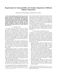
Abstract
Despite several decades of research, locomotion of bipedal robots is still far from achieving
the graceful motions and the dexterity observed in human walking. Most of today’s bipeds
are controlled by analytical approaches based on multibody dynamics, pre-calculated
joint trajectories, and Zero-Moment Point considerations to ensure stability. However,
beside their considerable achievements these methods show several drawbacks like strong
model dependency, high energetic and computational costs, and vulnerability to unknown
disturbances. In contrast to this, human locomotion is elegant, highly robust, fast, and
energy efficient. These facts gave rise to the main hypothesis of this thesis, namely that a
control system based on insights into human motion control can yield human-like walking
capabilities in two-legged robots.
This thesis thus presents a control methodology for bipeds relying heavily on the transfer
of concepts found in the locomotion control of humans. Based on a thorough review on
biomechanics and neuroscience literature, a control approach is derived that can achieve
dynamic, efficient, and robust walking of three-dimensional and fully articulated bipeds.
Being located above the neural level, the control system is structured as a hierarchical
network of local feed-forward and feedback units, without using a complete dynamic model
or pre-calculated joint trajectories. Sensor event-based spinal pattern generators coordinate
the stimulation and synchronization of control units and the compliance of passive joints.
By applying local torque commands instead of joint angle control, passive dynamics and
self-stabilizing effects of elasticities can be exploited. Postural control is achieved by the
phase-dependent activity of several reflexes of various complexity.
The suggested approach is tested in a full-featured dynamics simulation framework on an
anthropomorphic biped with 21 degrees of freedom and human-like morphology, weight,
and actuation. The control system can achieve three-dimensional dynamic walking of
variable velocity as well as balanced standing. It is able to cope with the high complexity
and the mechanical elasticities of the modeled biped. The emerging, naturally looking
walking gait shows remarkable similarities to human walking. Simultaneous control of
only a subset of joints is sufficient to direct the passive dynamics of the robot towards a
walking gait. The achieved walking velocity of up to 5 km/h can compete with even the
most advanced of today’s bipeds. At the same time, energy efficiency is much better than
in joint angle controlled robots. The control system shows considerable robustness against
unknown and unexpected disturbance like steps, slopes, or external forces.

Contents
1 Introduction 1
1.1 Objectives . . . . . . . . . . . . . . . . . . . . . . . . . . . . . . . . . . . . 3
1.2 Structure . . . . . . . . . . . . . . . . . . . . . . . . . . . . . . . . . . . . 5
2 Technical Control Methods for Bipedal Robots 7
2.1 Challenges in Bipedal Walking . . . . . . . . . . . . . . . . . . . . . . . . . 7
2.1.1 Dynamically vs. Statically Stable Walking . . . . . . . . . . . . . . 7
2.2 Common Methods in Controlling Bipeds . . . . . . . . . . . . . . . . . . . 10
2.2.1 Zero-Moment Point . . . . . . . . . . . . . . . . . . . . . . . . . . . 10
2.2.2 Virtual Model Control . . . . . . . . . . . . . . . . . . . . . . . . . 12
2.3 Examples for Technically Controlled Bipeds . . . . . . . . . . . . . . . . . 13
2.4 Assessment of Technical Control Approaches . . . . . . . . . . . . . . . . . 20
3 Human Locomotion Control 23
3.1 Structural Organization of Motion Control . . . . . . . . . . . . . . . . . . 23
3.1.1 Functional Morphology . . . . . . . . . . . . . . . . . . . . . . . . . 23
3.1.2 Neurological Basics . . . . . . . . . . . . . . . . . . . . . . . . . . . 26
3.1.3 Sensorimotor Interaction . . . . . . . . . . . . . . . . . . . . . . . . 30
3.1.4 Hierarchical Layout of Motion Control . . . . . . . . . . . . . . . . 32
3.2 Normal Walking in Humans . . . . . . . . . . . . . . . . . . . . . . . . . . 36
3.2.1 Biomechanical Gait Analysis . . . . . . . . . . . . . . . . . . . . . . 36
3.2.2 Phases of Walking . . . . . . . . . . . . . . . . . . . . . . . . . . . 47
3.2.3 Reflex Function during Walking . . . . . . . . . . . . . . . . . . . . 48
3.2.4 Postural Control . . . . . . . . . . . . . . . . . . . . . . . . . . . . 50
3.3 Key Aspects of Biological Walking Control . . . . . . . . . . . . . . . . . . 53
3.4 Biologically Inspired Control of Bipedal Robots . . . . . . . . . . . . . . . 55
3.4.1 Exploitation of Inherent Dynamics and Elasticities . . . . . . . . . 55
3.4.2 Neuro-, Reflex-, and Oscillator-based Control . . . . . . . . . . . . 60
4 A Biologically Supported Concept for Controlling Bipeds 67
4.1 Passive Control Aspects . . . . . . . . . . . . . . . . . . . . . . . . . . . . 67
4.2 Control Unit Classes . . . . . . . . . . . . . . . . . . . . . . . . . . . . . . 69
4.2.1 Locomotion Modes . . . . . . . . . . . . . . . . . . . . . . . . . . . 69
4.2.2 Spinal Pattern Generators . . . . . . . . . . . . . . . . . . . . . . . 70
4.2.3 Motion Phases . . . . . . . . . . . . . . . . . . . . . . . . . . . . . 70
4.2.4 Motor Patterns . . . . . . . . . . . . . . . . . . . . . . . . . . . . . 70
4.2.5 Local Reflexes . . . . . . . . . . . . . . . . . . . . . . . . . . . . . . 71
4.2.6 Postural Reflexes . . . . . . . . . . . . . . . . . . . . . . . . . . . . 71
4.3 Hierarchical Layout . . . . . . . . . . . . . . . . . . . . . . . . . . . . . . . 72

vi Contents
5 Controlling Dynamic Locomotion of a Fully Articulated Biped 75
5.1 System Premises . . . . . . . . . . . . . . . . . . . . . . . . . . . . . . . . 75
5.1.1 Kinematic Layout . . . . . . . . . . . . . . . . . . . . . . . . . . . . 75
5.1.2 Assumed Actuation and Sensor System . . . . . . . . . . . . . . . . 77
5.1.3 The Behavior-based Control Architecture iB2C . . . . . . . . . . . 77
5.2 Guidelines for Designing Control Units . . . . . . . . . . . . . . . . . . . . 81
5.2.1 Feed-Forward Control Units . . . . . . . . . . . . . . . . . . . . . . 81
5.2.2 Feedback Control Units . . . . . . . . . . . . . . . . . . . . . . . . 82
5.2.3 Guidelines for Implementing iB2C Features . . . . . . . . . . . . . . 83
5.3 Stable Standing . . . . . . . . . . . . . . . . . . . . . . . . . . . . . . . . . 83
5.3.1 Balanced Standing Control in Humans . . . . . . . . . . . . . . . . 83
5.3.2 Stabilized Standing Control . . . . . . . . . . . . . . . . . . . . . . 85
5.3.3 Stable Standing State Machine . . . . . . . . . . . . . . . . . . . . 85
5.3.4 Ground Adaptation . . . . . . . . . . . . . . . . . . . . . . . . . . . 86
5.3.5 Posture Stabilization . . . . . . . . . . . . . . . . . . . . . . . . . . 88
5.3.6 Posture Optimization . . . . . . . . . . . . . . . . . . . . . . . . . . 88
5.3.7 Relaxed Stance . . . . . . . . . . . . . . . . . . . . . . . . . . . . . 89
5.4 Dynamic Walking . . . . . . . . . . . . . . . . . . . . . . . . . . . . . . . . 90
5.4.1 Interrelation between Locomotion Modes . . . . . . . . . . . . . . . 90
5.4.2 Walking Initiation . . . . . . . . . . . . . . . . . . . . . . . . . . . 91
5.4.3 Spinal Pattern Generator for Walking . . . . . . . . . . . . . . . . . 95
5.4.4 Walking Phase 1: Weight Acceptance . . . . . . . . . . . . . . . . . 97
5.4.5 Walking Phase 2: Propulsion . . . . . . . . . . . . . . . . . . . . . 99
5.4.6 Walking Phase 3: Stabilization . . . . . . . . . . . . . . . . . . . . 101
5.4.7 Walking Phase 4: Leg Swing . . . . . . . . . . . . . . . . . . . . . . 102
5.4.8 Walking Phase 5: Heel Strike . . . . . . . . . . . . . . . . . . . . . 104
5.4.9 Posture Control . . . . . . . . . . . . . . . . . . . . . . . . . . . . . 105
6 Implementation of Bipedal Walking Control 113
6.1 Simulation Environment . . . . . . . . . . . . . . . . . . . . . . . . . . . . 113
6.1.1 Embedding the Physics Engine . . . . . . . . . . . . . . . . . . . . 113
6.1.2 Actuators and Joint Control . . . . . . . . . . . . . . . . . . . . . . 115
6.1.3 Simulation of Sensors . . . . . . . . . . . . . . . . . . . . . . . . . . 118
6.1.4 Model of Simulated Biped . . . . . . . . . . . . . . . . . . . . . . . 119
6.2 Notes on the Implementation . . . . . . . . . . . . . . . . . . . . . . . . . 121
6.2.1 Group Layout and Phase Representatives . . . . . . . . . . . . . . . 121
6.2.2 Application of iB2C Features . . . . . . . . . . . . . . . . . . . . . 122
7 Balanced Standing Experiments 125
7.1 Adaptation to the Ground Geometry . . . . . . . . . . . . . . . . . . . . . 125
7.2 External Forces and Platform Movements . . . . . . . . . . . . . . . . . . . 126
7.3 Posture Optimization . . . . . . . . . . . . . . . . . . . . . . . . . . . . . . 133

Contents vii
8 Dynamic Walking Experiments 137
8.1 Normal Walking . . . . . . . . . . . . . . . . . . . . . . . . . . . . . . . . . 137
8.1.1 Locomotion Modes . . . . . . . . . . . . . . . . . . . . . . . . . . . 137
8.1.2 Switching Walking Phases . . . . . . . . . . . . . . . . . . . . . . . 139
8.1.3 Behavioral Activity . . . . . . . . . . . . . . . . . . . . . . . . . . . 142
8.1.4 Kinematic Analysis . . . . . . . . . . . . . . . . . . . . . . . . . . . 148
8.1.5 Kinetic Analysis . . . . . . . . . . . . . . . . . . . . . . . . . . . . . 158
8.2 Walking under Disturbances . . . . . . . . . . . . . . . . . . . . . . . . . . 168
8.2.1 Sloped Terrain . . . . . . . . . . . . . . . . . . . . . . . . . . . . . 169
8.2.2 Walking over Steps . . . . . . . . . . . . . . . . . . . . . . . . . . . 174
8.2.3 Constant External Forces . . . . . . . . . . . . . . . . . . . . . . . 175
9 Conclusion and Outlook 177
9.1 Summary . . . . . . . . . . . . . . . . . . . . . . . . . . . . . . . . . . . . 178
9.2 Future Work . . . . . . . . . . . . . . . . . . . . . . . . . . . . . . . . . . . 182
A Biomechanical and Anatomical Terms 185
B Dynamics Simulation Framework 191
B.1 MCA2 and SimVis3D . . . . . . . . . . . . . . . . . . . . . . . . . . . . . . 191
B.2 Embedding of the Physics Engine . . . . . . . . . . . . . . . . . . . . . . . 193
B.3 Interface to Control System and Simulation . . . . . . . . . . . . . . . . . 195
B.4 Simulation Scenario for Biped Experiments . . . . . . . . . . . . . . . . . . 198
Bibliography 203

viii Contents

1. Introduction
Since many centuries, man is dreaming of creating an artificial servant as assistant in
daily life or as laborer for exhausting work. Before the advent of industrial robotics,
these moving machines built of inanimate matter have been imagined as likenesses of
man, working in humanly environment. The golem described in the Jewish folklore can
be seen as an early example, a figure of human shape being formed from clay. The tale
of Rabbi Judah Loew ben Bezalel tells of his creation of a golem to defend the Jewish
ghetto of the 16th century Prague against anti-Semitic attacks. Figure 1.1 shows Paul
Wegener’s interpretation of a golem in his silent movie series from 1920. The character
of the golem inspired many writers, like Johann Wolfgang von Goethe in his poem“The
Sorcerer’s Apprentice”, Mary Shelley and her novel“Frankenstein”, or the Czech writer
Karel ˘ Capek. His science fiction play“R.U.R.”(Rossum’s Universal Robots) from 1921
introduced clone-like artificial creatures working for and then rebelling against their human
creators. These androids are called Robots based on the Czech work robota meaning labor,
thus making the term known and popular.
While the golems, ˘ Capek’s robots, or Frankenstein’s creature are made of animated clay
or human tissue, the idea of an artificial laborer also infected inventors and engineers. As
early as 1886 Zadock Dederick built and was granted a patent for his Steam Man, a 250kg
heavy machine powered by a steam engine and pulling a rockaway carriage (Figure 1.1).
In 1893, George Moore adopted the idea and built a similar mechanical man, supported
by a horizontal bar and able to walk in circles. At the New York World’s Fair in 1939, the
robot Elektro was exhibited (Figure 1.1). Build by J.M. Barnett of the Pittsburgh-based
Westinghouse Electric Corporation as an elaborate marketing tool, the 120kg machine of
about 2.1m in height could move its mouth, fingers, and limbs. Triggered by simple voice
commands, it would replay recorded speech samples, walk, or smoke cigarettes. Similar
projects of that time include the radio controlled robot George by Pilot Officer Sale (1950),
Garco by Harvey Chapman (1953), Gygan by Piero Fiorito (1957), or MM47 by Claus
Scholz (1961).
The walking mechanisms of the machines mentioned above were of rather primitive form,
the leg movement mostly induced by a single rotating motor and straight-line linkages. To
enable more robust locomotion on uneven ground, more sophisticated constructions became

2 1. Introduction
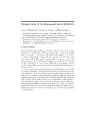
Figure 1.1: The Golem in Paul Wegener’s silent movies (1920), Steam Man created by Zadock
Dederick (1886), Elektro built by the Pittsburgh-based Westinghouse Electric Corporation (1938),
WL-1 (1967) and WABOT-1 (1973), developed by Ichiro Kato, Waseda University.
necessary. The development of walking machines aroused the interest of the scientific
community. Ichiro Kato of the Waseda University in Japan started his pioneer work on
bipedal robots in 1966. His first robot WL-1 from 1967 is shown in Figure 1.1, WL-3
developed in 1969 could already perform preliminary static walking as well as standing
and sitting motions [Lim 06]. In 1973, Kato’s group built the robot WABOT-1, which is
commonly accepted as the first fully articulated anthropomorphic biped [Kato 73].
With the emergence of complex machines like those developed by Kato and others, and
the availability of microprocessors, it soon became apparent that not only the mechanical
design but also the control of bipedal robots poses challenging problems. While Rabbi
Loew could simply write the instructions for his golem on a piece of paper and place it
in the golem’s mouth, controlling two-legged locomotion turned out to be much more
difficult. The high center of mass, the small support area spanned by only two feet,
and an essentially dynamic gait make preserving balance and stability a tough job. As
robotics scientists mainly emerged from mechanical engineering, the mathematical tools
and concepts of this research field where applied to find fitting control strategies, the
most prominent one being Vukobratović’s Zero-Moment Point concept. It found its first
application in 1984 on Kato’s robot WL-10RD and will be described in detail later in
this thesis. Since then, the majority of research projects on bipedal robots complied with
these ideas and methods. Mainly located in Japan and other Asian countries, these efforts
yielded impressive machines like Honda’s Asimo or Kaist’s Hubo.
But in spite of over four decades of research, the problem of mechanical bipedal locomotion
is still far from being solved. Compared to the elegant and efficient walking motions of
humans, even the most sophisticated bipedal robots appear clumsy and slow. One possible
way of improving the performance of two-legged walking machines could be the transfer of
ideas from biology, not only in respect to the mechanical setup, but also to the control
concepts.
The knowledge necessary for this approach can be found in research on biomechanics
and neurosciences. As with the urge for an artificial servant, man’s aspiration to know
the working of his own body has a history of many centuries. Aristotle (384–322 BC) is
commonly seen as founder of kinesiology, the science of movement of the body. In his book

1.1. Objectives 3
“De Motu Animalium”he was the first to treat the action of muscles and their geometrical
relationship to extremities, and to analyze walking as cyclic motion. The studies of
Archimedes (287–212 BC) on gravity and leverage laid the foundation to mechanical
analysis of motion. The Roman physician Galen (AD 131–201) introduced the principle
of antagonistic muscle work or the distinction between muscle and sensory nerves in his
treatise“De Motu Musculorum”, considered to be the first textbook on biomechanics.
It was up to Leonardo da Vinci (1452–1519) to further the field of kinesiology during the
Renaissance after many centuries of stagnation. The artist and scientist had an interest in
the structure of the human body and tried to identify muscles, nerves, and the mechanics
of the body during various motions. In 1543, the Flemish physician Andreas Vesalius
published his text“On the Structure of the Human Body”, correcting some of the error
made by Galen. In the late 16th and the following century, important contributions can
be attributed to Galileo Galilee, Marcello Malpighi, and especially to Giovanni Alfonso
Borelli. He was the first to understand that the forces produced by muscles have to be
larger than those acting against the skeletal motion, as the levers of the musculoskeletal
system magnify motion rather than force. This was even before Isaac Newton (1642–1727)
wrote his famous work“Principia Mathematica Philosophiae Naturalis”containing the
three laws of rest and movement, being essential for the analysis of body dynamics. In
the 18th century, electricity replaced the notion of“animal spirits”as origin of muscle
activation. Luigi Galvani (1737–1798) first stated the presents of electrical potentials in
muscles and nerves. In 1748 David Hartley established the term reflex as an automatic
response to a stimulus.
The 19th century saw the beginning of modern gait analysis. The Weber brothers
published their book “Die Mechanik der Menschlichen Gehwerkzeuge”, describing the
natural frequency of a pendulum-like leg swing and establishing the mechanism of muscular
action on a scientific basis. The arise of photographic techniques applied by Eadweard
Muybridge or Jules Marey allowed more detailed analysis of motion. Christian Wilhelm
Braune and Otto Fischer experimentally determined the body’s center of gravity. Adolf
Eugen Fick (1829–1901) introduced the terms isometric and isotonic during his analysis of
the mechanics of muscular movement and energetics. Sherrington’s work“The Integrative
Action of the Nervous System”is published in 1906. Sixteen years later, Archibald V.
Hill (1886–1977) receives the Nobel Prize for his studies on the oxygen consumption
during muscle work. In the middle of the 20th century, analyzing dynamic motions and
scrutinizing the“why”of human movement began to dominate research on biomechanics
and neurosciences. This objective has not changed up to now, and still human motion
control is far from being completely understood. Nevertheless, recent results in these fields
encourage the transfer of biological concepts to the design and control of technical systems.
Combined with the advances made in the development and control of complex robotic
systems, this strategy acted as motivation for the work at hand.
1.1 Objectives
The goal of this thesis is the derivation of a control methodology for dynamical locomotion
of bipedal robots based on concepts found in human motion control.
This goal is based on the hypothesis that a control system similar to the human one will
enable a robot to perform locomotion in a likewise fashion. Obviously, neither all aspects

4 1. Introduction
of human motion control nor all capabilities of human locomotion can be expected to be
considered or included. A reasonable subset needs to be regarded that is tailored to be
applicable to bipedal robots with today’s technical means, but still is as general as possible
to allow a broad range of motions and skills. Balanced standing and three-dimensional
dynamic walking of a fully articulated anthropomorphic biped shall be the target forms of
locomotion for this work. This allows to analyze the control performance during both more
static and dynamic motions of a complex robotic system. Further modes of movement like
running or jumping should potentially be viable.
While the results of a single thesis surely cannot fully compete with the abilities of machines
developed over decades, it at least should be shown that some of their drawbacks can be
overcome. As in the natural example, a walking style of less clumsiness, higher speed, or
better efficiency should be expected. In case a comparison to human walking should result
in substantial similarities, e.g. regarding joint angle trajectories, even a step towards the
confirmation of biomechanical or neuroscientific hypotheses could be ventured.
To design a biologically inspired control concept in correspondence to the goal just
formulated several issues have to be addressed. The following topics are regarded as being
crucial and thus will be approached in detail within this thesis:
Analysis of Recent Results from Biomechanics and Neuroscience
As mentioned on the previous pages, biomechanics and neuroscience have a long lasting
history. Accordingly the state-of-the-art on these topics is extensive and still growing.
Nevertheless it needs to be examined to identify the key aspects of human motion control
that have the potential to be transferred to a robotic control system. Fortunately, some
researchers of these disciplines have already offered some advice for the robotics community
that can serve as starting point for the analysis.
Dependence of Mechanics and Control in Human Motion Generation
It can be assumed that during the course of evolution, the human morphology has been
optimized towards bipedalism. Research on functional morphology can help to identify
the properties of the musculoskeletal system essential for locomotion. While this work’s
objectives cannot include the development of mechanical solutions, still properties like
muscle characteristics, mass distribution, or limb geometry need to be analyzed as control
aspects are depending on them. Especially potential exploitation of passive dynamics
should be considered.
Granularity and Classes of Suitable Control Units
The selected biological key aspects have to be transferred to a technically feasible control
approach. As this thesis follows the concept of behavior-based robot control, a suitable
fusion of conceptual ideas needs to be found. This implies that the granularity of control
units should be above the level of biological neurons. A set of classes of such control units
should be derived from the functional units found in natural motion control, including
feedback as well as feed-forward mechanisms. To arrange such control units and to manage
their communication, a structural layout needs to be defined serving as a design guideline.

1.2. Structure 5
Implementation of Dynamic Walking within the Control Concept
Having determined relevant classes and a control structure, the control units necessary
to synthesize dynamic walking need to be designed. Functional units identified in the
analysis of human walking have to be mapped to the suggested control concept. Solutions
for the implementation of the derived control units must be developed. As a bipedal robot
will never be an exact copy of the human morphology, adaptation of these units as well as
the design of new units will be necessary.
Test Environment for Validation
Lacking an actual robot featuring the properties relevant for human-like dynamic walking,
a suitable model needs to be developed within a simulation environment. The simulation
has to reflect physical effects like gravity, mass distribution, or collision, otherwise dynamic
locomotion and exploitation of passive dynamics could not be observed.
Naturally, there already has been and still is research on the transfer of control aspects from
biology to walking machines, as will be presented in Chapters 3. Hence this thesis aims at
differing from previous work regarding the extend of including biological analysis and the
resulting applicable control aspects, the manner in which these aspects are transformed
into a robot control system, and the complexity of the considered robotic target platform.
Only a small minority of the research projects on biologically motivated robot control has
been applied to the dynamic walking of a fully articulated biped. Finally, as this work
introduces behavior-based control concepts to bipedal robot control, it can be examined if
this harmonizes with the biologically motivated approach or can bring additional benefits
compared to other control methods.
1.2 Structure
This thesis is structured as follows:
Chapter 2 begins by defining the main challenges of dynamic bipedal walking that have to
be handled by the control system. Then common control methods like the Zero-Moment
Point approach are introduced. These methods are based on techniques from mechanical
engineering or industrial robotics, e.g. multibody dynamics, and will be called technical
control methods in contract to biologically inspired ones for the remainder of this work.
The state-of-the-art of these approaches is reviewed and their advantages and drawbacks
are assessed.
In order to develop a human-like biped control system, Chapter 3 introduces basic and
advanced aspects of human locomotion control, both regarding its structural organization
and its functional analysis. Based on these results from biomechanical and neuroscientific
research, key aspects of biological walking control and implications for robotics are derived.
The chapter concludes with an evaluation of literature on biologically inspired control of
two-legged robot locomotion.
In Chapter 4, the insights just gained are used to design a control concept for dynamic
bipedal locomotion. It is discussed how passive dynamics can be exploited and in what
way they influence the control system. Classes of control units are suggested based on
active feed-forward and feedback mechanisms observed in human walking. These control

6 1. Introduction
units are arranged in a hierarchical layout similar to the structure that is assumed to exist
in biological locomotion control.
Chapter 5 describes the design and implementation of stable standing and dynamic
walking control applying the suggested methodology. First, requirements regarding the
mechatronics and the control system of the target platform are given. Then it is discussed
how suitable control units can be found, e.g. by consulting gait analysis research. Next,
the control units and the resulting network for balanced standing on uneven surfaces and
under external disturbances as well as for dynamic walking are introduced.
The simulation environment and the model of the bipedal robot used for the experiments
are presented in Chapter 6. Additionally, it contains notes on particularities of the
implementation regarding the behavior-based architecture and the control framework.
The experiments on stable standing are described in Chapter 7. It is shown how the robot
adapts to the ground geometry and how it reacts to external disturbances. Furthermore,
the results of the posture optimization method are presented.
Finally, Chapter 8 analyzes the performance of the suggested control system during
dynamic walking. Behavioral activity as well as kinematic and kinetic progresses are
discussed. The resulting motions are compared to data from human gait analysis. The
robustness of the control system is evaluated by applying different disturbances during
walking.
The thesis is concluded in Chapter 9. The main aspects and contributions of the suggested
control methodology are summarized and an outlook on possible future research is given.
A short glossary on biomechanical terms, some anatomical guidance, and details on the
implementation of the simulation framework are given in the appendices.

2. Technical Control Methods for
Bipedal Robots
Looking at control methods for two-legged robots two fundamentally different approaches
can be observed: the technical and the biological approach. In this thesis technical control
approaches are understood as the class of methods mainly based on insights from industrial
robotics and mechanical engineering. They draw on sound mathematical concepts like
multibody dynamics, linear and nonlinear control theory, or established joint constructions
and materials from industrial robots. Biologically inspired approaches try to transfer
results from human motion analysis, biomechanics, or neuroscientific research to technical
system. While not totally dismissing approved mathematical and engineer’s resources,
they focus more on new materials and actuation systems, intelligent mechanics, and, most
notably, on adopting control concepts found in nature.
This chapter will review the technical control approaches as they are most commonly used
for bipeds. Then it will be argued that it is well worth looking at how nature is creating
and controlling bipedal locomotion, as done in the subsequent chapter. But to start with,
the main challenges in controlling two-legged locomotion will be introduced. These apply
to the technical as well as the biological control methods.
2.1 Challenges in Bipedal Walking
The task of getting a bipedal robot to walk can be divided into several separate problems.
For each of these challenges a solution must be found to achieve stable, cyclic locomotion.
This section will shortly introduce this set of problems to enhance the understanding on
the subject matter of this thesis. However, first there must be distinguished between two
fundamentally different ways of walking.
2.1.1 Dynamically vs. Statically Stable Walking
Walking can be performed in two entirely different ways: statically or dynamically stable.
This holds true not only for two-legged walking, but also for other multipeds like four-legged

8 2. Technical Control Methods for Bipedal Robots
support
CoM
support
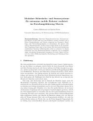
Figure 2.1: Statically stable walking keeps the projection of the center of mass inside the
support area, dynamic walking allows for temporarily instability.
mammals. In statically stable walking it is possible to freeze the motion at any time
without risking instability. This can only be achieved by always keeping the projection of
the center of mass within the support area of the feet with ground contact. For bipedal
walking this creates the necessity to first fully move the weight of the body over the foot
of the next stance leg before the swing foot can leave the ground. As a result statically
stable walking, while guaranteeing stability, is comparatively slow and tedious, consumes
more energy, and limits the possible step length.
In contrast, dynamically stable walking, or dynamic walking in short, does not pose
limitations that hard on the trajectory of the center of mass. Rather, it must be ensured
thatinstabilityremainstemporarily. Toputitsimply, dynamicwalkingmeanstoconstantly
fall, but to bring forward the swing leg in time to prevent tilting over. This far more
efficient kind of walking allows for higher velocity by larger step size, shorter double
support phase, and less time consuming adjustment of weight distribution. Figure 2.1
illustrates the difference by showing projection of the center of mass during a statically
and dynamically stable step.
Nearly all walking found in two- or four-legged vertebrates is dynamic. If at all, statically
stable walking can be observed in very slow or cautious locomotion, or in case highly
deliberate foot placement is necessary. In bipedal robots, both ways of walking can and
have been realized with dynamic walking being the considerably more challenging control
problem. Possible approaches to achieve this behavior will be discussed later in this chapter
and at the end of the next one.
As this thesis focuses on dynamic walking, from now on this way of locomotion is implied,
and the distinction is explicitly made when talking about the statically stable case. The
challenges of walking described in the following also deal with dynamic locomotion, even if
several of these problems must also be tackled for the statically stable alternative.
Transition between Stance and Swing
Walking is a process of discrete phases and transitions: each leg switches its role from
stance to swing, and the biped alternates between single and double support. The challenge
here is to find the proper point in time when to switch from double to single support and
CoM

2.1. Challenges in Bipedal Walking 9
Figure 2.2: A typical step during normal dynamic walking of a human subject from one heel
strike to the next.
back again. If the rear leg is lifted too early, energy to transfer the body over the stance
leg might be insufficient. Lifted too late, the time to swing the leg forward to support
the body will be too short. Also, the objectives of the control units involved may change
depending on the walking phase. Switching from one phase to the next can be triggered by
sensory events or after a certain amount of time. Figure 2.2 illustrates the phases during
normal dynamic walking by showing a typical step of a human subject from one heel strike
to the next. The swing phase lasts for about one third of the whole stride’s time. The key
events normally referenced in bipedal robotics as well as in biomechanical gait analysis are
foot strike, midsupport, toe-off, forward swing, and deceleration.
Support of the Trunk
During its stance phase, a leg must support the weight of the upper body. The trunk
height is a result of the stance leg’s length, which can be kept straight or act as virtual
spring. If the leg is kept stiff, more potential energy must be used to lift the upper body
as it moves forward like an inverted pendulum, but the torque in the knee can remain low.
In case the knee is bended, the leg length must be synchronized with the translation of
the trunk.
Leg Swing
The forward swing of the leg has to meet two conditions: the foot must clear the ground,
and the leg must arrive in front of the body in time to act as next swing leg. Ground
clearance can be achieved through shortening the leg by bending the knee, and by keeping
the foot oriented level to the ground. Uneven terrain can make this task even more difficult.
The swing duration can be shortened by accelerating in the hip joint, but the maximum
hip torque confines the minimal duration and as such the maximum walking velocity given
a maximum step length.
Control of Forward Velocity
The appropriate forward velocity of the upper body is crucial for stable dynamic walking.
As the system acts like an inverted pendulum while traversing over the stance leg, enough
kinetic energy must be present to be transferred to potential energy of the upper body.
In contrast, if the velocity is too high, the time for the swing leg to travel before the
body might be too short and the biped tumbles. During walking, energy is consumed by
damping and by foot impact. Measuring or estimating the proper forward velocity is not
easily achieved.

10 2. Technical Control Methods for Bipedal Robots
The forward velocity can be influenced by many factors: the further back the center of
pressure is located in the stance foot during single support, the faster is the resulting
forward movement. Bending the trunk forward accelerates the biped, leaning backwards
slows it down. During double support, the center of mass can be transferred forward
or backwards within certain limitations. A push-off motion using the ankle of the rear
leg before lifting it inserts energy into the system, too. Finally, the timing of the phase
transition events as well as the variation of the step length change the amount of time the
body mass is in front of and behind the stance leg, and thus is accelerating or decelerating
the robot.
Stability of the Trunk in the Sagittal Plane
Keeping the upper body erect or purposefully leaning it forward or backwards as just
mentioned is a further objective during walking. Trunk pitch is disturbed by inertia during
foot impact as well as by gravity as its center of mass lies above the hip joint. It is further
influenced by hip torques generated during leg swing.
Lateral Stability
While the challenges mentioned so far also hold true for planar walking, i.e. walking
confined to the sagittal plane, lateral movement is only introduced in three-dimensional
locomotion. Foot impact can heavily disturb lateral stability. Keeping the biped from
falling to one side can be reached by leaning the upper body sidewards, by applying
torque in the ankle joints, or by shifting the foot position of the swing leg to the left or
right. While the first two methods only allow marginal influence, the last one can even
compensate strong sidewards motions, however it must potentially act over several strides.
Introducing feedback control for both lateral and anterior/posterior stability requires an
estimation of the upper body’s orientation. Given an unknown ground orientation, this
cannot be calculated by kinematics. Sensor systems like inertial measurement units or
vision systems gauging the horizon can provide the necessary information.
2.2 Common Methods in Controlling Bipeds
Nature was not the first choice when biped engineers first looked for inspiration on how
to control two-legged walking machines. Rather, established methods from electrical and
mechanical engineering like multibody dynamics or classical control theory served as basis
for the development of control systems. This section will review the most prominent and
more recent developments of biped research to illustrate the technical control approach.
Most of the control systems for walking bipedal robots are based on Vukobratović’s Zero-
Moment Point (zmp) approach [Vukobratovic 72, Vukobratovic 04] or the derived Center
of Pressure (cop) approach [Sardain 04]. Regarding the prominent role of the zmp, the
next section will give a short overview on its ideas.
2.2.1 Zero-Moment Point
The zmp describes a criterion for dynamic balance first formulated by Miomir Vukobratović
in 1968. It is defined as that point on the ground at which the net moment of the inertial
forces and the gravity forces has no component along the horizontal axes.

2.2. Common Methods in Controlling Bipeds 11
Figure 2.3: Visualization of the Zero-Moment Point. From [Vukobratovic 04], p160.
Let us consider a biped robot in single support phase. The influence of the dynamics of the
segments above the ankle is represented by the force FA and the moment MA (Figure 2.3b).
The ground reaction in point P consists of the force R = (RX,RY,RZ) and the moment
M = (MX,MY,MZ). The friction of the non-sliding foot on the ground compensates the
horizontal components of FA and the vertical part of MA (Figure 2.3c) and can therefore
be represented by (RX,RY,MZ). RZ represents the ground reaction that balances vertical
forces. The remaining horizontal components of active moments can only be compensated
by shifting the position P of the reaction force R within the support polygon (Figure 2.3d).
If the support polygon of the foot is not large enough for an appropriate position of R, the
force acts at the edge of foot and a uncompensated component of the reaction moment
remains. This results in a rotation about the foot edge and the robot stumbles. Therefore
the condition for the robot to be in dynamic equilibrium can be given for the point P on
the foot sole where the ground reaction force is acting:
MX = 0 and MY = 0 (2.1)
The point P is then called the Zero-Moment Point. The static equilibrium equations for
the supporting foot can be given as
R+FA +msg = 0, (2.2)
−→
OP ×R+ −→
OG×msg +MA +MZ + −→
OA×FA = 0, (2.3)
where O is the origin of the coordinate system, P the ground reaction force acting point,
G the foot’s center of mass, A the ankle joint, and ms the foot mass.
Projecting Equation 2.3 onto the horizontal plane gives
( −→
OP ×R) H
+ −→
OG×msg +M H A +MZ +( −→
OA×FA) H
= 0 (2.4)
which is the basis for computing the ground reaction force acting point P. To ensure
dynamic equilibrium, the point P must be within the support polygon. If the computed

12 2. Technical Control Methods for Bipedal Robots
Figure 2.4: The ground reaction force acting point P must be within the support polygon.
From [Vukobratovic 04], p164.
point is outside the support polygon (called fictitious, fzmp then), the zmp does not exist
as Equation 2.1 is not met and the ground reaction force acting point P is actually on
edge of support polygon. This results in a rotation around the foot edge and the loss of
balance (Figure 2.4).
The zmp can be used for the task of offline gait synthesis or as a key indicator for online
gait control. It can be measured approximately by force sensors in the foot sole of the robot.
An extension to the zmp and cop can be found in the foot-rotation-indicator [Goswami 99].
It is identical to the cop when located within the foot’s support area, but when outside
it gives information about the degree and direction of postural instability. Most of the
bipeds presented in the following are using zmp calculation as part of their control system.
2.2.2 Virtual Model Control
Another methodology for the control of bipedal robots is the Virtual Model Control
developed by Jerry Pratt [Pratt 95b, Pratt 01]. The goal of this approach is to keep the
control algorithms easy to understand and intuitive.
The idea of Virtual Model Control is to apply forces to the robot via virtual components
that are attached within the robot or between the robot and the environment. The
resulting actual joint torques and forces create the same effect that the force of the virtual
component would create. These components, which have to create a force based on their
state, might include springs, dampers, masses, potential field, or others. The placement of
the components remains with the designer and requires physical intuition. No complete
dynamic model of the robot is required. The equation describing the static dynamics for a
serial link chain is given as
τ = J T F (2.5)
where τ are the joint torques, J is the Jacobian relating the two attached frames of the
virtual components, and F is the force produced by it.
Robots controlled by Virtual Model Control include a simulated six legged walking
machine [Torres 96]. The 18 degree of freedom robot can walk in any direction, turn, and
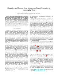
balance an inverted pendulum on its back. The bipedal robot Spring Turkey (Figure 2.5a)
can walk in the sagittal plane [Pratt 97]. Each leg has an active degree of freedom in its
knee and hip, but not feet or ankle. The robot is supported and balanced by a virtual
“granny walker”composed of two springs and dampers (Figure 2.5b). Control of forward
speed during double support is realized by a virtual“dog-track bunny”connected to the

2.3. Examples for Technically Controlled Bipeds 13
(a) (b)
Figure 2.5: (a) The bipedal robot Spring Turkey. (b) Virtual components are attached to the
robot. From [Pratt 97], p197.
robot by a damper. The coordination of the legs is realized by a virtual“reciprocating gait
orthosis”. A state machine selects the components during the different phases of walking.
Spring Turkey can walk in a not so robust manner at a speed of up to 0.5m. The robot s
Spring Flamingo is also partly controlled by using the Virtual Model Control and discussed
in Section 3.4.1.
2.3 Examples for Technically Controlled Bipeds
Since four decades, reseach institutes throughout the world have been developing bipedal
robots. Despite their anthropomorphic appearance, most of the efforts follow a more industrial
approach in the design and control of their machines and apply the aforementioned
zmp calculation for generating joint trajectories. The most prominent representatives of
this kind of robots are described in the following section, two of them in more detail.
The H7 Robot by the JSK Laboratory
The Jouhou System Kougaku (jsk) Laboratory of the University of Tokyo has a long
tradition of building humanoid robots, some of which are shown in Figure 2.7. The aim
of its work is to develop an experimental research platform for walking, autonomous
behavior and human interaction. The design of their latest robot H7 focused on additional
degrees of freedom (resulting in 30), extra joint torques, high computing power, real-time
support, power autonomy, dynamic walking trajectory generation, full body motions,
and three-dimensional vision support. Being 1.5m tall and weighting 57kg, the robot
features 7 degrees of freedom per leg including an active toe joint. A real-time capable
on-board computer, four lead-acid batteries, wireless lan, two ieee1394 high resolution
cameras, 6-axis forces sensors and an inertial measurement unit complete the robot’s
equipment [Kuffner 01, Chestnutt 03, Nishiwaki 06].
The online walking control system of H7 allows to generate walking trajectories satisfying
a given robot translation and rotation as well as an arbitrary upper body posture. It
is composed of several hierarchical layers as shown in Figure 2.6. Each layer represents
a different control cycle and passes its processed results to the next, lower layer which
usually runs at a higher frequency.
The gait decision layer chooses the gait and calculates the footstep locations. The algorithm
proposed by the authors determines the next swing leg’s foot point relative to the foot

14 2. Technical Control Methods for Bipedal Robots
Figure 2.6: Hierarchical layers of the dynamic walking control system of the robot H7.
From [Nishiwaki 06], p83.
of the supporting leg. Given a desired torso motion per step of (x,y,θ) with x being the
forward, y the sideward and θ the rotational offset, the next foot point is set at (x,2y±w,θ)
from the support foot, with w being the normal foot distance. Furthermore, geometrical
collision conditions are considered.
Generating dynamically stable walking trajectories in the next layer is based on Zero-
Moment Point considerations. Rather than analytically deriving the zmp trajectory from
the robots motion, the authors suggest a method with the walking trajectories following a
given zmp trajectory by horizontally shifting the torso. The starting point is an initial
robot trajectory
A(t) = (...,xi(t),yi(t),zi(t),θi(t),...). (2.6)
describing the position and orientation for each of the robot’s segments. Given the gravity
g and the position (xi,yi,zi), the mass mi, the inertia tensor Ii, and the angular velocity
ωi of each robot link i, the x component (y similar) of the zmp P = (xp,yp,0) T can be
calculated as �
mizi¨xi −
xp =
� {mi(¨zi +g)xi +(0,1,0) T Ii, ˙ωi}
− � (2.7)
m1(¨zi +g)
resulting in a zmp trajectory PA(t) = (xpa(t),ypa(t),0) T for the robot trajectory A(t). A
(t),0) can be followed by finding horizontal and
desired zmp trajectory P∗ A (t) = (x∗pa (t),y∗ pa
vertical shifts x ′ i(t) and y ′ i(t) for each link of the robot. For this, the following equation
must hold true, where xe p = x∗ p −xpa,x e i = x ′ i −xi
x e p =
� mizi¨x e i − � mi(¨zi +g)x e i
− � m1(¨zi +g)
. (2.8)
If a uniform horizontal body shift is assumed, i.e. the whole upper body moves consistently
(x e i = x e ), equation 2.8 can be transformed to
x e p =
� mizi
− � m1(¨zi +g) +xe . (2.9)

2.3. Examples for Technically Controlled Bipeds 15
Figure 2.7: Humanoids developed by the jsk Lab of the University of Tokyo: H5, H6, and H7.
After discretizing time and assuming certain boundary conditions, xe (i) can be obtained
from equation 2.9 in trinomial form, resulting in a robot trajectory following the desired
zmp trajectory P∗ A (t). This method requires that mass, inertia and pose are known for all
robot links.
A walking trajectory is then calculated online for each footstep, but already for three
steps in advance. Although normally only the first of these steps is used, the next two
pre-calculated steps would bring the robot to a stop, thus improving the systems safety.
Furthermore it is checked for each generated trajectory whether it remains within joint
angle and velocity limits, and whether it is free of self-collision.
Inthelastlayerbeforethemotorservolayer, thegeneratedwalkingtrajectoriesaremodified
based on sensor feedback. This step aims at compensating disturbances, modelling errors or
changes in the environment. Three controllers are used to achieve this: the horizontal torso
position is shifted according to the difference between the desired and the measured zmp;
the roll deflection of the upper body is compensated based on the inertial measurements;
and the servo gain is lowered before foot contact to lower the impact of ground reaction
forces.
Higher levels of H7’s control system deal with foot point planing in environments containing
obstacles, with object manipulation, or with full-body motion planing. Furthermore,
autonomous behavior is improved using the visual system by object tracking or 3D
reconstruction of the environment.
The Humanoid Robotics Project (HRP) by AIST
The National Institute of Advanced Industrial Science and Technology (aist) in Tsukuba,
Japan and Kawada Industries are developing the HRP robots since 1998 supported by
the Humanoid Robotics Project of the Ministry of Economy, Trade and Industry (meti).
Figure 2.8 shows the latest models of this research project. The robot HRP-2 features 35
degrees of freedom and is able to walk, lay down and stand up again [Kaneko 04]. Again,
the locomotion control system is based on zmp calculation [Kaneko 02b, Kajita 03].
The approach used a simplified dynamic model of the robot to enable online reference zmp
trajectory calculation. Assuming an inverted pendulum constrained to a horizontal plane

16 2. Technical Control Methods for Bipedal Robots
Figure 2.8: The HRP robot series developed by the National Institute of Advanced Industrial
Science and Technology in Tsukuba and Kawada Industries: HRP-2LR, HRP-2P, HRP-2,
HRP-3P, and HRP-3
of height zc as replacement model of the robot moving in the x/y-plane, the dynamics of
the system can be described as (similar in y-direction)
¨x = g
zc
+ 1
τy, (2.10)
mzc
where g denotes gravity, x the position of the body, m its mass, and τy the torque about
the y-axis. This linear dynamics is called the Three-Dimensional Linear Inverted Pendulum
Mode (3d-lipm). From this relation the position of the zmp can be calculated as
px = − τy
. (2.11)
mg
When substituted in equation 2.10 and rewritten as needed for the control of the zmp
position , it results in
px = x− zc
¨x.
g
(2.12)
Assuming the robot’s center of mass (CoM) position is given as (x,y) in the equations
above, the resulting zmp can easily be calculated. But generating a walking pattern is the
inverse problem: given a reference zmp trajectory, the movement of the center of mass is to
be found. The authors propose to formulate the zmp control as a servo problem. Defining
the time derivative ux of the horizontal acceleration ¨x as output of a servo controller
working on the zmp error pref −p and as input of a reformulation of equation 2.12, the
system shown in Figure 2.9 can calculate the CoM trajectory.
But in this way the CoM is only moved as soon as the zmp reference value is shifted, but it
should start moving before this to achieve the desired zmp. Thus a control concept known
as“previewcontrol”isused, previouslydescribedbyKatayamaetal.in1985[Katayama 85].
By first discretizing equation 2.12, an optimal preview servo controller is designed resulting
inacontrollaw foru(k) containing anerrortermbasedonthezmp error, a state termbased
on the CoM position, and a preview term based on the future zmp reference trajectory.
Using a preview length of 1.6s, good matching of the zmp trajectory can be achieved.
If the multibody model of HRP-2P is used instead of the simplified one, tracking errors of
the reference zmp can be observed. In order to compensate this, the authors suggest using

2.3. Examples for Technically Controlled Bipeds 17
Figure 2.9: Generating a CoM trajectory by tracking the zmp. From [Kajita 03], p1622.
a second preview control using the tracking error from the multibody model as input. In
doing so, the maximum zmp error can be reduced sufficiently. Using walking patterns
generated by this approach, spiral stair climbing of the simulated HRP-2P could be shown.
Several further improvements to this walking algorithm have been proposed. By adding
an additional zmp control based on sensor feedback and virtual time shift of the reference
zmp trajectory, walking on uneven terrain can be achieved with the simulated HRP-
2 [Kajita 06]. Further enhancements to the gait can be reached by adding a passive toe
joint [Sellaouti 06]. Higher walking speed and longer steps are made possible by adding an
under-actuated phase during the single support phase before heel strike and by adapting
the reference zmp trajectory accordingly. Recently, additional skills like sitting on a chair
or opening and passing through a door have been shown [Arisumi 09, Escande 09].
Besides the fully articulated HRP robots, advanced leg modules without an upper body
have been developed to investigate more sophisticated ways of locomotion. Using these
robot (HRP-2L, HRP-2LR and HRP-2LT) running-like motion could be achieved using
inverted pendulum based control trajectories [Kaneko 02a, Nagasaki 03, Kajita 05]. The
elasticity necessary for running is simulated by an active control of the dc motors instead
of exploiting passive, mechanical elasticity. Adding a toe spring increases running speed up
to 3 km/h in simulation [Kajita 07]. Currently, a dust and water proof version of the HRP
robot series is being developed [Akachi 05, Kaneko 08]. It can keep a balanced posture
while handling tools like an electric screwdriver.
Further Technically Controlled Bipeds
TheWasedaUniversityisdevelopingbipedalrobotssince1966. Themostrecentinstallment
of their research is the Wabian-2R robot (WAseda BIped humANoid) featuring a total
of 41 degrees of freedom [Ogura 06a]. Based on Zero-Moment Point calculations, a more
human-like walking with stretched knees and toe-off motion could be achieved [Ogura 06b].
The pattern generation approach generates trajectories for the feet using inverse kinematics
and Newton-Euler dynamics calculation. The knee trajectory is predetermined using cubic
splines rather then exploiting the natural dynamics of the system. Compensatory motions
in the waist maintain the robot’s balance according to the zmp trajectory. An iterative,
genetic algorithm optimizes the calculated trajectories in order to minimize waist rolling,
hip joint pitching, and ankle pitching.
In 1984 the company Honda began to work on humanoid robots. The P2 robot was
introduced in 1996 and can statically walk in any direction as well as climb stairs. Its six
degree of freedom legs feature damping to reduce the impact on the joints while walking.
The control system uses a detailed model of the robot and its foreknown environment

18 2. Technical Control Methods for Bipedal Robots
Figure 2.10: Further technically controlled humanoids: Asimo, KHR-3 (HUBO), Johnnie, and
Wabian-2.
and calculates stable trajectories with the help of the zmp method [Hirai 98]. The newest
Honda robot called Asimo is equipped with 28 degrees of freedom at the height of a
child [Sakagami 02]. While recent research focuses on its cognition skills and interaction
with humans [Mutlu 06], the robot possesses an elaborate locomotion system. As the
zmp-based walking approach is already working rather solid, further work is done on e.g.
footstep planing [Chestnutt 05]. With a specialized model of Asimo, running motions of
up to 10 km/h can be achieved [Takenaka 09b].
TherobotJohnnie hasbeendevelopedattheUniversityofMunichstartinginthelate1990s
with the aim to achieve jogging motions [Gienger 00, Lohmeier 04]. It is equipped with 17
joints and a sophisticated sensor setup. Using acceleration and gyroscopic sensors, the
attitude of the trunk is calculated including acceleration compensation to balance the robot
throughout the walking cycle. Cartesian trajectories for the center of gravity, the rotation
of the upper body, and the foot pose are derived as fifth-order polynomials from reduced
dynamic models and zmp positions. The computed torque method used for the modeling
allows to consider the entire system dynamics for the control of the robot [Löffler 03].
This model-based control poses high demands on the computational performance, the
communication bandwidth, and the frequency of the sensor data. Therefore, the intended
running motion could not be achieved. This goal is hoped to be reached with the successor
Lola by reducing the weight, introducing new sensor systems, and revising the control
concept [Lohmeier 06, Buschmann 09].
Further robots of similar design and control approach are the KHR-2 and KHR-3 (aka.
HUBO) by Kaist in Korea [Kim 05, Park 05], BHR-2 of the Beijing University of Science
and Engineering [Peng 06], the Toyota Partner Robots [Soya 06], or the robot developed
by the French inria project bip [Bourgeot 02].
Beside the Zero-Moment Point method there exist other technical control systems using
trajectories calculated on the basis of a dynamic model. One example of this approach can
be found in the control of the robot Rabbit developed as joint project under the French
Institute for Research in Computer Science and Control (inria). The project aims at the
investigation of different control concepts of walking and running, stability of posture or
robustness against external forces [Sabourin 05, Morris 06].

Robot Group DoF per Leg Height Weight Literature
Wabian-2R Uni. Waseda, Japan 41 6+1p 1.5 65 [Ogura 06a]
H6 Uni. Tokyo, Japan 35 7 1.3 55 [Kuffner 01]
H7 Uni. Tokyo, Japan 30 7 1.5 57 [Chestnutt 03, Nishiwaki 06]
P2 Honda, Japan 30 6 1.8 210 [Hirai 98]
P3 Honda, Japan 30 6 1.6 118 [Hirai 99]
Asimo Honda, Japan 26 6 1.2 52 [Sakagami 02]
Asimo (research) Honda, Japan 34 6 1.3 54 [Chestnutt 05, Bolder 07, Takenaka 09b]
HRP-2 AIST, Japan 30 6 1.5 58 [Kaneko 04, Arisumi 09, Escande 09]
HRP-2L AIST, Japan 12 6 1.4 58 [Kaneko 02a, Nagasaki 03]
HRP-3 AIST, Japan 42 6 1.6 68 [Akachi 05, Kaneko 08]
SDR-4X (QRIO) Sony, Japan 38 6 0.6 6.5 [Fujita 03]
Partner Robots Toyota, Japan 31 6 1.4 40 [Soya 06]
KHR-2 Kaist, Korea 41 6 1.2 56 [Kim 05]
KHR-3 (HUBO) Kaist, Korea 41 6 1.3 55 [Park 05]
BHR-2 Uni. Beijing, China 32 6 1.6 63 [Peng 06]
THBIP-I Uni. Beijing, China 32 6 1.7 130 [Zhao 02]
Johnnie TU Munich, Germany 17 6 1.8 49 [Gienger 00, Löffler 03]
Lola TU Munich, Germany 22 7 1.8 55 [Lohmeier 06, Buschmann 09]
BARt-UH Uni. Hanover, Germany 13 3 1.3 25 [Albert 01]
Lisa Uni. Hanover, Germany 12 6 1.3 38 [Hofschulte 04]
BIP INRIA, France 15 6 1.8 105 [Bourgeot 02]
Rabbit INRIA, France 4 2 1.4 36 [Sabourin 05, Morris 06]
Rh-1 Uni. Madrid, Spain 21 6 1.4 40 [Arbulu 07]
Spring Turkey MIT, USA 4 2 0.6 10 [Pratt 97]
Table 2.1: Recent examples for bipeds following the technical control approach (height in [m], weight in [kg]).
2.3. Examples for Technically Controlled Bipeds 19

20 2. Technical Control Methods for Bipedal Robots
Table 2.1 summarizes recent developments of bipedal walking machines following technical
control approaches like the Zero-Moment Point method. The state-of-the-art on biped
control concepts being inspired more by biological ideas are covert at the end of the next
chapter in section 3.4.
2.4 Assessment of Technical Control Approaches
Technical control approaches as those mentioned above rely on concepts developed for
industrial robotics and sound mathematical calculations like the zmp stability concept
and joint angle control. While these methods have been shown to work for a multitude of
applications, never-the-less several shortcomings can be observed. The following section
will discuss the advantages (Plus) and drawbacks (Minus) of this class of control systems
and machines.
Plus: Analytical Approach based on Multibody Dynamics
Technical control approaches describe the process to be controlled as a dynamical system
in an analytical way. The complexity varies from simplified inverted pendulum models to
full multibody dynamics models of the robot and its environment. Physical laws build
the foundation of control algorithms that are analytically deduced from these models.
Assuming a correct and exhaustive model, the algorithms can derive a stable solution
within the considered situation.
Plus: Mathematically Sound
The calculations needed for these approaches rely on mathematical and mechanical tools
and strategies that have shown their soundness and correctness over the last decades or
centuries. Even methods developed explicitly for biped walking like the Zero-Moment Point
calculation are already applied for more that 30 years [Vukobratovic 04]. Considering this
fact and the analytical nature of the concepts, the confidence in their feasibility is well
justifiable.
Plus: Exact and Purposeful Motions
As exact joint trajectories are generated and – at least considering the used models –
stability is ensured, highly purposeful motions of the controlled robots are possible. This
allows to implement skills going beyond mere walking. Climbing stairs, crouching while
walking, or performing martial arts exercises are just a few examples of what has been
shown with state-of-the-art humanoids.
Plus: Tried and Tested Mechanics
In nearly all cases, the robots described above can be designed based on approved industrial
mechanics as their control methods do not create novel requirements for e.g. the actuation
system. The use of high-end dc motors or gear boxes like harmonic drives allows precise
movements. This, in fact, is a mandatory requirement of technically controlled machines,
as tracking errors of the given joint trajectories would introduce a discrepancy from the
model that could endanger stability. High frequency and high gain controllers as used in
industrial robotics are necessary to guarantee exact reproductions of trajectories.

2.4. Assessment of Technical Control Approaches 21
Minus: Slow and Unnatural Looking Motions
But despite the advantages just mentioned and the long lasting history of technically
controlled bipeds, the resulting motions are still far behind those observed in humans or
othertwo-leggedanimals. Walkingand, whereevenpossible, runningspeediscomparatively
low and motions do not look naturally. One reason for this can be found in the fact
that those machines only do morphological and kinematic imitation of human walking.
However, the dimensions and trajectories do not fit to the masses and actuation concepts
of technical robots. The walking motions of the robot H7 has been compared to that
of human subjects regarding CoM trajectory, joint angles, torques and ground reaction
force [Kagami 03]. In nearly all cases the values differ substantially, with humans showing
the more sophisticated and effective trajectories.
Minus: High Energy Costs
Locomotion of technically controlled bipeds has been shown to be very energy consuming.
Several facts can be hold responsible for that: the necessity for high precision joint control
as well as the heavy mechanics require high powered actuators. Following joint trajectories
that do not match the actual movement of the robot’s segments oppose inertia and produce
high peak torques. No energy is stored in elastic elements. The trajectories are optimized
for stability resulting in unfavorable movements regarding efficiency. For instance the
knee joint is bent much more than in human walking where an efficient semi-flat gait with
lower impact forces and less head movement can be observed. It can be estimated that
technically controlled robots like Asimo use at least 10 times the energy (normalized by
weight and height) of a typical human during walking [Collins 05]. Similar results can be
seen when comparing the simulated running motion of HRP-1 in simulation to human
running [Kajita 02]. Peak torques of nearly 2000Nm and actuator power of up to 8500W
are required for tracking the pre-calculated trajectory.
Minus: High Computational Demands
Computing joint trajectories based on a detailed dynamic model and stability constrains
like zmp is computational expensive. As a consequence, many systems pre-calculate
trajectories offline, resulting in an inflexible control. On-line pattern generation like the
one utilized in H7 take up to 5.2 seconds for calculating a three-step trajectory and
still must be modified based on sensor feedback due to lacking accuracy of the dynamic
multibody model [Nishiwaki 06]. Also the communication bandwidth can prove as bottle
neck, as these control systems need high frequency sensor information for updating their
models and equally fast control flow for precise position control of joint trajectories. This
is the reason for changing the communication bus on LOLA from the slower canbus of its
predecessor Johnnie to a sercos-based system [Lohmeier 06].
Minus: Dependent on Dynamic Model
Being based on dynamic models of the robot and the environment, technical control
approaches consequently depend on the model’s correctness and level of detail. If not
compensated, discrepancies from the model can lead to instability. Errors can occur by
model inaccuracy concerning e.g. mass distribution, slip, gear backlash, or foot impact on
uneven terrain. External forces and disturbances will lead to derivation, too.

22 2. Technical Control Methods for Bipedal Robots
Minus: No Exploitation of Natural Dynamics
Exploiting the passive dynamics of the robot can help in creating natural motions, in
saving energy, and in simplifying control. Technically controlled bipeds normally do
not and cannot exploit the natural dynamics of the system as the joints are forced into
fixed trajectories. Furthermore retarding gears will prohibit the natural motions to take
place and make it difficult to store energy in parallel springs or to use the self-stabilizing
properties of elastic actuators. It has been shown that walking can be achieved by purely
relying on passive dynamics even without any actuation given cleverly designed mechanics,
proper weight distribution and a small energy feed [McGeer 90]. Details on this principle
of passive walking can be found in section 3.4.1.
Minus: Difficult to Add Adaptability
It can turn out to be difficult to add adaptability and to enhance the robustness of the
control system in technically controlled bipeds. Very small disturbances can still be
managed if safety stability margins are kept high enough. Otherwise feedback must be
introduced, e.g. by comparing the measured zmp to the reference zmp and then adapting
the model or the trajectories as for example done in the control of Rabbit [Wieber 06].
More significant errors can prove to be hard to compensate in these monolithic systems.
The models cannot reflect reality, and due to this fact, stiff mechanics, position based
joint control, or even fully pre-calculated trajectories, adaptation to unknown terrain or
external forces proves to be a tough problem.
Beyond any doubt technical control approaches for bipeds have shown their feasibility and
yielded impressive skills and machines. However, looking at the drawbacks just mentioned
and comparing the results to what nature is capable, the following questions arise: How is
nature managing to do so much better, are there fundamental differences in the control
concepts, and can nature’s solutions be transferred to technical implementations? The
next section is trying to answer these questions by sketching out how human motion
control works, looking in particular at the processes during normal walking. Then selected
literature on biologically motivated robotic approaches is reviewed.

3. Human Locomotion Control
Despite many decades of research on two-legged walking machines, the performance of the
developed robots is still far behind human capabilities. So it is not surprising that in recent
years robotics researchers tried to find help in the results of biomechanics, neurosciences,
human movement analysis, and other biological fields. Therefore, this chapter first presents
selected work related to these topics serving as introduction to the research on human
locomotion control. This will allow to better compare the technical approaches with the
natural one and to show the differences that motivated this work. Finally, literature on
biologically inspired biped control in robotics is reviewed.
Throughout this chapter, terminology of anatomy, neuroscience, and biomechanics will
appear. Thetermsoutsidecommonparlanceareexplainedatfirstappearance. Additionally,
the reader may refer to Appendix A including several tableaux illustrating anatomical
planes, directions and joint rotations, a figure of the human skeleton marking the locations
of major bones, and a diagram and a list of skeletal muscles indicating their location,
function, and common abbreviation.
3.1 Structural Organization of Motion Control
When examining human locomotion control, two different aspects can be distinguished: the
structure of the control and the actual functional units that are responsible for generating
locomotion within this structure. This section introduces the structural organization of
motion control, whereas the next section will discuss how dynamic walking is produced.
In the following, structural organization is to be understood as the architecture underlying
the control of locomotion. Topics to be discussed include the role of the morphology
and the muscle, communication and processing by the nerve pathways and neural cells,
principles of perception and creation of action, the layout of groups of nerve cells, or the
integration of feedback control.
3.1.1 Functional Morphology
It is often claimed that human morphology has evolved to be optimal regarding bipedal
locomotion. This introduces the question if bipedalism emerged mainly because of ad-

24 3. Human Locomotion Control
Figure 3.1: Possible modes of locomotion from which bipedalism may have originated.
From [Richmond 02], p72.
vantages gained by two-legged walking. It could also be presumed that other benefits of
standing on two legs have been more prominent, thus guiding the optimization process in
other directions.
About a dozen hypotheses for the evolution of bipedality have been stated over the last
century. Most of them are based on the assumed behavior of the earliest known hominids
(primates that use a habitual upright bipedal gait) of about six million years ago. These
hypotheses differ in which advantage of bipedalism is supposed to be decisive. Examples
include greater viewing distance, higher efficiency than ape quadrupedalism, reducing
skin exposure to lower heat stress, tools usage, or arm carrying. K. D. Hunt analyzes
chimpanzee bipedal behavior and the anatomy of the Australopithecus africanus, and
argues for a synthesis of two scenarios [Hunt 94]. A combination of the terrestrial and
arboreal bipedal postural feeding hypotheses could explain the poor bipedal mechanics
and the arboreal competence of early hominids. Other reasons stated might have well
played a role in refining the locomotor bipedalism in Homo erectus.
Richmond et al. review literature on possible modes of locomotion from which bipedalism
could have originated [Richmond 02]. They evaluate these modes in the light of current
evidence from comparative primate anatomy, biomechanics, and fossil hominid anatomy.
Possible candidates are arboreal or terrestrial quadruped ancestors, gibbon-like brachiating
ancestors, climbing ancestors, or knuckle-walking ancestors (Figure 3.1). It is stated that
human evolved most likely from an ancestor adapted to knuckle-walking and climbing and
thus reject all hypotheses that are purely based on arboreal ancestors.
Wang et al. argue that the development of erect walking and longer legs compared to
the trunk length might partly be motivated by load-carrying. In the period of the first
hominids with modern body proportions at around 1.8–1.5 Million years ago, the use of

3.1. Structural Organization of Motion Control 25
stone tools and raw material transport increases. Computer simulations of loaded and
unloaded walking show that indeed carrying loads is more effective in erect posture and
thus could be the reason for today’s human proportions beside the advantage of persevering
walking.
Early bipedal walking seems to have been much more compliant than walking found in
modern humans. D. Schmitt suggests that the compliant gait found in early hominids
and most of today’s apes can be explained by their smaller bodies and poorly stabilized
hindlimbs [Schmitt 03]. These modes of locomotion allow to achieve fast walking speeds
with long strides of low frequency, low vertical peak forces, and good impact shock damping,
but create significant energy costs. The increase of energy efficiency by using a stiff-legged,
inverted pendulum-like gait did only take place more recently in early members of the
genus Homo with their robust skeleton and joints.
ResearchofMassaadetal.isgoingalongsimilarlines[Massaad 07]. Inwalkingexperiments
with several subjects it is shown that humans are perfectly able to walk more flatly or
bouncy, but still normal gait amounted to a semi-flat form in the course of evolution. While
flat walking reduces the mechanical work on the center of mass, bouncy walking decreases
the energy the muscles have to supply be relying on pendulum-like passive dynamics.
Furthermore muscles seem to work in unfavorable conditions during flat walking. Thus the
semi-flat walking gait of modern humans may well present an optimal solution in balancing
efficiency against muscle work.
The geometrical layout of the human leg in particular has been examined on its adequacy
for walking and running. As just mentioned, walking with a fully straight leg is not the best
solution, andcomplianceisidentifiedasanecessaryfeature, too. Seyfarthetal.investigated
the stability of elastic, three-segment legs [Seyfarth 01]. They demonstrated that instability
in form of counter-rotation of joints can be reduced in several ways: nonlinear springs,
asymmetric segment lengths, biarticular structures, mechanical constraints like heels, or a
bow-like mode of movement. Except for the last strategy, all of these can be found in the
human leg, thus gaining internal self-stabilizing properties. More details on the dynamics
and self-stabilization of tri-segmented elastic limbs in mammals are reviewed and discussed
by Fischer and Blickhan [Fischer 06].
The fact that appropriately designed mechanics can significantly reduce the control effort
is discussed by Blickhan et al. [Blickhan 07]. Modelling the quasi-elastic leg operation
as spring-mass model, it is demonstrated that such an“intelligent mechanics”can show
attractive behavior and passively compensate external disturbances without sensing them.
This holds true for running (Figure 3.2) as well as for walking. This passive control only
works if the actuator features muscle-like properties such as inherent compliance, adjustable
joint stiffness, and shock absorption, but also damping. Furthermore, for the system to fall
back in an attractive cycle, the touchdown angle of the swing leg must be properly chosen,
whereas leg retraction before touchdown can extend the range of acceptable angles.
Besides the self-stabilizing properties of the elasticity of the muscle-tendon system, locomotion
and other movements can also benefit from elastic energy storage. Witte et al.
show that in fact energy is stored in the human locomotor apparatus [Witte 97]. The
amount of energy accumulated as recorded in their experiments is considerable and should
not be neglected in the consideration of human functional morphology and its role during
locomotion.

26 3. Human Locomotion Control
Figure 3.2: Elastic operation of the leg can passively stabilize running in the presence of
external disturbances without changing the angle of attack or the stiffness. From [Blickhan 07],
p211.
Günther et al. examine leg geometry and joint axis alignment with respect to the minimization
of the sum of joint torques as optimization criterion [Günther 04]. By including
sensible geometrical and biomechanical constraints, the extended human leg configuration
indeed proves to be an optimal solution with its short foot and unequal ankle and knee
angles.
In due consideration of what was said in the previous paragraphs, Witte et al. suggest to
base the design (and control) of bipedal robots on human functional morphology, thereby
moving from purely anthropomorphic to “anthropofunctional” robots [Witte 04]. It is
shown that human gait is energetically close to optimal by using resonance mechanisms:
the arms and the swing leg move like an suspended pendulum, the stance leg like an
inverted pendulum, and the trunk involves torsional springs. In addition, the proportions
and the mass distribution in the trunk and in the swinging extremities compensate for
undesirable torques [Witte 91]. Witte and his colleagues conclude that bipedal locomotion
relies on the coordinated interaction of masses, gravity, elasticity, and muscle work, thus
going beyond pure rigid body dynamics. They also point out that, with humans being
vertebrates, the central role of the trunk and spinal cord as origin or at least initiator of
movement should not be neglected.
Implications for Robotics:
The human locomotion apparatus is highly optimized for efficient bipedal
locomotion. To facilitate walking and to reduce the control effort, robot
design should be based on functional morphology and its motions
should exploit the inherent dynamics of the system. Key aspects
are a semi-flat walking gait, proper mass distribution and geometry of
trunk and extremities, and low-resistant elastic actuators.
3.1.2 Neurological Basics
After the discussion of passive control through intelligent mechanics in the previous section,
in the following the active control system of human motion control is considered. Unless

3.1. Structural Organization of Motion Control 27
(a) (b)
Figure 3.3: (a) The central nervous system consists of the brain and the spinal cord. (b) The
peripheral nervous system of the lower extremities. From [Hamill 03], p102.
noted otherwise, the information in this section is taken from the biomechanics book by
Hamill and Knutzen [Hamill 03].
Coordination and monitoring of human movements is an extensive task considering the
number of muscles and sensory receptors involved. The nervous system is responsible for
this job by conveying and processing the sensor information and generating an appropriate
stimulation of muscle fibers.
The nervous system is composed of two parts, the central nervous system and the peripheral
nervous system. The central nervous system consists of the brain and the spinal cord,
and can be seen as central processing unit initiating all movement. The remaining nerves
outside the brain and spinal cord make up the peripheral nervous system. It connects the
inner organs and muscles with the spinal cord via the spinal nerves that exit the spinal
cord on the anterior, or ventral, side of the vertebral column. The nerves emerging from
the sensory receptors enter the spinal cord on the posterior, or dorsal, side. By this means,
31 pairs of spinal nerves enter and exit the spinal cord. For instance, the lower extremities
are connected via the five parts of the lumbar and the five parts of the sacral region at the
lower end of the spine. Figure 3.3 illustrates the central nervous system (a) and the lower
part of the peripheral nervous system (b).
The base unit of the nerve system is the neuron. Motor neurons, being connected to and
stimulating muscle fibers, consist of the cell body, dentrites, and the axon (Figure 3.4).
The cell body, or soma, usually resides within the gray matter of the spinal cord or in a
ganglia, a group of neurons outside the cord, that can span up to three levels of the spinal
cord. Information from other neurons is passed to the neuron via bundles of dendrites.

28 3. Human Locomotion Control
Figure 3.4: The cell body, dentrites and axon of a motor neuron. The axon connects to other
neurons or to motor fibers. From [Hamill 03], p105.
This allows cross-talk of neurons from all over the spinal cord and other ganglia. The
axon, a large nerve fiber covered with an insulated shell, forms the output of a neuron. It
connects to other neurons or to muscle fibers, where it fans out to form motor endplates
and embeds into fissures near the center of the fibers. One single motor neuron connects to
up to 2000 fibers as in the gluteus maximus, or only to 5 or 6 fibers as in the eye muscles.
If sufficiently activated, the motor neuron innervates all its muscle fibers by chemical
transmission and causes them to contract within a few milliseconds. Depending on the
type of the motor unit (corresponding to the existing types of muscle fibers), this reaction
will elapse slower or faster. The slow-twitch oxidative Type I units have reaction times
greater than 70ms and transport impulses at approximately 80 m/s. Fast-twitch oxidative
Type IIa motor units contract after about 30-50ms. The fast-twitch glycolytic Type IIb
units are even faster with impulse transmission at more than 100 m/s resulting in reaction
times of about 30-40ms. Still, viewed from the perspective of control theory, these delays
would make feedback control difficult. Type IIb units develop high tension, but fatigue
more quickly than Type IIa or Type I units. Muscles differ in their number of associated
motor neurons and the ratio of Type I, IIa, and IIb units depending on the nature of their
task, e.g. slow, precise movements, or repetitive high forces.
The actual impulse traverses the nerve in form of an action potential. The electric potential
of the membrane changes from its neutral state at about -70mV by rapid depolarization,
repolarization and hyperpolarization as the impulse travels along the nerve fiber. When
the impulse reaches the muscle fiber at the motor endplates, it generates cross-bridging
and thus shortening within the muscle sarcomere (excitation-contraction coupling). A
single action potential develops a single twitch respond of the muscle. But if the impulses

3.1. Structural Organization of Motion Control 29
Figure 3.5: Interneurons can excite or inhibit other neurons. The Renshaw cell is considered to
play an important role in muscle coordination. From [Hamill 03], p108.
follow continuously and in short progression, the twitches will sum up and form a constant
muscle tension, a tetanus. The tension will decline as the impulses thin down. A muscle
will create the more force the more of its motor neurons are firing, i.e. the more neurons
are recruited, and the higher the rate at which they are sending impulses.
Besides being innervated, the action potential in a motor unit can also be inhibited by
connected neurons and interneurons within the spinal cord. Interneurons can be excitatory
or inhibitory, and are interconnecting branches. One type of interneuron is the Renshaw cell
which is considered responsible for organizing coordinated muscular responses. Figure 3.5
illustrates a possible inhibition of a motor neuron via a Renshaw interneuron.
While the motor neurons are the means by which the central nervous system controls
muscle action, the sensory neurons provide the necessary feedback on the state of the
musculoskeletal system, the skin, and other sensory organs of the body. After processing
this information, the central nervous system will initiate appropriate reactions.
The so called proprioceptors supply information on the state of the musculoskeletal system.
These include the main sensory receptors of the muscles, the muscle spindles, and the
Golgi tendon organ. Muscle spindles and their corresponding neurons measure the stretch
of a muscle. The spindles are located parallel to the muscle fibers within the belly of the
muscle and are enclosed in a capsule, forming a spindle shape, hence the name. Each
capsule contains up to 12 nuclear bags and nuclear chain fibers that are innervated by the
so called gamma motor neurons. The gamma motor neurons are located at ventral exits
of the spinal cord close to the alpha motor neurons that stimulate the muscle fibers (see
above). The fibers again are connected to Type I or Type II sensory neurons that send
information to the dorsal horn of the spinal cord where their cell body is located. Type I
sensory neurons are more sensitive to muscle stretch whereas Type II sensory neurons only
react when the stretch surpasses a certain threshold. The sensory neurons will fire at a
higher rate if the muscle is elongated more rapidly. If the muscle remains in the stationary
stretched state, Type I neurons will fire at a low, constant rate.
In contrast to the muscle spindle, the Golgi tendon organ measures force or tension in
the muscle. The Golgi tendon organ lies between the muscle fibers and the tendon that
connects to the bone, but in parallel to the tension generated in the passive elements
during stretch. The sensory neuron connected to the Golgi tendon organ create a response
that is proportional to the load of the muscle and to the rate of change of the load.

30 3. Human Locomotion Control
Besides the two receptors just mentioned, there exist additional proprioceptors. A number
of sensory receptors lie in proximity of the joints: the pacinian corpuscle responds to
pressure, the Ruffini endings measure joint position and velocity, and free nerve endings
create a pain sensation. The skin reacts to pressure, vibration, heat, cold, and damage.
The vestibular system located in the inner ear is responsible for the sense of balance and
spatial orientation. The cupula which lies within the ampulla arising in the semicircular
canal of the vestibular organ, contains hair bundles and acts upon angular acceleration.
The utricle and saccule in the vestibular sac again possess hair cells and are sensitive to
linear acceleration, including gravity. The vision system also contributes to the sense of
balance by estimating the horizon and the optical flow. Contradiction of these two sources
of information can cause nausea, e.g. when traveling in a swaying ship without the eyes
perceiving this movement.
Implications for Robotics:
Biological control is organized as a network of basic units (neurons) and
communication channels (nerve fibers). While the system is concentrated
at the brain and spinal cord, it is still highly distributed and spatially
related, e.g.motorneuronsforthefeetarelocatesatthelowerendofthe
spinal cord. The basic processing units can be gradually stimulated
or inhibited. A distributed sensor system provides feedback on joint
position, velocity, and torque, as well as a sense of balance. Motor control
allows precise position control, adjustable elasticity, or pure torque
control. Compared to technical systems, processing and communication
in biological systems is relatively slow.
3.1.3 Sensorimotor Interaction
After having discussed how sensory information is transferred to the spinal cord and how
motor action can be initiated from there, the question remains on how sensor input is
processed to create an appropriate reaction. This section will introduce the foundation of
sensorimotor interaction in form of reflexes.
The term reflex as“an automatic or involuntary response to a stimulus” 1 was first used in
1748 by David Hartley. Its common scientific usage was established in Sherrington’s study
of the nervous system from 1906 [Sherrington 06]. But while the concept of reflexes being
a stereotyped response to nervous stimuli has persisted for long despite contradictionary
evidence, nowadays it is agreed upon being false. Rather, reflex actions have been shown
to be heavily affected by modulation and to exist in a wide range of complexity. Motor
actions that conform the most with the former notion of a reflex are those“mediated by
relatively straightforward circuitry in the spinal cord”[Nicholls 92]. But despite being
in the focus of research for centuries, the function of reflexes especially during human
locomotion is only slowly becoming clearer [Zehr 99].
The most basic form of reflex arcs are monosynaptic reflexes. Sensory information is
entering the spinal cord at the same level as the motor stimulation is leaving it [Hamill 03].
On example for such a reflex is the stretch or myotatic reflex that creates a short muscle
1 New Webster’s Dictionary and Thesaurus of the English Language

3.1. Structural Organization of Motion Control 31
Figure 3.6: The flexor reflex as an example for a monosynaptic reflex arc. It causes quick
withdrawal from a pain source. From [Hamill 03], p111.
contraction after a rapid stretch. As the stretch is imposed on the muscle, the Type I
sensory neurons of the muscle spindles are activated and stimulate interneurons in the
spinal cord. If the activation is high enough, the interneurons will excite the motor neurons
of the muscle just stretched and initiate its contractions. At the same time, additional
connections to inhibitory interneurons will cause a reciprocal inhibition, or relaxation, of
the antagonistic muscle. Similarly, the Golgi tendon organs are responsible for the inverse
stretch reflex. In case of a high velocity stretch, the reflex creates a relaxation of the
muscle by reducing the alpha motor neuron output, thus relieving the strain of the muscle.
Another example for monosynaptic reflexes is the flexor reflex (Figure 3.6). It triggers a
rapid withdrawal movement due to a sensory information indicating pain.
Reflexes processing information from different levels of the spinal cord and affecting muscles
further apart are termed propriospinal. The crossed extensor reflex is an example for this
group of reflexes. Similar to the flexor reflex, it reacts to pain stimulus, but it also initiates
an extention of the limb opposite to the pained one. Another example for propriospinal
reflexes is the tonic neck reflex. Here, a rotation of the head to one side is causing an
extension of the arm on the same side and a flexion of the arm on the contralateral side.
If the motor response results from information transmitted to and processed by the
brain, a reflex is called supraspinal. Most postural reflexes belong to this group, e.g. the
labyrinthine righting reflex. Incorporating upper levels of the nervous system and many
levels of the spinal cord, it stimulates the neck and limb muscles to maintain or move to
an upright position.
However, reflexes do not always react to sensory stimulus in the same, recurring way. While
monosynaptic reflexes show little variation, more complex reflexes seem to be modulated.
Zehr et al. examined the function of sural nerve reflexes during human walking [Zehr 98].
They show that the muscular response initiated by the reflexes depends on the part of
the step cycle in which the nerve was stimulated as well as on the intensity of stimulation.
These cutaneous reflexes mainly seem to serve for postural stabilization during walking,
e.g. lifting the leg during the first part of the swing phase by ankle dorsiflexion and knee
flexion in case the foot collides with an obstacle.

32 3. Human Locomotion Control
Zehr and Stein also review research on the modulation of reflex responses during static
tasks and locomotion [Zehr 99]. They show the existence of task-, phase- and intensity
dependency. A simple modulation of the soleus H-reflex 2 depending on the subjects
postural orientation can be observed. While keeping a constant peripheral stimulation, the
amount of reflex inhibition changes [Rossi 88]. Similar modulation effects can be shown
on the tonic motor output by cutaneous nerve stimulation while sitting or standing.
Rossignol et al. review literature on the dynamic sensorimotor interactions in the spinal
cord and at supraspinal levels [Rossignol 06]. It is postulated that locomotion emerges
as a combination of central, feed-forward programs and feedback mechanisms. The
central program originates in some kind of spinal circuitry, a central pattern generator
that is genetically prescribed and generates basic motion patterns to trigger, stop, or
steer locomotion. Feedback provoked by sensory afferents from spinal to supraspinal
levels modulates the locomotor pattern. This interaction is a phase-dependent, corrective
response not only due to heavy perturbations, but also present during normal, stable
locomotion. Sensorimotor interaction can interfere with the descending pathways at various
levels of the nervous system and results in a continuous adjustment of the overall emergent
locomotion behavior.
Implications for Robotics:
Reflexes provide the basic method for feedback control in nature.
They work independently, locally, and in parallel. Reflexes can occur
in different degrees of complexity in terms of the number of sensory
receptors and muscles that are involved and of the level of the central
nervous system they are located on. Reflexes can be modulated by
the intensity of the stimulus, by the current phase of motion, or by the
current task in general (walking vs. sitting). Combined with central,
feed-forward programs stable locomotion can be achieved.
3.1.4 Hierarchical Layout of Motion Control
To produce a limb motion during grasping or locomotion, a multitude of muscles have to
work together in a coordinated manner. For each of these muscles, again multiple muscle
neurons have to be stimulated with suitable intensity. It does not seem likely that for each
motion, either voluntary or instinctive, this vast number for neurons is directly controlled
by a region in the brain. Rather, one might suggest that motion control takes place on
successive levels.
Neuroscientific research results seem to support the assumption that neural motor control
is of a hierarchical layout. Bizzi et al. found a spatial connection between the stimulation of
regions in the spinal cord of frogs and the kinematic reaction of its legs [Bizzi 91, Lemay 01].
Exciting these interneurons at increasing strength produces similarly increasing force
measured at the ankle of the frog’s limb. Co-stimulation of different regions in the spinal
cord results in a vectorial sum of the corresponding ankle forces. This suggests the existence
of movement primitives creating activities of whole groups of muscles. A limited number
of these simple units can generate a rich variety of movements.
2 Hoffmann reflex: reaction of muscles after electrical stimulation of sensory fibers in their innervating
nerves

3.1. Structural Organization of Motion Control 33
Figure 3.7: Decomposition of 32 emg waveforms during walking resulting in five basic temporal
components. Different statistical methods produce similar components. From [Ivanenko 06],
p340.
In order to analyze to what extent muscle activity is generated by centrally organized
movement primitives (or muscle synergies), electromyographic 3 (emg) signals of intact
and deafferented (limited sensor feedback) frogs during swimming and jumping are compared
[Cheung 05]. Synergies can be found by a modified formulation of the non-negative
matrix factorization algorithm. Most synergies are not specific to one but are shared
by both data sets, thus suggesting a central origin and organization. However, with the
reduced sensor feedback, the synergies are altered in amplitude and timing, indicating that
some modification by feedback is taking place. It is further speculated that each shared
synergy corresponds to a basic biomechanical function.
Later results on the combination of such muscle synergies for movement show that the
same synergies are even used for different modes of locomotion [Bizzi 07]. Each synergy
can be seen as function unit in the spinal cord producing a specific pattern of muscle
activation. By generating a more sophisticated motion as combination of these simpler
modules, the complexity of locomotion control is reduced.
Analysis of human locomotion control leads to similar findings. Earlier work by Patla,
Vaughan, et al. examining emg patterns of the lower limbs during walking using patterns
3 More information on electromyography will be given in Section 3.2.1

34 3. Human Locomotion Control
Figure 3.8: Mapping muscle activation during normal walking to the position of the corresponding
motor neurons in the spinal cord. From [Ivanenko 06], p341.
recognition algorithms already suggest variant and invariant features among these signals
[Patla 85, Vaughan 92, Olree 95]. Ivanenko et al. include a larger set of muscles in
their analysis [Ivanenko 04]. They use statistical methods like factor analysis or pca for
the decomposition of 32 emg waveforms recorded during normal walking (Figure 3.7).
Five basic temporal components can be identified whose weighted sum explains about
90% of the total emg waveforms. This holds true even for different walking velocities
and for various degrees of body weight support. Ivanenko and colleagues also apply their
methods to data sets of other groups, e.g. Winter’s or Vaughan’s data, and produce similar
results [Ivanenko 06]. Moreover, the identified components seem to be timed to kinematic
or kinetic events.
Mapping the emg activity of muscles back to the location of their corresponding motor
neurons in the spinal cord also yields interesting results [Ivanenko 06]. Figure 3.8 shows
such a spatiotemporal mapping of normal walking activity. These maps show common
features over different walking speeds, e.g. bursts of activity at different locations that are
temporally aligned. This could be seen as evidence that coordinated activity origins from
a central pattern.

3.1. Structural Organization of Motion Control 35
(a) (b)
Figure 3.9: Hypothetical scheme of muscle activation. (a) An activation component creates
a muscle synergy influenced by central control and feedback. (b) Activation components
are triggered by central spinal pattern generator and/or higher levels of the nervous system.
From [Ivanenko 06], p347.
The concept of central motor patterns can also be tested by disturbing basic locomotion
with voluntary movements. For example, when stepping over an obstacle during walking,
an additional activation component can be identified alongside the five basic components
of walking. When performing the same voluntary task while standing, in this case lifting
one leg, again characteristic activation patterns are found. These can be superimposed on
the walking components and timed with the corresponding kinematic events, resulting in
overall activation similar to the one observed in the combined movement.
This allows the assumption that motor patterns are not only used for one specific movement
but can be called on for different tasks. Further evidence for this can be found when
comparing the temporal components during walking and running [Cappellini 06]. The
same five components can account for both modes of locomotion with only a phase shift
of one of the components. Thus, despite their diverse biomechanical demands, walking
and running mainly differ in the timing of motor programs.
Considering the results discussed in the previous paragraphs, Ivanenko et al. suggest a
hypothetical scheme of muscle activation as shown in Figure 3.9. Components or motor
patterns create muscle activation via a weighting network of distributed interneurons
connected to muscle neurons. Feedback and central control can alter the weights. Central
control and/or rhythmic pattern generation in the spinal cord create a spatial and temporal
sequence of activation and superposition of voluntary motor programs. Again, sensory
feedback and downstream commands may modulate this process.
In his review on central control of muscle activity during human walking, Nielsen states
that neural control is located on many levels of the nervous system [Nielsen 03]. In the
human more than in the animal kingdom, the supraspinal level gets involved, as becomes
visible in positron emission tomography (pet) of the motor cortex. There even is evidence
of a direct monosynaptic pathway having developed from the motor cortex to spinal motor
neurons. But still the spinal circuitry is capable of generating basic rhythmic locomotion
activity patterns.

36 3. Human Locomotion Control
Figure 3.10: Photographs taken by Eadweard Muybridge in the late 19th century for analyzing
human locomotion.
Implications for Robotics:
Motion control in humans is of hierarchical layout. Motor programs
provide an interlayer to create coordinated synergies of movement.
Activation of these patterns can create locomotion if they are timed to
correspond to kinematic or kinetic events. Feedback should be
integrated to modulate the patterns according to outside influence and
internal state.
This section has discussed the structural organization and principles deployed in human
motioncontrol. Thefollowingsectionwillspecificallycoverhumanwalkinganddemonstrate
how the mechanisms above are employed during this form of locomotion.
3.2 Normal Walking in Humans
The study of human locomotion has a long history. Already in the 19th century series
of photographs were taken to better understand the motions of animals and man. With
the help of chief engineer for the Southern Pacific Railroad, John D. Isaacs, Eadweard
Muybridge (1830–1904) developed a method for capturing a sequence of pictures using
multiplecameras. Thatwayhetookthousandsofimagesofanimalsandhumansperforming
various task (Figure 3.10).
3.2.1 Biomechanical Gait Analysis
Although Muybridge’s scientific interest in the topic of motion analysis is arguable, his
contribution can still be seen as an important step during the development of the research

3.2. Normal Walking in Humans 37
Figure 3.11: A typical setup for biomechanical gait analysis featuring kinematic tracking using
markers, emg measurement, and force plates for capturing ground reaction forces (Source: bts
Bioengineering, Italy).
field called kinesiology, or in modern and more general terms, biomechanics. Today’s
methods for analyzing human gait have advanced significantly, including high-speed
cameras, or X-ray systems. Figure 3.11 shows a typical setup for capturing gait data
with multiple sensor systems. The topics of biomechanical research can be divided in
the examination of functional anatomy (see Section 3.1.1), the kinematics and kinetics of
motions, and the capturing of neural activity.
Kinematics
Kinematics describes the spatial and temporal elements of motion, i.e. the position,
velocity, and acceleration of rigid bodies. In a biomechanical context, this refers to the
translation and rotation of body segments relative to a fixed coordinate system or to
one another. Quantitative methods to collect kinematic data during locomotion include
accelerometers or other measurement devices attached to individual body parts, or most
recently X-radiation as used for small mammals. The most common method for obtaining
data uses motion capture systems based on high-speed cameras or optoelectric systems.
These biomechanical capturing units usually operate at 60, 120, 180, or 200 frames per
second. Active or passive markers are fixed on the subject, normally at the end points of
the body segments to be analyzed (Figure 3.11). The marker positions are then tagged
manually or automatically in the digitized video data. Thus, the global marker trajectories
are known given a calibrated capturing system. Including the kinematic connections of the
markers, joint angles can be deduced for each frame. By numerical derivation, velocities
and accelerations can be calculated. Beside the joint angles, parameters like stride length,
walking speed, step rate or stance, and swing durations are of interest when kinematically
analyzing walking motions.

38 3. Human Locomotion Control
Figure 3.12: Joint angles of the lower extremities during normal walking (solid line), running
(broken line), and sprinting (dotted line) over the gait cycle. The vertical line represents the
transition from stance (left side) to swing phase (right side). From [Hamill 03], p327.
Many researchers have reported on the kinematics during normal walking in humans.
Figure 3.12 illustrates typical hip, knee, and ankle joints during walking, running, and
sprinting [Hamill 03]. While the role movement in the frontal and transverse plane should
not be neglected, the major segment movement takes place in the sagittal plane. At
ground contact, the body weight and downwards acceleration needs to be absorbed, which
is achieved by hip flexion, knee flexion, and ankle dorsiflexion. These flexions continue
while the body travels over the stance foot. At the end of the stance phase, the joint
action reverses into hip extension, knee extension, and ankle plantarflexion.
During walking, the hip flexion at touchdown lies in the range of 35 ◦ to 40 ◦ . Until toe-off,
the hip flexion reduces to about 0 ◦ to 3 ◦ . During the swing phase, the hip flexes again
with a maximum of 25 ◦ to 50 ◦ .
The knee is flexed to 10 ◦ to 15 ◦ at touchdown to reduce the impact forces. While accepting
body weight at the beginning of the stance phase, the knee flexes further and reaches its
maximum at midstance with 20 ◦ to 25 ◦ . The knee then stretches without reaching full
extension, and flexes again during the propulsion phase of stance. At toe-off, the knee
angle ranges in between 10 ◦ to 40 ◦ , higher values being reached at faster walking speeds.
The leg length is shortend during swing phase to guarantee ground clearance by further
knee flexion of about 50 ◦ to 65 ◦ .
The ankle shows a plantarflexion of 5 ◦ to 6 ◦ at heel strike. It then slowly moves to
dorsiflexion of 10 ◦ to 12 ◦ until the whole foot touches the ground. During the stance phase,
it gradually returns to plantarflexion of about 15 ◦ to 20 ◦ at toe-off. Increasing dorsiflexion
keeps the toes from touching the ground during the swing phase.
The angular kinematics of the lower extremities adapt to changes of the environment. For
example, walking on non-compliant ground can cause stronger knee flexion at heel strike.
Uphill walking is compensated by additional dorsiflexion, knee flexion, and hip flexion at

3.2. Normal Walking in Humans 39
Activity Relative Force (N/BW)
Vertical compressive forces in the ankle joint 13
Vertical reaction forces in the ankle joint 3.9–5.2
Vertical reaction forces in the subtalar joint 2.4–2.8
Achilles tendon force 3.9
Peak forces acting in the hip 2.8–4.8
Table 3.1: Maximum relative forces acting on the human body during walking. Forces are given
in newton (N) per body weight (BW) [Hamill 03].
touchdown as well as an increase of the motion range in the hip and ankle during stance
phase. When walking downhill, the knees show up to 15 ◦ more flexion at heel strike.
Rotation of the pelvis during walking only lies within a few degrees. The same holds true
for the movement of the upper trunk. It moves laterally for about 2 to 3cm to the side of
the stance leg and slightly leans forward after heel strike and back again in the course of
the stance phase [Murray 64]. Vertical displacement of the trunk reaches its maximum of
about 5cm at midstance of each leg.
Kinetics
In biomechanics, kinetics describes the effects of internal and external forces and torques
acting on the human body, often given relative to the body mass or body weight. Typical
relative forces acting on the body during walking are given in Table 3.1.
Forces acting on the human body can be classified into non-contact and contact forces.
The most relevant non-contact forces during locomotion is gravity. Gravity acts at the
center of mass of each body segment with the gravitational acceleration of about 9.81
m/s 2 in vertical direction. Seven contact forces, i.e. forces acting between two bodies, are
normally considered in biomechanics: ground reaction force, joint reaction force, friction,
fluid resistance, inertial force, muscle force, and elastic force [Hamill 03].
The ground reaction force (grf) acts between the ground and an individual body segment
making contact with it. Figure 3.13a shows a typical behavior of the grf during the
stance phase of a walking cycle. As the grf is a vector, it can be resolved into a vertical,
an anteroposterior (forward-backward) and a mediolateral (side-to-side) component. The
latter two forces act parallel to the ground surface and are referred to as shear forces.
During walking, the vertical component of the grf is M-shaped with its first peak during
weight acceptance, and the second peak during push-off. The grf acts at point of pressure
in the foot sole. As shown in Figure 3.13b, with the progress of the stance phase, the
point of pressure travels along the sole from heel to toes [Rodgers 88]. In biomechanical
research, grf is normally measured using a force platform embedded in the ground on
which the subject is performing e.g. walking or jumping.
Two adjoining body segments are connected by a joint at which point equal but opposing
forces act on each segment. These forces are termed joint reaction forces and can be
calculated based on kinematic and kinetic data and known body dimensions.
Friction is mainly of interest during the ground contact of the foot or shoe. The force
generated by friction is equal to the normal force onto the surface times a friction coefficient.

40 3. Human Locomotion Control
(a) (b)
Figure 3.13: (a) Ground reaction forces during normal walking. The vertical ground reaction
force(solidredline)showsthetypicalMshape. Anteroposterior(solidblackline)andmediolateral
(dashed red line) are shear forces in the surface plane. From [Hamill 03], p365. (b) The center of
pressure travels along the foot sole during stance phase. From [Rodgers 88], p1825.
For producing the necessary propulsion force in the later stance phase and to guarantee a
safe landing at heel strike during walking, the foot friction must be high enough. Overly
high friction can increase joint tension and cause instability or injuries.
As the drag force in air or fluid resistance is proportional to the medium’s viscosity and
to the square of the relative velocity, it does not substantially influence the process of
walking. Rather it is of interest in biomechanical studies of running, swimming, or other
movement forms of faster speed or in viscose medium.
In contrast, inertial forces do play a role in walking and cannot be neglected. An inertial
force occurs between connected body segment as one segment is moving and thus causing
a movement in the next without muscle action. For example during the swing phase, the
tight segment exerts an inertial force on the leg.
Obviously, muscle force is a force of major importance during locomotion. As already
described in Section 3.1.2, muscle fibers contract due to stimulation by the motor neurons.
On average, skeletal muscle can contract to about 57% of its resting length [Hamill 03].
Only by contraction, a muscle can produce force, so a joint can only be controlled by
opposing muscles, the agonist and antagonist. When a force is produced by an opposing
muscle, or when an external force acts on a joint, a muscle can be extended beyond its
resting length, storing elastic energy in the process.
Depending on the type of fibers, muscles can quickly produce high forces, but then fatigue
(Type II), or have slower contraction times and be more enduring (Type I). The force a
muscle produces depends of its current length and the velocity of movement. The longer
the muscle, the higher the force created. Thus, pre-stretching the muscle before e.g. weight
lifting can increase the force output. The relationship between velocity and force is shown
in Figure 3.14a. Regarding movement, the force produced by muscle action is used for
joint movement, the maintenance of posture and positions, and joint stabilization.

3.2. Normal Walking in Humans 41
(a) (b)
Figure 3.14: (a) Increasing velocity reduces the force output of a muscle. This holds true for
the lengthening muscle (eccentric muscle action) as well as the shortening muscle (concentric
muscle action). (b) Hill’s mechanical muscle model in two equivalent forms. From [Hamill 03],
p78f.
Therehavebeenseveralattemptstodescribetheforceproducedbyamuscleinamechanical
model, the most prominent being the model developed by A. V. Hill (Figure 3.14b). It
consists of the contractile component (cc), a parallel elastic component (pec) and a series
elastic component (sec). The sec describes the tendon and other elastic elements in series
with the contracting units of the muscle. It shows highly nonlinear behavior, as does the
pec expressing parallel elastic elements like the fascia surrounding the muscle and its
compartments.
As soon as the line of action of a force does not pass through the body’s center of mass, a
torque, or moment of force, is induced. Torques occur when muscle contraction pulls via
tendons at a certain distance away from the joint, when gravity acting on body segments
causes a downward rotation, or when the direction on the ground reaction force does
not pass through the center of gravity. The total center of mass of the body can be
calculated from the segment centers of mass and masses. Table 3.2 gives the average
values for both male and female subject as estimated by Plagenhoef et al. using segment
immersion [Plagenhoef 83]. Other researchers examined cadavers for the same purpose.
Using similar techniques, the average moment of inertia has been estimated for individual
body segments. The moment of inertia necessary to calculate the angular acceleration of a
body given an external torque amounts to
T = I ¨ θ (3.1)
where T is the torque, I the moment of inertia, and ¨ θ the angular acceleration.
Static and dynamic gait analysis deals with the forces and torques just mentioned as they
act on the human body. Leonard Euler created recursive equations for a dynamic analysis
based on Newton’s laws of motion starting with the most distal body segments. Applying
inverse dynamics calculations, the forces and torques acting on body segments can be
concluded from their motions and masses. Motion capture data can provide information

42 3. Human Locomotion Control
Center of Mass Segment Weight
Segment Male Female Male Female
Head, neck 55.0 55.0 8.26 8.20
Trunk 44.5 39.0 46.80 45.22
Whole trunk 63.0 56.0 55.10 53.20
Upper arm 43.6 45.8 3.25 2.90
Forearm 43.0 43.4 1.87 1.57
Hand 46.8 46.8 0.65 0.50
Thigh 43.3 42.8 10.50 11.75
Lower leg 43.4 41.9 4.75 5.35
Foot 50.0 50.0 1.43 1.33
Table 3.2: Average center of mass and weight of body segments. Center of mass location is
given in percent of segment length from the proximal end. Weight is given in percent of the total
body weight [Plagenhoef 83].
on segment trajectories, masses and inertia can be estimated based on average mass
distributions of the human body (Table 3.2). Further variables of interest in kinetics are
work, power, or energy being mustered or consumed during motions. For example, the
pendulum-like characteristics of walking exchanges potential with kinetic energy and vice
versa. This mechanism allows energy savings of muscular work of up to 65%.
Figure 3.15 illustrates angular kinematic and kinetic joint data during a walking cycle
for the hip, the knee, and the ankle joint [Hamill 03]. At heel strike, the hip produces an
extensor moment to stabilize the trunk. The leg swing is generated by hip flexion before
toe-off and is terminated by an opposing moment at the end of swing phase.
Weight acceptance is controlled in the knee joint by an extensor moment. Leg swing is
initiated by a small amount of flexion moment and controlled by the following extensor
action. During the swing there is almost no power output in the knee, only towards the
end of the swing a flexion is created in preparation for ground contact.
The foot is slowly lowered to the ground after heel strike by a small amount of dorsiflexor
moment. Thebody’smovementoverthefootduringstancephaseiscontrolledbyincreasing
plantarflexor moment. The power output of the ankle shows its maximum during the
propulsion before toe-off. During swing phase, the ankle produces nearly no power.
As described in the kinematics discussion of normal walking, the moment and power
patterns also change due to ground condition or walking speed. For example, higher flexor
and extensor moments can be observed in the knee during faster walking.
Electromyography
Besides the capturing of human motion and the kinematic and kinetic analysis of that
data, the most frequently used method of motion analysis is the electromyography (emg)
recording activation signals of muscles. More than the methods mentioned above, emg can
provide inside into the control of reflexive or voluntary movements as the muscle action is
directly connected to neural commands. However, analyzing emg plots has its limitations
and thus requires some knowledge on this method, which will be provided in the next few

3.2. Normal Walking in Humans 43
Figure 3.15: Kinetics during normal walking in the sagittal plane. The toe-off event is
represented by the solid vertical line. From [Hamill 03], p414.
paragraphs. The main sources for this section are the books by Hamill et al. and Vaughan
et al. [Hamill 03, Vaughan 92].
To record an electromyogram, an electrode is placed on the muscle to detect an electrical
signal. This emg signal is a complex combination of all action potentials generated by the
muscle neurons connected to the muscle fibers that are gathered by the electrode. The raw
signal is both positive and negative. While the amplitude of the signal is influenced by
many factors (see below), in principle it increases with the strength of muscle contraction.
However, as indicated in the discussion on muscle properties above, the amplitude is by no
means relative to the produced muscle force or even the joint torque. A somehow direct
correlation between emg signal amplitude and muscle force can only be seen in isometric
contraction. Also, the so-called electromechanical delay between the electrical signal and
the actual muscle contraction can be observed, as the action potential must travel along
the muscle fibers before tension can be developed.
Two types of electrodes can be used to detect the electrical signal: indwelling or surface
electrodes. Indwelling electrodes are placed directly in deep muscle in form of needles or
fine wire. More commonly used in biomechanics are surface electrodes placed on the skin
and as such used for more superficial muscles. There are two possible arrangements for
surface electrodes: in the monopolar arrangement a single electrode is placed over the

44 3. Human Locomotion Control
Figure 3.16: Common representations of an emg signal. From [Hamill 03], p84.
muscle, a second one is attached over an electrically neutral place like a bony prominence
to get a differential signal. The bipolar arrangement is more precise as another electrode
is placed 1.5 to 2cm next to the first muscle electrode and a differential amplifier can be
used to cancel out common error signals. Obviously, correct placement and orientation
of the electrodes on properly prepared skin is important to produce a significant signal
with low crosstalk. As emg signal intensity is very low ranging from 10 �V to 5mV, it
must be amplified by high quality electronics to reduce additional noise or errors. It is
then digitalized by an A/D converter working at least at 1kHz to take the characteristics
of neural muscle activity into account.
The technical and physiological factors influencing the emg signal are manifold. They
include factors like muscle fiber diameter, the number of muscle fibers, the number of
active motor units, fiber type and location, muscle blood flow, and further effects directly
concerning the muscle. Other factors like electrode spacing or electrode-skin interface also
influence the collected data.
Figure 3.16 illustrates different representations of an emg signal. The raw signal shows
the composite of the multitude of action potentials of the motor units being active in the
effective range of the electrodes. Commonly the raw signal is rectified, i.e. the absolute
value of the signal is examined. Filtering out high frequency components, a smooth form of
the signal called linear envelope can be generated showing more clearly the volume of the
activity. In some cases of analysis, the integration of the emg signal or the transformation
in the frequency domain can be of interest.
emg recordings can be used for a number of applications. There are attempts to define
a relationship between muscle force and emg signal strength in isometric muscle action.
Also, there is some evidence that frequency changes in emg signals can indicate muscle
fatigue. In ergonomics, muscle activity analysis can help to point out improper sitting
postures, movements, or working conditions. But most interesting for this work is the
clinical gait analysis. Here, the emg signal can be interpreted to identify the contribution
and timing of individual muscles or muscle groups during a gait cycle. This allows to
draw certain conclusions regarding the underlying neural control. However, is must be
mentioned that emg gives semiquantitative results at best regarding the strength of muscle
contraction. Also it can prove difficult to obtain reliable emg reading during dynamic
movements such as walking or running.

3.2. Normal Walking in Humans 45
Muscles Footstrike Midsupport Toe-off Forward Swing Deceleration
Dorsiflexors +++ ++ ++ ++ ++
Intrinsic Foot Muscles +++
Gluteus Maximus + ++ +++
Gluteus Medius ++ +++ ++ +
Gluteus Minimus ++ +++ ++ +
Hamstrings +++ ++ ++ + ++
Iliopsoas +++
Plantar Flexors + ++
Quadriceps + +++ ++
Sartorius ++ +
Tensor Fascia Latae + ++ + +++
Thigh Adductors ++ ++ + ++ +
Table 3.3: Contribution of the main muscle groups in the lower extremities during normal
walking. +/++/+++ is indicating low/moderate/high muscle activity [Hamill 03].
Many researchers have traced emg signals during normal human walking. As shown in
Figure 3.17, Winter et al. recorded relevant muscle group activities of the whole body
during walking [Winter 91]. Table 3.3 lists the contribution to walking of the main muscles
groups in the lower extremities [Hamill 03]. The meaning of muscle abbreviations, muscle
locations, and their function can be found in Appendix A.
The foot and ankle muscles control the ground contact during walking and create much of
the necessary propulsion. To keep the front of the foot from slapping down after heel strike,
the dorsiflexor muscles like the tibialis anterior show maximum activity. This activity then
decreases but nevertheless remains to control the pendulum-like tibia movement during
stance phase, assisted by beginning activity of the gastrocnemius and soleus. The latter
muscle group mainly contributes to propulsion just before toe-off when it reaches peak
activity. During swing phase, only the dorsiflexors are active to guarantee ground clearance
of the foot.
The knee musculature is mainly used for stabilization and force absorption during walking.
At heel strike the hamstrings, biarticular muscles spanning the knee and the hip, get active
to keep the trunk from swinging forward and at the same time to bend the knee to reduce
impact forces. This contraction continues until the foot is flat on the ground. During
weight acceptance, the quadriceps femores work to control the body load and to allow
the knee to flex in a controlled way. As the leg extends towards midstance, this activity
decreases. During propulsion, the knee muscles become active again to add to the forward
force. At toe-off, the hamstrings can flex the knee for increasing ground clearance and
again before heel strike to reduce impact. The quadriceps femores enables leg extension
towards the end of the swing phase.
The hip joint and pelvis muscles mainly control trunk and pelvis posture and do not
substantially contribute to propulsion. The gluteus medius provides lateral stability of
the pelvis and the trunk against the body weight from heel strike to midsupport as the
contralateral leg is swinging and cannot contribute to support. This stabilization is assisted
by activity of the gluteus minimus and the adductors. Control of the trunk in the frontal
plane at heel strike and during stance phase is provided by the hamstrings, the gluteus

46 3. Human Locomotion Control
Rectus
Femoris
Tibealis
Anterior
prevent foot from slapping down lift foot for ground clearance
Figure 3.17: emg analysis of 25 muscles during a cycle of normal walking. Exemplary, the
name and location of two muscles is indicated, and two significant muscle activities interpreted.
The meaning of the remaining muscle abbreviations can be found in Appendix A. emg data
from [Winter 91], plot from [Ivanenko 06], p341.
maximus and the tensor fascia latae. Towards toe-off, the abductors support the propulsion
process. The leg swing is initiated by activity of the iliopsoas, sartorius, and tensor fascia
latae. The adductors control lateral movement of the swinging limb until it is decelerated
by the hamstrings and the gluteus maximus before the next heel strike.
The trunk muscles mainly control the lateral movement of the trunk as it flexes towards the
side where ground contact is made. This is mainly achieved by activity of the multifidus
and longissimus. At heel strike, first the contralateral muscle groups prevent the trunk
from flexing to far, then the ipsilateral group stabilizes the trunk. The activity of the
leg extensor muscles are synchronized with the activity of the erector spinae muscles.
Excessive flexion of the trunk is also prevented by the lumbar muscles. An erect head
posture is controlled by relatively low activity of the cervical muscles.
Arm movement is coinciding with the leg movement [Wannier 01]. Activity of the flexor
and extensor muscles of the arm create a contralateral motion contributing to stabilize
trunk rotation. Figure 3.18 graphically recapitulates the contribution of the muscles in
the lower extremities during one walking cycle in posterior and lateral views [Vaughan 92].
Darker shading corresponds to higher muscle activity.
Implications for Robotics:
Human gait analysis provides valuable insight in bipedal walking mechanisms.
Kinematic data is only partially helpful as direct mapping of
joint trajectories on a robot cannot work due to differences in mechanics.
At the very least it can serve as benchmark or comparison
basis. Kinetic data and emg recordings, however, allow to draw conclusion
regarding the intention of control commands during individual
walking phases or sensor events. Hence they can assist in conceiving
feed-forward and feedback control components.

3.2. Normal Walking in Humans 47
Figure 3.18: Illustration of active muscles in the lower extremities during normal walking in
posterior and lateral view. From [Vaughan 92], p54.
3.2.2 Phases of Walking
Phases of walking have been mentioned throughout this chapter, mainly connected to
kinematic or kinetic event like heel strike of toe-off. It has been shown in Section 3.1 that
neural motor activity and reflex responses depend on the current phase of locomotion.
The question of how the phases of walking are codes in the nervous system is discussed in
the following.
In insects as well as in lower vertebrates, strong evidence for the existence of a central
pattern generator (cpg) can be found [Grillner 79, Pearson 93, Bueschges 95, Baessler 98].
Even in the absence of sensory feedback and supraspinal commands, rhythmic walking
behavior can be shown. The review by Frigon and Rossignol among others discusses how
sensorimotor interaction affects the output of the cpg and thus the motor patterns in
cats [Frigon 06].
Unfortunately, the situation during humans walking is more complicated. While there is
evidence for cpgs in humans, there seems to be much more influence from supraspinal
levels and sensory information [Nielsen 03]. Still, as shown by Vaughan, Ivanenko and
others and already introduced in Section 3.1.4, a substantial part of neural control during
human walking is coordinated muscle action at purposefully timed phases of the walking
cycle.
Five different components of muscle activity can be identified during one cycle of human
walking [Ivanenko 04]. Figure 3.19 illustrates the timing of the five patterns. The appearance
of these activity patterns can be associated with kinematic and kinetic events during
the walking cycle: (1) weight acceptance, (2) loading or propulsion, (3) trunk stabilization
during double support, (4) toe lift-off, and (5) heel strike
The shape of the temporal components is Gaussian-like, its peak and width showing a
precise timing and stability over the normalized gait cycle [Ivanenko 06]. This implies that
the activity patterns are scaled regarding to the walking speed: at a high speed of 9 km/h
the duration of on component is about 90ms, at very slow speeds of 1 km/h it increases up
to about 250ms. If a central unit like a cpg is responsible for these bursts of activity, it

48 3. Human Locomotion Control
Figure 3.19: The muscle activity during one cycle in human walking can be explained by five
components. From [Ivanenko 06], p342.
only contributes to muscle action at certain fractions of the gait cycle. This contradicts the
classic half-center oscillator being active for one half and inhibited for the other half of the
cycle. Rather, this implies a stronger influence of sensory input, as this would naturally
scale the activity according to biomechanical events.
Neural walking control does also show signs of bilateral coordination of muscle activity
[Olree 95, Ivanenko 06]. When observing the timing of the five components, four of
them appear in pairs being temporally synchronized: the patterns 1 and 3 and the patterns
2 and 5 match in their onset and are one-half of the cycle apart (Figure 3.20). This fact
could also account for the contralateral movement of the arms. The synchronized pairs
of muscle activity take place at the heel strikes of both legs. Only component 4 being
associated with the ipsilateral leg swing appears without contralateral partner. Again,
the fact of bilateral synchronization suggests the existence of a central origin of muscle
patterns and a timing influenced by sensory input.
Implications for Robotics:
Walkingphasesshouldbecoordinatedbyacentralcontrolunitlocatedon
aninterlayerofthecontrolnetwork. Dependingonthecurrentphase, this
unit should stimulate or modulate motor patterns and reflexes.
Phase transitions probably require sensory information and are not
strictly timed. Certain bilateral phases should be synchronized.
Patterns and reflexes should be weighted or scaled depending on the
walking speed.
3.2.3 Reflex Function during Walking
While muscle patterns in combination with a cpg-like structure as described in the
previous section generate basic walking motions, the question remains how reflex action
is incorporated in the neural control. What functions do spinal reflexes perform during
walking? To generate hypotheses on this topic, adequate mechanical data has to be
collected together with neural data, thus enabling a valid interpretation.
Zehr and Stein review literature on the function of the stretch reflex, the load receptor
reflexes, and the cutaneous reflexes during locomotion [Zehr 99]. They suggest that the

3.2. Normal Walking in Humans 49
Figure 3.20: The five muscle patterns during walking show bilateral synchronization visualized
as mirrored polar plots on the left and as superimposed sequence of activation timings on the
right. From [Ivanenko 06], p343.
stretch reflex functionally contributes to the force production during walking. By attaching
mechanical devices to subjects during walking, artificial dorsi- and plantarflexion of the
ankle can be produced during all phases of walking. Thus it is possible to excite the stretch
reflex of e.g. the soleus and measure the response. It can be shown that the reflex action
is at its maximum during stance, nearly disappearing in stance-swing transition, and at
about 50% of the maximum during late swing. While it is difficult to separate the force
produced by reflex response and by other possible causes, a functional contribution to
walking is assumed.
Only a few experiments on the role of load receptor reflexes in human walking have been
carried out. There seems to be evidence of a functional contribution, even if somewhat
smaller than what was observed in quadrupedal vertebrates. A phase dependency as well
as significant reflex response in extensor muscles to translational load perturbations can
be shown. Increasing the body load in splitbelt experiments where each leg walks on a
surface of different velocity enhances the walking timing and prolongs stance phases.
Some studies exist on the effect of cutaneous reflexes during human walking. Stimulation
of the sural, tibial, and sp nerves corresponding to the lateral border, and the ventral and
dorsal surface of the foot show phase dependent reaction. For instance, stimulating the
tibial nerve during lift-off causes dorsiflexion of the ankle. However, during heel strike
it causes plantarflexion. Furthermore it can be shown that cutaneous reflexes generate
kinematic relevant responses. These motions produce reactions to avoid destabilizing
stumbles during the swing phase and adaptation to uneven terrain in stance to avoid
excessive inversion of the ankle. Partly, the correcting movement involve muscle groups of
the whole lower limb.
Zehr and Stein conclude that reflexes ensure balance and a stable walking pattern during
normal walking and in face of perturbations. During swing phase, reflexes cause stumbling
correction and trajectory stabilization of the swing limb. In the transition from swing to
stance, reflexes work towards stable foot placement and ground adaption. Similar, during
stance, reflexes alter the ankle trajectory depending on terrain structure, stabilize the
body weight support, and enhance cycle timing. Finally in stance to swing transition,
stretch and load reflexes react on unloading by extending the stance phase, and cutaneous
reflexes generate withdrawal motions. Figure 3.21 illustrates the reflex functions during
these four phases of walking.

50 3. Human Locomotion Control
Swing
CUTANEOUS:
stumble correction
MUSCLE:
trajectory stabilization
Swing to Stance
CUTANEOUS
and
MUSCLE:
placing reactions
Stance
MUSCLE:
weight support, stability,
and cycle timing
CUTANEOUS:
stability
Stance to Swing
MUSCLE:
unloading
CUTANEOUS:
withdrawal
Figure 3.21: Function of stretch reflex, load receptor reflexes and cutaneous reflexes during
locomotion. Reproduced from [Zehr 99].
Implications for Robotics:
Low-level reflexes help to finely regulate biped walking and to correct
perturbations. Given the necessary sensor systems, control loops similar
to the discussed reflexes can prevent stumbling and stabilize walking.
The reflexes must be stimulated or modulated depending on the
current phase of the walking cycle.
3.2.4 Postural Control
While the reflexes discussed in the last section are mostly of the monosynaptic or spinal
type, whole body posture control requires additional information. Supraspinal reflexes or
high-level actions from the motor cortex are necessary to balance the upper body or to
sensibly react to slope changes or lateral body tilts. Postural control must be considered
to be a complex skill rather than a pure combination of simple reflexes [Horak 06].
Two thirds of the human mass are located at two thirds of total height above the ground,
aggregated in the head, arm, and trunk segments. Considering that during normal walking
the trunk shows only an angular displacement of about 1-2 ◦ in the plane of progression, the
accomplishmentofthecentralnervoussystemtokeepthisbalanceissubstantial[Winter 95].
Sensory information of the vision, the vestibular, and the somatosensory system is necessary.
Winter reviews research on the postural control during quiet standing and normal walking
[Winter 95]. A kinetic analysis of the head, trunk, and pelvis movements during
walking show an increasing stabilization in the horizontal plane towards the head. A look
at emg measurements explains this observation as paraspinal muscle activation travels
from the upper neck downwards and reaches the lumbar levels with about 60ms offset.
This suggest a top-down anticipatory posture control of the spine.
The main work in sagittal balance control of the upper body is raised by the hip extensors
and flexors. Analyzing the dynamics of the trunk reveals significant unbalancing moments
about the hip axis of about 40Nm. The upper body’s inertia causes a flexion during
weight acceptance and an extension during push-off. The unbalancing moment is nearly
completely compensated by hip muscle action of the stance limb, which explains the small

3.2. Normal Walking in Humans 51
Figure 3.22: The extrapolated center of mass (XcoM) lies just within the center of pressure
during single support in walking. From [Hof 07], p253.
changes in trunk angle during walking. But this muscle response occurs practically at the
same moment as head acceleration is measured by the vestibular organ. Thus, considering
the latency of the neuromuscular system, this sensory information cannot account for the
full compensation moment. Rather, it suggest that an anticipatory component is involved.
Besides the control of the upper body posture in the sagittal plane, the balance system has
to prevent the supporting leg from collapsing. The unbalancing torques of the trunk as just
described result in a high variability of the hip muscle action, which again influences the
knee and ankle joint and could result in limb instability. However, it can be observed that
the knee joint reacts with additional flexion to extra hip extension and vice versa. This can
partly be explained by biarticular muscles, for instance the rectus femoris muscle causes
simultaneous hip flexion and knee extension. Still the nervous system must contribute to
this fact, probably by corresponding muscle synergies.
Considering the balance in the frontal plane, a single inverted pendulum behavior can be
assumed as the hip ad- and abductors keep the body nearly rigid. These muscles have to
compensate the torque induced by gravity as the CoM always lies medial of the subtalar
joint acting as rotation axis in the foot. Further torques are generated by the inertia of
the trunk at touchdown. Similar torques act at the subtalar joint, which itself can only
produce small correctional torques due to the short support leverage. Hence disturbances
in the frontal plane must be compensated by lateral adaption of foot placement that has
significant impact on the torques induced by gravity.
Hof et al. also investigate stabilization in the frontal plane during walking [Hof 05, Hof 07].
They suggest to consider not only the center of mass but also an extended version of it.
This extrapolated center of mass (XcoM) in the frontal plane is defined as
XcoM = CoMz + ˙ CoMz
, ω0 =
ω0
� g
h
(3.2)
CoMx denotes the lateral position of the center of mass, ω0 the eigen frequency corresponding
to an inverted pendulum model, g the gravity, and h the vertical height of the

52 3. Human Locomotion Control
center of mass. Figure 3.22 illustrates the XcoM during several steps of normal walking.
It can be observed that the center of pressure which is closely related to the foot position
during single support is always displaced by a small distance lateral of the XcoM. This
could imply a simple strategy of balance control in walking where foot placement is chosen
based on the XcoM just before heel strike [Hof 08].
Bauby and Kuo analyze balance control based on a model of a passive dynamic walking
(see also Section 3.4.1) [Bauby 00]. They find that passive control in the sagittal plane is
sufficient to achieve stability. However, in the lateral direction, active control by feedback
seems necessary. This control most likely involves visual and vestibular sensory information,
and thus would be originated from higher centers of the nervous system, like the brain stem
or cerebellum. This assumption is supported by experimental results, as a restriction of
sensory information like walking with eyes closed leads to a significant higher variability in
lateral foot placement, but only small changes in the fore-aft direction. Similar indications
are given by experiments comparing normal walking with an externally lateral stabilized
gait [Donelan 04].
The influence of vestibular and visual sensory information is examined in several research
works. The role of the vestibular system is analyzed by Bent et al. by phase dependent
galvanic vestibular stimulation [Bent 04]. The strongest changes in foot placement result
from stimulation during the double support phase. This suggests that the decision for limb
positioning is already taken when the foot leaves the ground. Furthermore the information
from the vestibular system must be integrated with somatosensory information to gain an
appropriate representation of the body’s pose. During double support the somatosensory
information is more reliable. In contrast, the vestibular sensory information seems to be
used independently during the whole walking cycle for stabilizing the head and trunk.
The influence of vision on human locomotion has also been examined by confronting
walking subjects with tunnel-like optical flow patterns [Prokop 97]. An effect on stride
length and walking velocity can be observed. The body pose estimation is also integrating
information from the vision system [Patla 97]. This integration depends more strongly on
visual input but can dynamically be adapted based on available perception [Deshpande 05].
Conflicting information from different sensory organs can cause instability or nausea.
As already indicated above, it should again be mentioned that postural control is not
only achieved by purely reactive control components. Rather, the central nervous system
seems to coordinate posture and voluntary movement by anticipatory muscle patterns.
Gahery [Gahery 87] classifies the postural adjustments in three strategies: postural preparations,
postural accompaniments, and postural reactions. Sequences of postural muscle
activity can be observed prior to activation of focal muscles. Frank et al. [Frank 90] discuss
these postural accompaniments in different motor task, e.g. during elbow flexion-extension
or rising to toes. The postural regulations serve to displace the body’s center of mass,
to generate an opposing displacement of the center of mass, or to position the center of
mass over a new base of support. For example when rising to toes, healthy subjects move
the center of mass to the front about 60ms before activation of the soleus and medial
gastrocnemius. When pulling a stiff handle, a preceding movement of center-of-pressure
(cop) and center-of-mass (com) counteracting reactive forces can be observed. As different
conditions modulate timing and gain of the regulations, Frank et al. argue that the cns
must have learned a simplified but state-dependent model of body dynamics to predict the
expected shift of mass. The necessary control for this task could be simplified by only using

3.3. Key Aspects of Biological Walking Control 53
a limited set of postural synergies that are associated with different focal motor patterns.
The same postural reactions could come to use in response to external perturbations.
Implications for Robotics:
Postural control includes maintaining body stability in the sagittal and
front plane and controlling forward velocity. This is a high-level skill
requiring an estimation of the robot’s pose using information on joint angles,
acceleration, and velocity information from an inertial measurement
unit, and optical flow from vision, if available. Adjusting the foot
placement seems to have the major influence on whole body balancing.
Anticipatory torque patterns seem to be necessary to compensate
segment movements resulting from mass inertia during normal walking,
especially in the hip and trunk joints.
3.3 Key Aspects of Biological Walking Control
Having reviewed research on human motion control in general and walking in particular
on the preceding pages, this section will shortly summarize the key aspects considered to
be relevant to robotics by the author. The following section will then go into detail on
control approaches for bipedal machines applying one or more of the mentioned concepts.
Regarding the structural aspects of human motion control, the following significant
conceptions can be identified:
Functional Morphology The human morphology is highly optimized for efficient biped
locomotion regarding its geometry, mass distribution, or actuation. This“intelligent
mechanics”relieves the nervous system of some of the control burden.
Exploitation of Inherent Dynamics The semi-flat gait as exhibited in human walking
takes advantage of this functional morphology. Inertia of body segments, compliance
of the muscle-tendon system, or conversion between static and kinetic energy are
exploited to reduce energy consumption and control effort, and result in natural
looking motions.
Self-Stabilization Suited elastic properties of muscles and tendons increase stability
without active control by reacting to perturbations with purposeful joint movements.
This allows for slower communication and higher control delay times.
Hierarchical Network Neural control exhibits a hierarchical layout spanning from nerve
fibers via the spinal cord to the brain. Muscle stimulation and perception run down
respectively up along this network. Nerve cells or groups of cells can be gradually
stimulated or inhibited.
Distribution and Spatial Relations Control units act in a distributed way and are
located spatially related to their place of activity. Like the hierarchical layout, this
reduces signal density and allows to cope with high complexity.

54 3. Human Locomotion Control
Feed-Forward Motor Patterns Activated at kinetic or kinematic events or due to
learned timing, feed-forward patterns of muscle activity create coordinated synergies
of movement. Spinal pattern generators manage the correct timing and sequencing
of motor patterns to create the desired cyclic motion.
Feedback of Varying Complexity Feedback control occurs at various levels of complexity
regarding the extend of perception and deployment of muscle action. Basic
reflexes only affect a single muscle group, while postural reflexes create whole body
motions and rely on a multitude of sensing organs.
Phase-dependent Modulation Depending on the current task or phase of motion,
reflex action can be modulated, reinforced, or suppressed. Phases of locomotion are
originating from spinal pattern generators being part of the hierarchical layout of
control.
While the structural aspects just mentioned provide valuable clues for designing an
appropriate architecture, the functional analysis of human walking helps to derive the
actual control units generating a walking bipedal robot. The following functional elements
of human gait prove to be meaningful for developing a control for dynamic walking:
Control Units from Gait Analysis Especially kinetic analysis and emg recordings of
human gait can provide information on motor patterns stimulated during walking.
While only qualitative answers can be given, gait analysis still helps in deciding
which basic patterns are necessary to generate the desired movements.
Five Walking Phases Analysis of emg data shows five basic components of muscle
activations of which walking is composed. As these components are related to kinetic
or kinematic events, a pattern generator of the walking control system can be based
on these five phases. Sensor information can be used to trigger phase transitions.
Bilateral Synchronization In humans, the five phases of walking for each side of the
body are synchronized. This bilateral coupling can simplify control and guarantee
correct coordination of the two legs.
Reflexes during Walking By investigating impaired subjects or by specific inhibition
of sensing organs, reflex action and its modulation during walking can be identified.
Certain reflexes can be transferred to robotic systems.
Postural Control is Supraspinal Postural control requires more than local reflexes.
To a certain degree, estimating the body pose and its dynamics is required for
posture stability. Adjustment of foot placement has strong influence on whole body
balancing.
It shall be understood that the features just mentioned do not exhaustively describe
human walking control. On the one hand, this is due to the fact that biomechanical and
neuroscientific knowledge on this problem is still incomplete. On the other hand, some
aspects were deliberately omitted as it was decided not to include them in the control
system developed in this work. Most prominently, this concerns the capability of learning
and long-term adaptation of the human brain. This topic will be attended to in future

3.4. Biologically Inspired Control of Bipedal Robots 55
(a) (b) (c) (d)
Figure 3.23: Derivation of passive walking on downwards slope following McGeer’s approach:
(a) simple wheel, (b) rimless wheel, (c) synthetic wheel, (d) simple walker.
work. Furthermore, this thesis will not try to design a control system on neural level but
rather a system based on larger control units. Consequentially, mechanism on the level of
nerve cells, nerve fibers, or neural oscillators were only treated on a very basic level. As the
next section will show, some researchers try to approach the problem of controlling bipeds
at such a fine granularity. And finally, even the parts of neurosciences and biomechanics
approached above can certainly not be covered in their vast completeness on the few pages
of this introduction.
3.4 Biologically Inspired Control of Bipedal Robots
Considering the two-legged locomotion capabilities of humans, it is not surprising that
robotics researchers are trying to transfer biological concepts as those just discussed to
the control of bipedal robots. The remainder of this chapter reviews research efforts being
motivated in one or another way by insights on natural motion control. The section is
divided in two parts, one discussing research activities concerning passive control aspects
like the exploitation of inherent dynamics or elasticities, the other focusing on active
control concepts like reflexes or oscillators. In case a research work includes several of the
characteristics introduced above, it is listed in the section discussing its most prominent
feature.
3.4.1 Exploitation of Inherent Dynamics and Elasticities
One of the most important aspect of locomotion in biological systems is the exploitation of
the natural dynamics. As mentioned before, this is done in several ways, e.g. clever mass
distribution, movements that follow the inertia of body segments, or energy storage and
self-stabilization by elastic elements. Unfortunately, most actuated bipeds cannot benefit
from these effects due to the high friction of their joints.
Beginning in the 1990s, researchers tried to build machines purely relying on inherent body
dynamics. These so called passive dynamic walkers have no actuators and therefore can
exhibit very low joint friction. No active control is taking place, instead these machines
purely rely on well-balanced mechanics and gravity.
McGeer was one of the first to investigate the motion laws behind passive dynamic walkers
motivated by simple ramp-walking tinkertoys [McGeer 90, McGeer 93]. He built a machine
l
r
mH
mL

56 3. Human Locomotion Control
(a) (b) (c) (d)
Figure 3.24: Passive dynamic walking machines: (a) McGeer’s original walker, (b) Collin’s
Walker, (c) Cornell Biped, (d) Meta from TU Delft.
that can walk down a slope, only using the gained potential energy to compensate for
energy loss (Figure 3.24a). It can be shown that self-stabilizing cycles exist for such
systems, i.e. within small margins they will stay inside stable trajectories. The models for
such a simple walker can be derived starting from a simple wheel as shown in Figure 3.23.
A wheel can roll along a level surface without loss of energy as far as friction is neglected.
Removing the rim of the wheel leaves an equally spaced set of legs dispensing energy
each time the next leg hits the ground. Assuming inelastic and impulsive impacts and
conservation of angular momentum, the loss of speed can be calculated: on a level surface
the rimless wheel decelerates exponentially. But on a downhill slope it can regain velocity
during the rotation about the stance leg.
Instead of removing the rim, the wheel could be reduced to only two spokes that can
vary their angle in a joint at the former axle of the wheel (Figure 3.23c). Assuming the
swinging leg would clear the ground, McGeer shows that a solution to the dynamics of
such a system can be found so that the next swing leg arrives just in time to continue
the rolling motion as next stance leg. A generalization of this walker can be found in
Figure 3.23d. McGeer found stable walking cycles for this model considering different
parameters like the leg length l, the foot arc radius r, the hip and leg masses mH and mL
as well as offsets of the leg mass relative to the leg.
Further research on this topic addresses the extention to three dimensions, adding a passive
knee for implementing ground clearance of the swing leg, comparing the motions of passive
walkers to human gait, or investigating energy consumption, step length, and stability
issues [Garcia 98, Kuo 99, Kuo 01, Wisse 04]. Figure 3.24 shows some of the machines
that emerged from this research.
Despite the elegance of its motions and the simplicity of the control, the principle of
passive dynamic walking has some draw-backs and limitations. As the machines are purely
passive, they rely on the potential energy gained while walking down a slope. Furthermore,
the design of the robot must be carefully chosen and tuned for it to be able to walk at all.
And as there is no feed-back, the machine cannot react to disturbances, but only walk on

3.4. Biologically Inspired Control of Bipedal Robots 57
(a) (b)
Figure 3.25: Jerry Pratt’s Spring Flamingo and the finite state machine of its control system.
From [Pratt 00], p68.
very level ground without external forces. It is not possible to walk outside the sagittal
plane as degrees of freedom and an active steering mechanism are missing.
The necessity of additional energy can be solved by substituting the energy gained while
walking down a slope by simple actuators [Collins 05]. The robots Mike and Denise
developed at TU Delft are powered by two pneumatic actuators in the hip [Wisse 05].
Electrical actuation with series elastic elements is used for hip and ankle actuation of
the robot Meta shown in Figure 3.24d. Only ankle actuation is used for the Cornell
Biped (Figure 3.24c) having a comparable energy consumption as human walking, whereas
Honda’s Asimo uses at least ten times the energy of human walking [Collins 05].
Another work propagating the exploitation of inherent control and natural dynamics of
walking is Jerry Pratt’s control approach for the robot Spring Flamingo (Figure 3.25a).
He states that bipedal walking is a difficult problem only if viewed as a dynamical system
solution but simpler if viewed as a specific mechanism [Pratt 00]. Starting from simplified
models for two-legged walking, intuitive control laws are derived to make sure that five
conditions are met: stabilization of height, of pitch, and of speed; swing leg motion; and
properly timed transition from one support leg to the next. For each leg, a finite state
machine as shown in Figure 3.25b toggles between these controllers. Some of the controllers
make use of the virtual model control method as described in Section 2.2.2. The approach
is shown to work on the 6 degree of freedom planar walking Spring Flamingo as well as for
a 12 degree of freedom machine [Pratt 09]. Both robots feature series elastic actuators with
low impedance to allow for the passive dynamics to take effect and for the implementation
of a torque joint control [Pratt 95a, Pratt 02].
The main achievements of Pratt’s work is to successfully combine feed-back control with
exploitation of passive dynamics. A very natural and energy efficient walking gait is

58 3. Human Locomotion Control
produced and the system remains stable against small perturbations and changes in slope.
But while the principles of exploiting inherent robustness and natural dynamics appear to
beuniversal, thesuggestedalgorithmsandtheirparametershavetobesignificantlychanged
for a robot of different mass distribution, size, or shape. Furthermore it is not easily
possible to extend the control to different modes of locomotion or adapt characteristics like
the step height. And for some of the controllers, modelling is necessary to a considerable
amount, like calculating the Jacobian of the direct kinematic for a virtual component or
partly using a dynamic model for fast leg control.
Roa et al. develop simple robots using a design methodology based on models of passive
walking [Roa 05]. A dynamic simulation of the preliminary mechanical design including
actuation is then used to refine the contruction. The three UNROCA robots originating
from this work use servo motors to track the trajectories resulting from stimulation. While
this approach makes use of the system dynamics during the design process, the actual
robots do not exploit it due to their stiff actuators.
A different approach combining the benefits of natural system dynamics and actuated
joints is proposed by Katja Mombaur et al. [Mombaur 05b]. The main idea is to use
periodical feed-forward control trajectories that will generate cyclic and stable open-loop
solutions. These trajectories are generated using techniques from numerical optimization
and optimal control. For this approach, a dynamic rigid multibody system model of
the robot and its interaction with the environment has to be established and periodic
constraints must be formulated. The resulting multi-phase optimal control problem can
efficiently be solved by optimization techniques based on the direct boundary value problem
approach using multiple shooting [Leineweber 03a, Leineweber 03b]. This technique involves
a discretization of both state and control variables transforming the optimal control
problem into a nonlinear programming problem (nlp) with simultaneous simulation for
the evaluation of objective function and constraints. The approach does not only allow
to calculate an optimal control solution, but also to optimize mechanical parameters
in respect to the target functional. Open-loop stable solutions can be shown for walking
[Mombaur 01], running [Mombaur 05a], and somersaults [Mombaur 05c]. It can even
be shown that human-like running with a high degree of freedom model can be open-loop
stable [Mombaur 07].
As stability can be included as part of the target functional during the optimization process,
self-stabilizing, natural behavior can be achieved. Never-the-less the approach lacks any
feed-back, so robust locomotion over unknown terrain cannot be realized. Furthermore,
the approach depends on a complete mathematical model of the robot and its environment
and the resulting trajectories only work for this representation. This makes it difficult
to transfer it to an actual robot, as the optimization process works on a simultaneous
simulation that cannot be easily replaced with a real machine.
As mentioned in Section 3.1.1 exploitation of elasticity results in several benefits in
natural locomotion. Alexander suggests three different applications of springs in legged
robotics [Alexander 90]. Pogo-like springs can store energy during impact that can be
reused for propulsion; return springs can save energy during the reverse of direction in
the swing leg; and elastic foot pads can reduce impacts and provide better grip on uneven
terrain. Already in the 1980s Raibert made heavy use of pogo-like springs in his running
and hopping machines [Raibert 86].

3.4. Biologically Inspired Control of Bipedal Robots 59
(a) (b) (c) (d) (e)
Figure 3.26: Bipeds featuring elastic actuation: (a) Lucy and (b) Veronica from University of
Brussels, (c) the biped developed by the Shadow company, (d) elastic biped developed at fzi,
Germany, (e) Pneumat-BR from Hosoda Lab.
Only a few research projects cover the use of elasticity during bipedal walking. The 6 degree
of freedom robot Lucy as shown in Figure 3.26a uses pleated pneumatic artificial muscles as
actuation that allow to control joint stiffness [Vermeulen 04, Verrelst 05, Vanderborght 07,
Vanderborght 08]. The aim of the project is to combine the versatility of robots controlled
by technical methods as discussed in Chapter 2 with exploitation of natural dynamics and
thus reducing energy consumption. Joint trajectories are pre-generated using a dynamic
model of the robot and the pneumatic muscles. zmp calculations are applied as stability
criterion. A trajectory tracker then controls the pressure within the muscles to follow the
desired motion. In this way walking velocities of up to 0.15 m/s could be achieved. By
changing the stiffness of the joint during the trajectory tracking depending on the natural
system dynamics, energy usage can be reduced. This approach has so far only be tested
on a pendulum structure actuated by the artificial muscles. While this research work tries
to include passive dynamics to the control, it still depends on a dynamic model of the
robot and its environment.
Another projectof the same groupcombiningpassivedynamic walkingandelasticactuation
is the robot Veronica shown in Figure 3.26b [Ham 06a]. It is powered by six maccepa
(Mechanically Adjustable Compliance and Controllable Equilibrium Position Actuator)
actuators in the hip, knee, and ankle. This rotational actuator features controlable stiffness
and equilibrium position by combining two servo motors and a mechanical spring. The
planar robot is 1m in height, weights 5.6kg and is controlled by a concept called Controlled
Passive Walking: the compliant actuators change the natural frequency of the mechanical
system thus enabling passive dynamic walking at different velocities. The underlying
controller divides the walking cycle into six phases. For each phase, a set of joint control
parameters is determined for the hip, knee, and ankle joints. For instance, the hip joint’s
equilibrium position is either set to the flexed or extended postion, and the controller is
configured to be stiff or compliant. Supported by a human operator, several walking steps
could be achieved. While the actuator has interesting properties, it cannot produce high
stiffness or high torque by design. The control concept lacks feedback mechanisms to react
to disturbances or unpredicted ground conditions.

60 3. Human Locomotion Control
At the Locomotion Laboratory in Jena, Seyfarth and his colleagues also investigate the role
of compliant actuators on bipedal walking and running [Geyer 04,Iida 07,Blum 09]. In the
scope of this research, several basic planar robots with only a few active degrees of freedom
are built to verify the models derived from biomechanical analysis. The underactuated
robot Jena Walker II is used to examine the function of the elastic muscle-tendon system
during walking [Smith 07]. It features two actuated hip joints and passive knee and ankle
joints. Four major muscle-tendon groups are represented by a spring-cable system, three of
them spanning two joints. Stable, supported toe-walking can be demonstrated at different
velocities up to 0.6 m/s showing leg compliance via the ankle joint even during stance with
a stretched leg.
Since the pioneer work of Kato in 1969, several projects use pneumatic artificial muscles as
actuation for biped, e.g. the biped by the Shadow company in Figure 3.26c, but only a few
machines are actually able to walk, let alone make use of the elastic properties. Kerscher et
al. are designing a compliant 3D bipedal robot as shown in Figure 3.26d [Kerscher 07]. The
approach combines electrical actuation in the hip joint with pneumatic muscles produced by
the company Festo in the knee and ankle joints. The control concept combines the Virtual
Model Control as describes in Section 2.2.2 with adaptation of the stiffness. A detailed
model of the pneumatic muscle is developed by using e.g. a quick release experiment to
derive dynamic properties [Kerscher 06]. Based on dynamic simulation of the robot and
the model of the muscle, first walking steps could be achieved.
Hosoda et al. have built several robots for walking and jumping actuated by McKibben
pneumatic artificial muscles [Hosoda 07a, Hosoda 07b]. The robot Pneumat-BR shown in
Figure 3.26e is able to jump as well as walk in the sagittal plane. The main focus of this
work lies in the adjustability of the joint compliance depending on the mode of locomotion.
The control system consists of a simple feed-forward mechanism opening or closing the
valves in a fixed sequence for an experimentally determined time. While indeed passive
walking-like locomotion could be achieved, the robot lacks any feedback system and can
only walk on flat terrain without disturbances.
3.4.2 Neuro-, Reflex-, and Oscillator-based Control
Several research projects developing control approaches for bipedal walking based on
neuroscientific findings can be found in literature. As presented earlier in this chapter,
possible features to be considered are the functionality of the neurons, central pattern
generators, reflexes, or muscle synergies. In the following, research work involving one or
several of these features will be discussed.
Paul demonstrates that a purely reactive sensorimotor neural network can produce a stable
walking gait for a simulated 8 degrees of freedom lower body biped [Paul 05]. Instead
of relying on a central pattern generator, simple neural networks directly connect sensor
inputs like waist orientation or contact information to actuator control signals. A genetic
algorithm is used to evolve the controllers, resulting in a rhythmic, cyclic gait behavior. It
is shown that the cutaneous sensor information is sufficient to establish control networks
that produce a walking limit cycle, while joint angle and orientation sensing seems to
be less important. It is assumed that a central pattern generator could mainly control
upper body movement to adjust e.g. the step frequency. While the results underline
the importance of reflexes and the possibility of reactive switching of walking phases,

3.4. Biologically Inspired Control of Bipedal Robots 61
(a) (b) (c) (d)
Figure 3.27: (a) HOAP-1 and (b) HOAP-3 by Fujitsu, (c) RunBot from bccn Göttingen, (d)
small biped from Nakamura Lab.
it remains to be seen whether this simple control approach would still work on a more
complex machine and in a disturbed environment.
Zaier et al. investigate the combination of reflexes with a cpg [Zaier 07, Zaier 08]. On
the small humanoid HOAP-3 (Figure 3.27b) they implement a piecewise linear pattern
generator using gyro sensor information for stabilization during single support. A recurrent
neural network is triggered by sudden sensor events to recognize the disturbance and
initiate a reflex motion. The motion can be adapted on the basis of sensor information: in
case the robot steps on an obstacle, its position on the foot sole is calculated using four
force sensors in the foot. Then a roll or pitch motion in the ankle tries to increase the
size of the support polygon in order to relocate the current zmp in a stable region. This
approach combines generated trajectories with reflexes. The pattern generation clearly
benefits from the large foot plates and the low weight of the robot.
Geng et al. implement a reflexive neural network for a small planar walker [Geng 06,
Manoonpong 07]. They show that fast walking is possible without planing of trajectories
but rather by using local reflexes and by exploiting the passive dynamics of the mechanical
system. The robot RunBot as shown in Figure 3.27c is 23cm in height, has curved feet
measuring ground contact, and is actuated in hip and knees by four modified servo motors.
An additional servo motor can move a small weight at the upper body to simulate leaning
forward or backwards. Further sensors include an accelerometer and one infrared sensor
pointing to the floor to distinguish between even black floor and sloped white floor. Simple
neural networks locally control the leg and the upper body movement, creating reflex-like
actions depending on joint angles, ground contact, or acceleration. For instance, when
the swing leg reaches the anterior extreme position (aep), the knee joint is extended to
prepare for touchdown and weight acceptance. An additional adaptive network modifies
the local networks based on the ir information to achieve a predictive change of gait on
slopes. As a result, stable planar walking on flat and sloped terrain could be generated
that combines exploitation of passive dynamics and active neural control. Scaled by leg
length, the walking velocity is one of the fastest observed in bipeds and is comparable

62 3. Human Locomotion Control
Figure 3.28: Oscillator control systems as applied by Taga. From [Taga 91], p150.
to fast human walking. However, it still has to be shown whether the simplicity of the
control approach scales to larger machines with more degrees of freedom.
A combination of feed-forward patterns and reflexes accounts for the control approach
developed by Huang et al. [Huang 05]. The feed-forward joint angle trajectories are
pre-calculated offline as third-order splines using zmp as stability criterion. Here, it is
assumed that the dynamics of the robot and its environment are known. Three reflexes
add joint angle offsets to the rhythmic trajectories in case disturbances are detected. The
zmp reflex will shift the ankle joints if the actual zmp moves too close to the border
of the foot. By considering the offset between the estimated and effective touchdown
time, the landing-phase reflex changes the leg length of the stance leg, thus compensating
changes in forward velocity. Finally, the body posture reflex will adapt the hip joints if
the measured body inclination varies from that of the calculated trajectory. The control
approach is demonstrated in simulation and using the small biped shown in Figure 3.27d.
While a combination of feed-forward and feedback control seems promising, the concept of
Huang et al. still requires a complete dynamics model for the offline as well as the online
calculation of the zmp. Furthermore, the use of joint angles as control variable and the
stiff mechanics forbid the use of passive dynamics.
Taga was one of the first to control biped locomotion by neural oscillators [Taga 91,
Taga 95b, Taga 95a]. In a simulated five and eight link planar biped, neural rhythm
generators similar to those proposed by Matsuoka control each hip, knee, and ankle
(Figure 3.28) [Matsuoka 87]. As passive dynamics are allowed to act, also mechanical
oscillation like the pendulum motions of the limb is included. Inertial joint angles, joint
velocities, and foot contact information are used in the feedback terms of the individual

3.4. Biologically Inspired Control of Bipedal Robots 63
Figure 3.29: Hierarchical oscillator control systems as applied by Shan. From [Shan 02].
oscillators. The relation between the oscillators is self-organized as they are mutually
entrained and globally interact via the controlled system and the environment. Stable
walking on even and sloped surfaces and under perturbations is achieved. An important
result of Taga’s work is to demonstrate embodied control of a biped with rhythmic
locomotion patterns emerging as result from dynamic interaction of the global entrainment
between the musculoskeletal system, the neural system, and the environment. Yet it is not
clear if the approach remains valid with more complex models or an actuation similar to real
bipedal machines. Also it has to be decided for each oscillator which sensor systems will be
used as feedback. Similar projects continued Taga’s ideas including slightly more degrees
of freedom or a more sophisticated model of the neuro-muscular system [Yamazaki 96,
Hase 99, Ogihara 01]. Katayama et al. study the theory of neural oscillators for the use in
bipedal locomotion control and show solutions for the stability of the nonlinear differential
equations and possible applications for walking pattern generation [Katayama 95].
Walking control systems based on neural oscillators do not scale well with increasing
degrees of freedom as their parameters do not have a physical interpretation and therefore
are difficult to tune or to learn. Shan et al. approach the problem of complexity by using a
hierarchical system of cpg sub circuits [Shan 02]. Each of these circuits is implemented as
recurrent neural network and represent a certain motor program for walking (Figure 3.29).
Represented by differential equations of different order, the oscillator sub circuits create a
lateral roll movement, swing leg lifting, and forward/backward motion. The parameter
space is reduced by inverse kinematics calculations. The control system is tested on the
small biped robot HOAP-1 as shown in Figure 3.27a featuring 20 degrees of freedom, force
measurement in the feet, and a three dimensional gyroscope. Walking and simple stair
climbing could be achieved. However, as joint position trajectories of sine-like patterns are

64 3. Human Locomotion Control
Figure 3.30: Oscillator control system as applied by Aoi et al. From [Aoi 05], p222.
forced on the robots joint, no inherent dynamics can be exploited and only highly tuned
parameters allow the system to walk in an undisturbed environment.
Aoi and his colleagues also control a HOAP-1 robot by a network of nonlinear oscillators
[Tsuchiya 03, Aoi 05]. One oscillator for each foot, each leg, and the trunk are
coordinated by an inter-oscillator (Figure 3.30). Together these units form the rhythm
generator of the control system. Their phases encode the joint trajectories for the limbs.
Again, inverse kinematics is used to calculate joint positions resulting in ellipsoid trajectories
of hands and feet in swing and stance phase. Inverse dynamics and numerical
simulation lead to a trunk motions that allows stable walking. Stability is determined by
analysis of Poincaré maps of the motion equations. The ground contact measurements
within the feet provide sensory feedback that is used to reset the oscillators and modify
the trajectories e.g. based on the foot position at touchdown. Experiments using the robot
and a simulation environment show that the cyclic motion falls back to its limit cycles at
very small disturbances but cannot cope with larger perturbations. While this approach
employs oscillators at the center of its control system, it still relies on many methods of
technically controlled bipeds and thus inherits the corresponding drawbacks as discuss at
the end of Chapter 2.
The application of neural oscillators is also examined by Endo, Cheng, et al. for a basic
planar walker and for a small, fully actuated biped [Endo 04, Endo 05]. The control system
based on Matsuoka oscillators is set up in analogy to Kimura’s work on quadrupedal
robots [Kimura 04]. While the oscillators of the planar walker directly control the joint
torques, those of the control for the small humanoid act on the foot positions (Figure 3.31a).
While this approach reduces the number of neurons and parameters, it makes an inverse
kinematics calculation necessary and excludes the possibility to exploit system dynamics.
The vertical leg movement is modulated by two postural reflexes, an extensor response,
and a vestibulo-spinal-like reflex that generate feedback terms for the oscillator equations.
Another feedback term synchronized the horizontal leg movement with the body sway. The
approach is tested in simulation and using a QRIO robot by Sony as shown in Figure 3.31b.
Slow walking under small perturbations with a step length of approximately the length of
the feet can be achieved. In doing so, the dynamic effects during walking do play a minor
role and postural stability is easier to obtain.

3.4. Biologically Inspired Control of Bipedal Robots 65
(a) (b)
Figure 3.31: (a) Oscillator and reflex control systems as applied by Endo, Cheng et al.,
from [Endo 05], p599. (b) The QRIO robot by Sony.
The forgoing literature survey presents an overview on biological inspired approaches of
bipedal robots. While not being complete, it still should provide a solid view on this topic’s
research projects. Table 3.4 summarizes these works regarding the application of aspects
of biological motion control as stated in the previous section. The following chapters will
show how these aspects are integrated in the concept suggested in this work.

66 3. Human Locomotion Control
Approach Details ED HC DC FP RE PG PM PC
[McGeer 90, McGeer 93] planar passive walking � - - - - - - -
[Collins 05, Wisse 05] actuated passive walking � - - - ◦ - - -
[Pratt 00] Spring Flamingo, planar, compliant � - ◦ - - ◦ ◦ ◦
[Roa 05] exploit dynamics during design ◦ - - - - - - -
[Mombaur 01, Mombaur 05b] optimal control, simulation ◦ - - � - - - -
[Vermeulen 04, Vanderborght 08] Lucy, pneumatic muscles ◦ - - ◦ - - - -
[Ham 06a] Veronica, maccepa, variable stiffness � - - ◦ - - - -
[Geyer 04, Smith 07] Jena Walker II, passive compliance � - - ◦ - - - -
[Kerscher 06, Kerscher 07] virtual model control, pneumatic muscles ◦ - ◦ - ◦ - ◦ -
[Hosoda 07a, Hosoda 07b] Pneumat-BR, pneumatic muscles ◦ - - ◦ - - ◦ -
[Paul 05] purely reflex-based, simulation, 8 DoF - - ◦ - � - - -
[Zaier 07, Zaier 08] HOAP-3, recurrent neural network - - ◦ ◦ � � - ◦
[Geng 06, Manoonpong 07] RunBot, planar, neural network � ◦ ◦ - � ◦ - ◦
[Huang 05] small servo biped, zmp - - - � � ◦ - �
[Taga 91, Taga 95b, Taga 95a] simulation, 5/8 DoF, neural oscillators ◦ ◦ � - ◦ � - -
[Shan 02] HOAP-1, hierarchy of cpgs, inv. kinematics - � - ◦ ◦ � - -
[Tsuchiya 03, Aoi 05] HOAP-1, neural osc., inv. kinematics, offline - ◦ - - ◦ � - -
[Endo 04, Endo 05] QRIO, neural osc., inv. kinematics - - - - � � - -
this work simulation, 21 DoF, compliance � � ◦ � � � � �
ED: Exploit Inh. Dynamics RE: Reflexes, Feedback Control
HC: Hierarchical Control PG: Central Pattern Generators
DC: Distrib. Control Units PM: Phase-dep. Stim. & Modul.
FP: F.-Forw. Motor Patterns PC: High-Level Posture Control
Table 3.4: Control approaches for bipedal robots adapting ideas from biological motion control.

4. A Biologically Supported Concept
for Controlling Bipeds
In the previous chapter, key findings of biological motion control have been suggested to be
considered worthwhile for robotic bipeds. They concern not only the control system itself
in form of the central nervous system. Rather, they affect all aspects of the human body,
its morphology, physiology, muscles, and receptors. Even more importantly, these aspects
are interleaved as one cannot function without the other. This leads to a holistic approach
for designing bionical bipeds or other robots strongly based on a biological example. As
illustrated in Figure 4.1, all facets of the robot’s design can adopt or transfer ideas from
biology. However, this thesis is focused on the control system for biped locomotion. And
while solutions for the other problems like the mechatronics or muscle-like actuators
cannot be provided, these topics must be covered nevertheless. A biological inspired
control method as the one suggested here could not function without similar biological
characteristics of the mechanical system. In order to test the control concept without the
need of developing a full bipedal robot, a suitable simulation is designed (see Chapter 6),
while keeping in mind the requirements for a real robot.
This chapter introduces a methodology for controlling the locomotion of complex bipeds
based on above findings from neurosciences and biomechanics. As the approach described
here partly relies on passive dynamics, the following section describes passive control
aspects. These lead to several requirements for the structure of the active control system
that will be introduced in the subsequent section. Classes of control units that can be
derived from their natural complements will be presented. Thereupon, the hierarchical
layout and the control flow within the emerging network is described. Preliminary versions
of this approach have been published in [Luksch 08a, Luksch 08b].
4.1 Passive Control Aspects
A strong advantage of natural locomotion control is the passive exploitation of mechanical
properties. This includes the functional morphology of the human body, the inherent
system dynamics, and self-stabilization by elastic elements. All these effects do not require

68 4. A Biologically Supported Concept for Controlling Bipeds
Morphology
Kinematical
Layout
Muscles
Actuators
Biology
Bionics
Robotics
Receptors
Sensors
Nervous
System
Control
System
Figure 4.1: Bionics as guiding principle for the design of bipedal robots. This thesis focuses on
the derivation of the control system.
active control or feedback. The presented approach tries to make use of these benefits.
Naturally, this mainly affects the mechanical properties of the simulated or real robot.
However, it also imposes demands on various levels of the active control system.
Regarding the mechanical setup, beneficial passive effects can only emerge when certain
requirementsaremet. Themorphologyoftherobotmustbedesignedtosupportthedesired
forms of locomotion. This necessitates proper segment lengths and mass distribution.
Besides manually tuning these parameters, a common procedure in the development of
passive walkers, two further strategies come to mind: as human morphology has been
functionally optimized during millions of years of evolution, mimicking the masses and
segment lengths of human trunk and limbs would be intelligible. This approach is taken
in this work, as a simulated biped is not restricted by constructive constraints. The
second strategy would make use of numerical optimization techniques to find a suitable
robot design while taking the target motions and constraints of the construction into
account. This idea was also investigates by the author but is not a substantial part of this
work [Luksch 05, Luksch 07].
Besides the robot’s morphology, the actuation system must also be suited for passive
control. Especially high joint friction and damping can prevent exploitation of inherent
dynamics. In this work, a compliant joint actuator featuring some of the characteristics
found in the human muscle-tendon system is assumed. It allows for direct torque control
and position control with adjustable compliance as well as for parallel elastic elements.
This elasticity makes self-stabilization possible. Details on this topic can be found in
Chapter 6.
Finally, the active control system itself must be designed in such a way it does not inhibit
the positive effects of passive dynamics. At no point, full body joint position trajectories
should be used. Even if generated using a dynamics model, they can never fully match
actual body motions in a partly unknown environment. Rather, torque control is to be
preferred to position control whenever possible, and control units should act locally and
be distributed. If position control is inevitable, at least a minimum compliance should
remain, and at no time position control should affect more then only a few joints. Active

4.2. Control Unit Classes 69
control only occurs to steer the limbs towards the deliberate motions and during reflexive
action. The next section will introduce control units implementing these ideas.
4.2 Control Unit Classes
In human motion control, the basic control unit is the neuron. Each neuron collects
incoming activity and fires itself if a certain threshold is reached. All data processing
and muscle control is based on this simple unit. Since decades, researchers are designing
artificial neural network to capture certain properties of their natural examples. While
the idea of building a control system of simple, uniform units is intriguing, the concept
described here chooses a structural abstraction above the neural level. Following the
philosophy of behavior-based robotics, each control unit already represents a self-contained
functional unit. Even though the approach is probably not as elegant as artificial neural
networks, it yet shows several advantages: the human nervous system has about 100 billions
of neuron, some of them handling thousands of incoming signal. A robot walking control
system will be much smaller, but still the complexity of the network and its communication
would be very high and increasing in size with each new feature. This complexity as well
as the fact that individual neurons and signal have no semantics make it hard to design,
interpret, and debug such a control system. On the other hand, if each control unit has its
own function, these tasks become easier to manage. Furthermore, the parameters of the
units have a physical meaning, facilitating the tuning and error handling of the control
system.
Nevertheless, some properties of neurons can be transferred to control units. A neuron can
only be active if stimulated, and its activation can be decreased or suppressed by inhibiting
signals. This idea of gradual stimulation or inhibition is applied to the control units at
hand. The flow of activity will indicate which parts of the network will be responsible for
the control at a certain point in time. Section 5.1.3 will describe how these features are
implemented within the behavior-based architecture deployed in this work.
The previous chapter, in particular Section 3.1, presented the control units found in human
locomotion control. In nature the distinctions between the classes of control units are not
sharply defined. Some might not even exist as a self-contained group of neurons, but only
emerge as a unit from consistant effects observed during gait analysis. Still it remains
valid to derive control units for technical systems from these biological finding as they
clearly exist as a functional entity. Thus the following section lists the unit classes of the
suggested control concept, succeeded by the descriptions of the hierarchical network in
which the units are arranged. For each class, a symbolic representation is introduced which
will be used throughout the remaining chapters of this text.
4.2.1 Locomotion Modes
In humans and animals, the decision on which form of locomotion is applied in a certain
situation is taken by the brain. The control system in this work leaves this choice to the
operator of the bipedal robot. Thus, the highest-level control units to be considered are
the locomotion modes:
Locomotion
Mode

70 4. A Biologically Supported Concept for Controlling Bipeds
Examples for locomotion modes could be standing, walking, or running. Selected by the
operator, these units stimulate the corresponding parts of the control network. Inputs for
the modulation of the locomotion mode could include the desired velocity or direction of
movement. Locomotion modes directly stimulate the pattern generators introduced next,
but can also modulate control units on a lower level.
4.2.2 Spinal Pattern Generators
Section 3.1.4 showed that muscle activation seems to be coordinated with the phases of
the walking cycle. This and other evidence brought forth in Section 3.2.2 indicate the
existence of a central unit generating rhythmic patterns of muscle action. It is commonly
believed that these pattern generators are located within the spinal cord. Consequently,
the corresponding control unit is labeled as spinal pattern generator (spg):
SPG
While many research works model central pattern generators as neural oscillator, another
approach is followed here. spgs are represented as finite state machines, where state
transitions are triggered by sensory events. The drawback of this approach is the absence
of a strong timing to create periodic movement. Here, the periodicity emerges from the
robots interaction with the environment. As an advantage, the walking phases are always
synchronized to the corresponding kinematic or kinetic events. This can result in higher
robustness of the system. Furthermore, this approach is beneficial for the exploitation of
inherent dynamics as less timing is forced on the motion of the segment masses.
4.2.3 Motion Phases
The spgs could directly stimulate all the lower control units working in one phase of
locomotion. But to support a clear arrangement and to further follow the natural example
of hierarchical layout, for each phase its own control unit is introduced:
Motion
Phase
In general, each motion phase corresponds to a section of the cyclic locomotion mode
between significant kinetic or kinematic events. Within each phase unit it is coded to
what extend the lower level control units are stimulated or inhibited. Modulation of reflex
action is also possible. Furthermore, motion phases set the stiffness and equilibrium point
of passive joints.
4.2.4 Motor Patterns
Bizzi, Ivanenko and others showed that stimulation of certain regions in the spinal cord
result in muscle action producing coordinated joint or limb motions (Section 3.1.4). These
components or motion primitives seem also to be recruited in phases of locomotion. The
corresponding control unit of this concept is called motor pattern:

4.2. Control Unit Classes 71
Motor
Pattern
Similar to muscle activity measured with emg, these units produce uniform patterns of
torque for one or more joints in a feed-forward manner. Only a minimum number of
parameters describe the characteristics of the torque function. Motor patterns always act
locally, i.e. they will not affect joints that are located far apart (e.g. a joint of an arm and
a joint in one of the feet). Should a more global synergy be necessary, it must be provided
at a higher level. For instance a motion phase can stimulate several motor patterns at
a time. While motor patterns are designed without feedback, fortitude and duration of
the torque output can vary depending on the modulation by motion phases or locomotion
modes. Motor patterns support or shape the passive system dynamics to create the desired
motion. Still, as many joints as possible should act in a purely passive or compliant way.
4.2.5 Local Reflexes
Reflex action provides the basic feedback mechanism in human motion control. It can occur
on various levels of complexity, ranging frommonosynaptic and propriospinalto supraspinal
depending on the area of the spinal cord and the brain they cover (Section 3.1.3). Control
units corresponding to the first two types, i.e. those affecting only a few, spatially adjoining
joint, are called local reflexes:
Local
Reflex
Local reflexes show a tight coupling between sensor information and motor action. The
control answer can have different forms: some reflexes show a loopback controller-like
behavior with a linear or nonlinear relation between sensor data and control output. The
other type of reflexes works event-based: as soon as a certain sensor event occurs, the
output state is changed.
4.2.6 Postural Reflexes
As in the natural model, reflexes vary in their spatial and semantic expansion. Most reflexes
regulating the body’s posture during locomotion require a more complex mechanism than
local loopback control. They belong to the class of supraspinal reflexes as their neural
activity is not restricted to an enclosed part of the spinal cord, but also include the brain.
The analogues to these units are called postural reflexes:
Postural
Reflex
The main characteristics of this type of control units is the extend of their action and
the complexity of their internal model: the reflex action at one place of the robot can
be the result of a sensor event at the opposite end of the machine, possibly supported
by a simplified dynamical model. The state variables most frequently used or calculated

72 4. A Biologically Supported Concept for Controlling Bipeds
‘Brain’ ‘Spinal Cord’
Locomotion
Modes
Sense of
Balance
stimulation stimulation
SPGs
Mechatronics
Vestibular
System
(IMU)
modulation signals
Somatosensory
System
Motion
Phases
Environment
Postural
Reflexes
torques, positions, forces
Joint
Control
Mechanical Control (Elasticities, Inerita, ...)
Joint Groups
Local
Reflexes
Motor
Patterns
Sensor
Handling
torque, position,
stiffness
Figure 4.2: The hierarchical organization of control units and the interaction of the control
system, the robot’s mechatronics and the environment.
by postural reflexes are estimations of the upper body orientation, the rough position or
velocity of the center of mass, or load distribution in the feet. While this information
partly requires some kind of reduced model of the system dynamics, it can be kept simple
enough to avoid the break of the control loop by intensive processing operations. This
is possible because an approximation of a single or only a few variables of the dynamic
system is sufficient. In collaboration with the local reflexes, the postural reflexes enhance
the global stability of the biped.
4.3 Hierarchical Layout
Having defined the basic types of control units, the questions remains on how to organize
them as a control network. Section 3.1.4 stated that natural motion control has a
hierarchical layout. As suggested by Ivanenko et al. in the hypothetical scheme shown
in Figure 3.9, stimulation of control units runs downwards from higher to lower levels.
Perceptional information feeds back from sensory neurons to various stages of the control
network. Figure 4.2 illustrates how these ideas and other conceptions from the previous
chapter are translated to a control concept for bipeds. It also shows how the control system
is integrated with the robot’s mechatronics.
The hierarchy of control units is laid out from left to right. From the highest level, i.e. the
locomotion modes, stimulation and modulation signals run along the control units until
motor patterns and local reflexes are reached on the lowest level. As the last-mentioned
units only act locally, they can be pooled in so called joint groups. This corresponds to the

4.3. Hierarchical Layout 73
Locomotion
Mode 1
Locomotion
Mode n
SPG 1
SPG n
1
2
modulation
Motion
Phase 1
Motion
Phase 2
Motion
m Phase m
;
Motion
Phases
Postural
Reflex 1
Postural
Reflex 2
Postural
Reflex l
Joint Group 1
Local
Reflexes
Motor
Patterns
Local
Reflexes
Motor
Patterns
Joint Group q
Figure 4.3: Flow of stimulation and modulation signals within the hierarchy of control units.
areas of the spinal cord where sensor and motor neurons are spatially related depending
on their dedicated region of the body (Section 3.1.2 and Figure 3.8). For the biped in
this work, the joints and sensors of the upper trunk, the lower trunk, and each leg are
subsumed in such a group. This distribution of control units enhances the clearness of
the control system and enables a possible assignment of units to dedicated, distributed
processing hardware like small dsp boards [Hillenbrand 09].
Similarly to the somatosensory system of the human body, information on torques and
forces acting in joints and feet as well as joint positions are measured. This sensor data
can be pre-processes in the corresponding joint group and forwarded to various levels of
control. As in human postural control, the sense of balance needs to be derived from sensor
information at a higher level. Where nature uses the vestibular system, eyes, or the hairs
on the skin as source of perception, a robotic system deploys an inertial measurement unit
(imu), or vision-based sensors. The resulting information is fed to the postural reflexes.
Compared to human locomotion control, the sense of balance and the locomotion modes
would be situated within the brain, the rest of the control units within the spinal cord.
Reflexes and motor patterns issue control commands for the robot’s joint controller. The
interface consists of torque, stiffness, and equilibrium position values. Driven by the joint
controllers, the actuation system applies forces and torques to the robot’s mechanics. In
interaction with parallel elastic elements, external disturbances, and the environment, the
bipeds motions emerge.
In case several control units want to access the same actuator, a fusion of the control
signals takes place. Depending on the type of the control data and the activity of the
unit, one of two fusion methods is applied: torque signals are fused by a weighted sum
function, similar to muscle stimulation adding up from different sources. All other control
signals are fused using a weighted average function. More on this topic can be found in
Section 5.1.3 discussing the behavior-based architecture.

74 4. A Biologically Supported Concept for Controlling Bipeds
For further clarification of the hierarchical structure of the control system and of the flow
of stimulation, Figure 4.3 again shows the layout of the control units, this time omitting
the mechatronic part of the robot and the environment. Each locomotion mode stimulates
a spinal pattern generator which again stimulates one motion phase at a time, or possibly
one phase per body side. A motion phase activates postural reflexes as well as motor
patterns and local reflexes within the joint groups. Reflexes and motor patterns can be
recruited by more than one phase, and even be shared between locomotion modes. This
matches the fact mentioned in Section 3.1.4 that the control processes of human walking
and running seem to share the same control components.
Figure 4.3 also illustrates how one phase of a locomotion mode is stimulated at one point
in time. The control units of lighter shade indicate inactivity, those of darker shade
indicate activation. Exemplary, the dashed line explains the information flow when a
locomotion mode modulates the behavior of a motor pattern, e.g. based on the desired
walking velocity. It must be mentioned that while only one phase of a locomotion mode
can be stimulated at once for each side of the body, more than one locomotion mode can
be activated simultaneously. For instance, during walking initiation, the standing mode
can still continue to work.
As a further remark it can be said that the suggested control concept could also work
for motions other than locomotion. It is conceivable that a spinal pattern generator does
not only create cyclic limb movement, but also voluntary and purposeful motion. For
instance, a grasping process could be subdivided in different phases, each consisting of
motor patterns and reflexes like collision avoidance. Modulation from higher levels could
coordinate the movement to reach in the direction of the desired goal. However, future
work is needed to show the implementation of such a different task within this control
methodology. The next chapter will describe how stable standing and dynamic walking of
a two-legged robot can be designed using this approach.

5. Controlling Dynamic Locomotion
of a Fully Articulated Biped
The preceding chapter presented the structural organization of the control concept. Six
classes of control units were defined and a hierarchical network structure introduced.
However, to apply this concept to the task of controlling the locomotion of a robot,
appropriate control units must be found and be integrated within the suggested structure,
thereby creating the desired system behavior. This chapter will demonstrate the design
process for a dynamically walking biped. Methods for finding suitable functional control
units will be discussed, and the resulting network for standing and walking will be
introduced. But first prerequisites and assumptions for the underlying system will be
addressed. These concern the kinematic layout and the actuation system of the assumed
robot as well as the behavior-based architecture serving as framework for the control
system.
5.1 System Premises
To achieve human-like walking with a bipedal robot, not only the control system but
also the morphology and actuation system must resemble the human body to a sufficient
degree. Nowadays it is impossible to construct a robot featuring the multitude of degrees
of freedom found in the human body, or an actuation system similar in capabilities to the
sophisticated muscle-tendon system. Likewise, the human perceptual abilities outdo any
available technical sensors. Thus, this work has to agree on a practicable trade-off. The
following paragraphs will outline the characteristics of the robotic system upon which the
control system will be established.
5.1.1 Kinematic Layout
As just mentioned, it is not possible to mimic all kinematic degrees of freedom the human
body possesses. Instead, a subset of joints must be found that is simple enough to be
implemented in a robotic system, but still extensive enough to allow for flexible locomotion.
With dynamic walking being the target mode of locomotion, most degrees of freedom

76 5. Controlling Dynamic Locomotion of a Fully Articulated Biped
z
x y
(a) (b) (c) (d)
Figure 5.1: Kinematic layout of the assumed bipedal robot’s knee and ankle (a), hip (b),
spine (c), and shoulder and elbow (d). Dashed lines denote the rotation axes.
should be contained within the legs and hips. During normal walking, no extensive or
elaborated movement can be observed within the spine, the neck, or the arms, consequently
those parts of the robot can be simplified, though not completely ignored.
Section 3.2.1 discussed the human gait with its dominant kinematic characteristics. Originating
from this analysis, necessary joints for the leg design can be found. Figure 5.1a
illustrates the resulting leg kinematics. To make stabilization in the frontal and lateral
direction possible and to allow adaptation to uneven ground, the feet need at least two
rotational degrees of freedom along both horizontal axes. The rotation about the vertical
axis is neglected as it is also present in the hip joint where the main rotation about this
axis takes place. The same holds true for the knee joint. During push-off, the foot as well
as the toes bend upwards. This rolling motion can be achieved by an additional joint or a
curved foot shape. The latter solution is chosen for this work. As the knee joint mainly
bends in the frontal plane and shows no other significant motions, only this degree of
freedom is included.
The hip joint is implemented with all three rotational degrees of freedom (Figure 5.1b). All
of these are essential for leg swing, lateral postural corrections, and curve walking. Even
though the pelvis rotation during human walking shows only low amplitude, rotational
joints around all three axes are included in the spine (Figure 5.1c). This allows to
compensate the small pelvis motions as well as potentially larger pelvis shifts while e.g.
walking on sloped ground. Furthermore, adjustments of the center of mass executed by
postural reflexes are possible.
Figure 5.1d illustrates the design of the upper trunk. In the scope of this work, additional
degrees of freedom in the neck are omitted, but could become necessary for head stabilization
should a vision system be included. The shoulder joint enables the arms to swing
forth and back as well as to lift them in lateral direction for posture correction. An elbow
joint is included for a more natural arm swing.
Altogether, this kinematic setup results in a fully articulated biped with 21 degrees of
freedom to control. While this number requires the control system to cope with a system
of considerable complexity, the above analysis suggests that this setup is necessary to
achieve human-like three-dimensional walking.

5.1. System Premises 77
5.1.2 Assumed Actuation and Sensor System
Similar to the kinematics, the actuation system must possess certain properties to make a
human-like motion control possible. Some properties of the muscle-tendon system have
been discussed in Section 3.2.1. Hill’s mechanical muscle model (Figure 3.14b) features
serial and parallel elastics elements, dampers, and a contracting unit for each muscle. A
human joint is actuated by at least two of those muscles in an antagonistic setup. This
results in a possible torque control and a position control with a large range of stiffness.
Unfortunately, no technical actuator is available that comes even close to its natural
counterpart. Pneumatic muscles at least partly resemble the biological muscle, but are
difficult to model and to control, and the necessity to provide compressed air complicates
the development of a self-sustaining system. Electronic actuation in combination with
elastic elements could provide a partial solution. In the scope of the research efforts
presented here, some considerations have been put on this topic [Luksch 05, Luksch 07,
Wahl 09, Blank 09b]. Chapter 6 will present a short overview, but otherwise these studies
will not be discussed in depth within this text.
For this work, a direct joint actuation is assumed, neglecting the antagonistic setup.
This has the advantage of reducing complexity in design and control. A drawback could
arise as no biarticular structures can be implemented mechanically. In future work, an
antagonistic joint actuation system similar to the human one could be investigated as a
possible extension.
Still, the actuation system applied here features some properties of the natural example.
Otherwise, the suggested control concept could not demonstrate all of its potential benefits.
It is assumed that each joint can swing freely with low friction if no control commands
are given. A direct torque demand is possible. Beside this, position control with variable
compliance simulates the series elastic elements of the muscle. A fusion of both control
methods is also provided for. Similar to the muscle-tendon system, a parallel elastic
element with a fixed spring constant and equilibrium point concludes the joint actuation
characteristics. The following chapter will describe how these properties were implemented
in the simulated robotic system.
Furthermore, some requirements have to be met regarding the sensor configuration to
enable the transfer of certain biological control strategies to technical systems. As it is the
case in the human muscle, each joint outputs the current angular position and the acting
torque. Cutaneous and load receptor information is required by certain reflexes in human
motion control. Consequently, it is assumed that force sensors in each of the robot’s feet
provide data on ground contact and load distribution. Finally, postural reflexes depend
on an estimation of the upper trunk’s pose and movements. For this purpose, an inertial
measurement unit (imu) or equivalent sensors have to be installed.
5.1.3 The Behavior-based Control Architecture iB2C
Besides the morphology and the sensor-actor system, an appropriate control framework is
a further requirement for implementing a human-like locomotion control system. Over the
last 20 years, behavior-based architectures have been established as a preferred control
approach for robotic systems acting in situations and environments that are not known a
priori. Compared to other robot control architectures, they can be classified as a hybrid

78 5. Controlling Dynamic Locomotion of a Fully Articulated Biped
s
�ı
�e
F (�e,s,�ı )
(a)
�u
�a
r
s
�ı
�e
F (�e,s,�ı )
Figure 5.2: The basic behavior module (a) and the fusion behavior module (b) of the iB2C
architecture.
system, being located between purely reactive and highly deliberative systems. But in
contrast to normal hybrid systems, behavior-based control shows no conceptual break
between a reactive and deliberative layer. Rather, it is characterized by a homogeneous
layout.
The subsumption architecture by R. Brooks is commonly seen as being the first behaviorbased
strategy [Brooks 86]. Here, mainly reactive control units are arranged in a hierarchical
layout, and suppression signals serve as arbitration method. The subsumption
architecture also shows the feasibility of controlling biologically inspired walking machines
by behavior-based architectures in its application to the six-legged robots Genghis
and Attila [Brooks 89, Ferrell 95]. Further biologically motivated robots controlled in a
behavior-based manner include the lobster-like machine by Ayers or the quadruped WARP1
by Pettersson et al. [Ayers 00, Pettersson 98]. Arkin provides an extensive overview on
the topic of behavior-based architectures, Pirjanian discusses possible coordination mechanisms
[Arkin 98, Pirjanian 99]. Behavior-based control has also been successfully applied
to wheel-driven robots [Arkin 00, Matarić 97]. So far, the control of dynamic locomotion
of bipedal robots has not been in the focus of behavior-based control research.
Considering the key aspects of biological locomotion control identified in Chapter 3 and
the understanding of the role of control units, utilizing a behavior-based architecture
as framework for the suggested control concept seems promising. The behavior-based
control architecture iB2C (integrated Behavior-Based Control) is well suited for implementing
the aspired hierarchical layout, the control unit classes, or the stimulation and
inhibition mechanism. It is based on architectural ideas developed for the control of
multipedal walking machines [Luksch 02, Albiez 03a, Albiez 03b, Albiez 03c, Albiez 07].
Since then the specification of its behavioral components has been further refined and
formalized [Proetzsch 07, Proetzsch 10]. The architecture is also applied to the control of
complex wheeled robots for indoor and off-road applications [Proetzsch 04, Kleinlützum 05,
Proetzsch 05, Schäfer 05, Schmidt 06]. The following paragraphs will give a short introduction
on the ideas of the iB2C and will describe how the features required by the control
concept can be implemented.
5.1.3.1 The Basic iB2C Behavior Module
Each individual behavior of iB2C is contained in a module as shown in Figure 5.2a. That
way, all behaviors feature the same, common interface. An iB2C behavior B can be
formulated as a three-tuple
(b)
�u
�a
r

5.1. System Premises 79
B = (fa,fr,F) (5.1)
where fa denotes the activity function, fr the target rating function, and F the transfer
function. These functions calculate the activity information �a, a target rating r, and an
output vector �u. The behavior interface is completed by the input vector�e, the stimulation
s, and the inhibition vector�ı.
The stimulation s ∈ [0,1] is used by higher levels of the control system to adjust the
influence of the behavior. It is complemented by the inhibition i ∈ [0,1] enabling other
control units to actively suppress the behavior. The combined inhibition i of a behavior is
calculated based on the inhibition vector as
i = max
j=0,...,k−1 (ij). (5.2)
The stimulation and inhibition determine the activation ι = s·(1−i) of the behavior. An
activation of ι = 0 corresponds to a fully inactive behavior, ι = 1 to maximum possible
activity and output values. The signals s and�ı correspond to the stimulating and inhibiting
signals of control units in neural control. Thus, the requirement stated in Section 4.2 of
allowing the influence on the activation of control units within the network is met.
In addition to these influencing input values, two more behavior signals complete the
module interface. The activity a ∈ [0,1] denotes the influence the behavior wants to exert
on the network in the current state. An activity of a = 0 represents an inactive unit,
whereas a = 1 denotes that the behavior intends to have maximum impact with its output
values. It is calculated by the activity function
fa :R m ×[0,1] → [0,1]×[0,1] l , fa(�e,ι) =�a = (a,�a) T
(5.3)
which can also generate an optional vector �a of derived activities a i ≤ a used for reduced
stimulation of other behaviors. High activity can be interpreted as the firing of a neuron,
thus again bridging to natural control concepts. As the activity of one behavior, or a
value derived from it, normally serves as stimulation for a lower behavior in the control
hierarchy, a ≤ ι must hold true. As a result, the total activity does not increase as it flows
through the control network.
Thetargetratingr ∈ [0,1]calculatedbythetargetratingfunctionfr statesthecontentment
of the behavior with the current situation. A rating of r = 0 indicates that the behavior
is satisfied with the state, r = 1 represents maximum discontentment. The target rating
function only refers to the restricted view on the current situation as perceived by the
input vector �e. As with the activity signal, the target rating can prove to be useful during
network debugging, or it can serve as input signal for other control units.
Finally, the transfer function formulates the relation between the input data vector �e and
the output data vector �u:
F :R m ×[0,1] →R n , F (�e,ι) = �u. (5.4)
It further depends on the current activation ι of the behavior. In most cases of this
work, the activation scales the control values of the output vector. The transfer function
implements the actual intelligence of the behavior based on its view on the current situation
and a possible internal model. It codes whether the behavior represents a locomotion
mode, a reflex, or one of the other possible classes of control units. Actual implementations
of the behavior functions just described will be found in this and the following chapters.

80 5. Controlling Dynamic Locomotion of a Fully Articulated Biped
B1
5.1.3.2 Behavior Coordination
B2
Fusion
Behavior
Figure 5.3: Example for the fusion of three behaviors.
In case several behaviors want to access the same control value, e.g. a motor torque or the
stimulation of another behavior, their action must be coordinated. For this purpose, fusion
modules are introduced (Figure 5.2b). Being behaviors themselves, they feature the same
interface, but have a special form of input and output vectors as well as transfer function.
A fusion behavior always collects identical outputs of competing behaviors and generates
a similar output (Figure 5.3). The input vector �e of the fusion behavior is composed of
the activity ai, the target rating ri, and the output vector �ui for each fused behavior. The
incoming activities are used for arbitration, the target ratings are used to calculate a
meaningful target rating for the fusion behavior itself.
For now, iB2C offers three methods for behavior fusion: maximum fusion, weighted average,
and weighted sum. A fusion module using maximum fusion mirrors the outputs of the
behavior with the highest activity as its own. In the case of weighted average, the activity,
the target rating, as well as the output values are weighted by the activity of the p
competing behaviors:
a =
p−1 �
a
j=0
2 j
p−1 �
ak
k=0
·ι r =
p−1 �
aj ·rj
j=0
p−1 �
ak
k=0
�u =
B3
p−1 �
aj ·�uj
j=0
p−1 �
ak
k=0
(5.5)
In this way, the behavior with the highest activity has the strongest impact on the control
network. The weighted sum fusion method weights the activities and the control outputs
by the activity relative to the maximum activity amax of all connected behaviors:
a = min
� p−1
�
a 2 j
amax
j=0
,1
�
·ι r =
p−1 �
aj ·rj
j=0
p−1 �
ak
k=0
�u =
p−1 �
j=0
aj ·�uj
amax
(5.6)
This last fusion method acts similar to motor neurons collecting the incoming activity
of connected neurons. Consequently, this fusion method is used when coordinating joint
torque commands as will be described in Chapter 6. For most other control outputs, e.g.
joint stiffness or joint position, weighted average fusion is applied. In relying on a uniform
and established coordination concept for competing control units, the design of control
networks is simplified as no additional effort must be invested in arbitration mechanisms.

5.2. Guidelines for Designing Control Units 81
5.2 Guidelines for Designing Control Units
After selecting a target locomotion mode, functional control units have to be selected
and designed that will achieve the desired motions. The discussion on human walking
in Section 3.2 can serve as source for this process. Gait analysis and neuroscientific
research provide suitable information on selecting feed-forward and feedback control units.
Examining the human gait also helps to find appropriate compliance settings for passive
joints during different phases of locomotion. The following section will present some
guidelines on how to design control networks.
5.2.1 Feed-Forward Control Units
As mentioned earlier, motor patterns provide the means for feed-forward control. They
allow to shape the passive dynamics according to the target gait, or to initiate limb and
body motions. Fast and promising results in designing these patterns can be achieved
when starting from biomechanical gait analysis. emg data on the muscle activities and
kinetic calculations during the individual phases allow to draw conclusion on the necessity
of torque input.
In most cases it is possible to find a semantic interpretation of the muscle activity. For
instance, right before the leg swing can be observed, the muscles bending the hip joint are
stimulated. The reason for this can be found in the necessary acceleration of the tibia, also
resulting in the passive bending of the knee, and thus in ground clearance of the swing
foot. Similar patterns can be found in the hip joints during walking initiation, or in the
ankle joint during the push-off phase.
In any case it is necessary to find a suitable function to create torque patterns in a technical
system. It should avoid sudden torque changes creating stress on the mechanics. Also, it
should be possible to define the function with only a few parameters, and still be flexible
enough to allow for a variety of torque trajectories. Equation 5.7 presents the sigmoid
function that is suggested as basis for motor patterns:
⎧
1 1 t 1 ⎪⎨ + sin( π( − ) ) 0 ≤ t < T1
2 2 T1 2
ˆτ = A· 1 T1 ≤ t < T2
⎪⎩ 1 1 t−T2 1 − sin( π( − 2 2 T3−T2 2 ) ) T2
(5.7)
≤ t ≤ T3
Using the three parameters T1, T2, and T3 it is possible to define the length of the sine-like
rise of the function, the duration of the plateau at maximum torque output, and the
time until the sine-like fall of the function reaches zero. The output value ˆτ ∈ [−1,1] is
normalized to the maximum torque of the joint in question, i.e. the effective torque τ
arises to τ = ˆτ ·τmax. Figure 5.4 depicts the sigmoid function and its parameters, and also
gives some examples illustrating how sign and amplitude can be varied by the factor A.
For technical system that do not resemble a biological example, no biomechanical data
is available to be consulted for finding motor patterns. One possibility to obtain similar
data can be optimization techniques. Optimal control theory can generate torque control
patterns for target movements based on a simplified model of the robot and its environment.
These torque trajectories can then again be used as foundation for designing motor patterns.
This method has also be investigated by the author and others for a robot of reduced
complexity [Luksch 07].

82 5. Controlling Dynamic Locomotion of a Fully Articulated Biped
1.0
-1.0
ˆτ
T1 T2 T3
t
ˆτ
Figure 5.4: Motor patterns generate torque commands as sigmoid function. Three parameters
define the end of the rise (T1), the start of the fall (T2), and the end of the fall (T3). As shown
in the second example, a factor can scale the output.
5.2.2 Feedback Control Units
Feedback is introduced by three types of control units: spinal pattern generators, local
reflexes, and postural reflexes. One spinal pattern generator exists for each mode of
locomotion. For designing its phases, findings from the decomposition of emg data as
described in Sections 3.1.4 and 3.2.2 can be called on. Each component identified in the
emg analysis can be translated to one locomotion phase. The kinematic or kinetic events
associated with the components provide the conditions for phase transitions.
Local reflexes can partly be adopted from those found during human locomotion (Section
3.1.3). Whether this transition is feasible mainly depends on the availability of
corresponding sensory information and actuators. Possibly the reflex action has to be
adopted to the robots capabilities. For instance, cutaneous reflexes normally rely on
sensitive skin. If no artificial skin is available, these reflexes could be triggered by isolated
force measurements or data from load cells. Other local reflexes can be deduced by
matching kinematic events with distinctive muscle activities. One example can be found
in the passive knee movement during the swing phase. As soon as the knee is stretched
again before touching down with the swing leg, muscle activity stabilizing the knee can be
observed.
For designing postural reflexes, several ways are conceivable. Some possible reflexive
actions concerning posture stabilization, e.g. the labyrinthine righting reflex, are suggested
in neuroscientific literature (Section 3.2.4). Again, it might prove difficult to adapt these
reflexes due to missing sensor data. Another way to find postural reflexes is based on
simplifying biomechanical models. As discussed in Chapter 3, Hof, Seyfarth, or Bauby
among others have tried to derive simplified mechanical models explaining correcting
movements or muscle activity observed during human locomotion. These models can be
of low complexity and thus be predestined as possible postural reflex. Finally, empirical
validation of the robot’s behavior during experiments can point out existing flaws in
posture control, leading to additional reflexes. This strategy, by the way, can be applied
for all other classes of control units, too. The common problem in designing postural
reflexes is the requirement for information on the body pose or the behavior of the center
of mass. The simplified biomechanical models just mentioned can provide a possibility to
derive the necessary data.
t
ˆτ
t
ˆτ
t

5.3. Stable Standing 83
5.2.3 Guidelines for Implementing iB2C Features
The preceding paragraphs focused on the functionality of control units. In terms of iB2C,
this corresponds to the transfer function F, describing the calculation of control signals
based on the behavior activation and the received sensor information. But while iB2C
offers powerful mechanisms and tools, it requires the designer to take care of additional
behavior signals, mainly the stimulation, inhibition, and activity. General guidelines and
principles facilitating the development of iB2C control systems are discussed by Proetzsch
et al. [Proetzsch 10]. Some rules being of importance during the design process following
the control concept suggested here are given in the following.
Stimulation and inhibition of one behavior by another should be based on the activity of
the controlling behavior. In most cases it is sufficient to distinguish between no stimulation
(s = 0) and full stimulation (s = 1). A locomotion mode is fully stimulated by the operator
and shows full activity. Its activity a = 1 will then stimulate a spinal pattern generator,
which again will stimulate motion phases only by a value of zero or one. A stimulated
motion phase should show an activity of a = 1, and will normally use this activity to
stimulate reflexes and motor patterns. In a few cases it might prove necessary to use
a reduced activity value for stimulation, e.g. when a reflex should only show half of its
normal activity during a certain motion phase.
While most higher level behaviors can and should be reduced to activity of only one or
zero, reflexes and motor patterns need more sophisticated implementations of their activity
function. Motor patterns feature an activity matching their torque output. Reflexes
should increase to full activity as soon as the situation assessment based on their restricted
sensor information indicates a risk of loosing stability. Section 6.2.2 of the following
chapter will describe how the activity functions of the behaviors developed in this work
are implemented.
With control unit classes defined and guidelines for selecting and designing functional units
suggested, control networks for bipedal locomotion can now be developed. The control
units will be arranged following the hierarchical layout described in the previous chapter.
In the remainder of this chapter, networks for stable standing and dynamic walking are
presented.
5.3 Stable Standing
Although this work focuses on dynamic walking, stable standing is considered, too. This
allows to observe the transition from standing to walking, and validates the control concept
for a second task of different nature. A short review of human standing control will
motivate the control network introduced in this section. Additional information on this
part regarded from a slightly different perspective and including further details on the
implementation can be found in [Steiner 08].
5.3.1 Balanced Standing Control in Humans
Humans show a remarkable ability to stand securely on highly unstructured ground and
under considerable disturbances. Generally, postural control is considered to be a complex
skill rather then the result of only local reflex action [Horak 06]. Two tasks can be

84 5. Controlling Dynamic Locomotion of a Fully Articulated Biped
Figure 5.5: The ankle and hip strategies for postural balance generate different joint movements
and muscle activities during a movement of the support surface. From [Ting 07], p305.
distinguished: postural orientation and postural equilibrium. Postural orientation involves
active adaptation of the body segment’s pose considering gravity, structure of the support
surface, or additionally body load. Head, trunk, and extremities are aligned in a way that
a relaxed, stable posture emerges. Information of the body’s whole sensory apparatus is
necessary to achieve this goal.
Postural equilibrium however implies the reaction to self-induced or external disturbances.
Three basic strategies to achieve this goal can be discerned: the ankle, the hip, and the step
strategy. Which strategy is chosen does not only depend on the kind and magnitude of the
disturbance. Personal experience, goals, and current expectations can result in different
responses for each individual. Furthermore, the contribution of the human sensory systems
varies from subject to subject [Horak 90]. Most notably this is the case in disabled patients,
e.g. suffering from vestibular loss. One estimation for the distribution of the different
senses for balancing in healthy subjects states a partial contribution of approximately
70% for the somatosensory system, 20% for the vestibular system, and 10% for the visual
system [Horak 06].
The most basic response strategy being observed at small to medium disturbances is the
ankle strategy. It lends its name from the fact that a correcting movement is issued by the
ankle joint while the rest of the body is kept stiff. This of course implies muscle action
all along one side of the body. Figure 5.5 illustrates the reaction to a backward shift of
the supporting platform a subject is standing on. Muscles in the back and hip keep the
body rigid while the gastrocnemius and soleus muscles prevent the subject from falling
to the front and create a plantarflexion of the ankle for stabilization [Ting 07]. Winter
et al. suggest a simple control scheme for quiet standing where the ankle muscles act as
springs [Winter 98, Winter 01]. This results in a stiffness control for balancing that can
react mechanically and as such almost instantly without a delay caused by the nervous
system. It also explains the body sway that can usually be observed during quiet standing.
The ankle strategy is mechanically constrained by the support area of the foot. If the
center of preassure moves outside this support area, the ankle strategy alone can no longer
regain balance [Horak 90].
In this case, the hip strategy is able to exert greater influence. In contrast to the ankle
strategy, itgeneratesashiftofthecenterofmassintheoppositedirectionofthedisturbance.
This is accomplished by a coordinated movement of the ankle, knee, hip, and spinal column.

5.3. Stable Standing 85
Walking
Stable
Standing
Standing
States
1
2
3
4
Ground
Adapt.
Stabilization
Optimization
Relaxed
Posture
Figure 5.6: Control network for stable standing.
As shown in Figure 5.5, the upper body moves in the direction of the disturbance, the
pelvis in the opposite direction. The arm support the posture correction by moving in the
same direction as the trunk. Finally, the step strategy consists of an evasive step taken in
the direction of the disturbing force. This response has the largest effect on the center of
mass and can compensate the strongest disturbances.
For the standing control of a bipedal robot it is preferable to implement both the postural
orientation and the postural equilibrium task. The first allows to operate not only on
flat surface but also on unstructured ground and with different mass distributions of the
robot. At least the ankle strategy should be included for basic functionality of the postural
equilibrium task. An extended stiffness control as postulated by Winter et al. seems to
offer the necessary abilities.
5.3.2 Stabilized Standing Control
The control network for balanced standing suggested in this work does include the postural
orientation and equilibrium task as well as the ankle strategy. Furthermore the assumption
of a level ground is discarded in favor of an approach for flexible ground adaptation.
Figure 5.6 illustrates the upper layers of the resulting control network. As introduced
in the previous chapter, a finite state machine coordinates the different phases occurring
during standing. It stimulates one of four phase units depending on the current state of the
robot. The Ground Adaptation phase is responsible for setting a sensible posture before
the feet touch the ground and for achieving an appropriate initial posture considering the
terrain geometry as the robot settles on the support surface. As its name suggests, the
Stabilization phase balances the system against disturbances to gain a stable posture. This
phase corresponds to the postural equilibrium task and includes a basic ankle strategy.
The postural orientation task is handled during the Optimization phase. It changes the
target angles to reduce the necessary torques within the joints. In case such a low energy
posture can be found, the joint stiffness is reduced in the Relaxed Posture phase.
5.3.3 Stable Standing State Machine
The spg for stable standing is implemented as the finite state machine shown in Figure 5.7.
Depending on its current state, the corresponding phase is stimulated. The initial state
responsible for ground adaptation is left as soon as full ground contact is achieved. This
information is received from the leg joint groups that preprocess various contact sensor

86 5. Controlling Dynamic Locomotion of a Fully Articulated Biped
Ground
Adaptation
Relaxed
Posture
full ground contact
disturbances
low joint torques
disturbances
Stabilization
Optimization
quite stance
Figure 5.7: Transitions of finite state machine managing phases during stable standing.
measurements to a combined ground contact signal per leg. Then the stabilization state is
entered in which the adopted pose is steadied mainly by high joint stiffness.
If a quiet stance can be achieved, the state transition to the optimization state takes place.
This decision is based on measurements from the inertial measurement unit. It provides
three-dimensional acceleration and angular velocity information for the trunk. Based on
the pose estimation the gravitational components of the acceleration vector is eliminated.
By integrating this data a rough approximation of the trunk’s velocity is calculated. Only
if this velocity and the acceleration stay below a certain threshold, the state transition is
performed.
During the optimization phase several postural behavior modules adapt the robot’s stance
to find a posture consuming only little energy. Following the iB2C specification, these
behaviors calculate a target rating to evaluate the current situation regarding their goal.
Only if all of these ratings are low, i.e. all postural reflexes are content, the spg proceeds
to the next state. As now a balanced stance should be adopted, the joint stiffness can be
reduced during the Relaxed Posture phase.
In case disturbances are perceived by the inertial measurement unit or the ground contact
sensors, the state machine switches back to the stabilization state. Similarly, should ground
contact be lost, or the locomotion mode for standing be inhibited, the ground adaptation
state is resumed. In Figure 5.7, the corresponding transition are omitted for clarity. The
following paragraphs will describe the functioning of the introduced phases.
5.3.4 Ground Adaptation
The basic idea of ground adaptation lies in the compliance of the joints. By setting the
joints to a low stiffness, they passively adjust their position to external forces. For instance,
the ankle joint can rotate in a way that the foot settles on uneven ground. As soon as full
ground contact is made, the current joint angles are applied as set point and the stiffness
can be raised in the stabilization phase.
The described functionality is assumed by the Hold Position reflex. An instance of this
reflex is included for each joint and stimulated by the standing phase as illustrated in
Figure 5.8. The reflex can be parametrized by an initial angle and three stiffness values:
the initial stiffness stiff init is set at first stimulation and in case there is no ground contact.
The minimal and maximal stiffness parameters stiff min and stiff max define an interval of

5.3. Stable Standing 87
Standing
States
1
2
3
4
Ground
Adapt.
Stabilization
Optimization
Relaxed
Posture
Upper Trunk
Hold
Hold
Position
Position
Lower Trunk
Hold
Hold
Position
Position
Left/Right Leg
Hold
Hold
Position
Position
Figure 5.8: Control network during the Ground Adaptation phase of stable standing.
compliance used during ground contact. A stiffness factor received as modulation input
determines the value within this interval that is actually set as stiffness. Algorithm 5.1
summarizes the behavior of the Hold Position reflex.
Algorithm 5.1: Target angle α and stiffness stiff calculation of the Hold Position reflex
1
2
3
4
5
6
7
8
9
10
11
12
13
14
15
Initiation:
α = αinit
stiff = stiff init
if a = 0 or no ground contact then
α = αinit
stiff = stiff init
end
else if initial ground contact then
α = αcurrent
stiff = stiff min
end
else if full ground contact then
α = α+∆α
stiff = stiff min +(stiff max −stiff min)·stiffness factor
end
At the start of the control system or following a reset command, the target values are set
to the initial angle and stiffness. As soon as first ground contact is measured, the target
angle α follows along the current joint angle αcurrent. When full ground contact is detected,
the target joint angle is fixed, and the compliance is set depending on the stiffness factor.
During the ground adaptation phase, this factor is set to zero resulting in the stiffness
being set to the minimal stiffness parameter.
Beside the stiffness factor, the Hold Position reflex receives a modulation signal ∆α for
changing the set point of the joint angle. This angular velocity is integrated by the reflex

88 5. Controlling Dynamic Locomotion of a Fully Articulated Biped
Standing
States
1
2
3
4
Ground
Adapt.
Stabilization
Optimization
Relaxed
Posture
Relax
Joints
Reduce
Tension
Upper Trunk
Hold
Hold
Position
Position
Lower Trunk
Hold
Hold
Position
Position
Left/Right Leg
Hold
Hold
Position
Position
Figure 5.9: Control network during the Optimization phase of stable standing. The dashed
arrows indicate modulation signals.
and added to the current set point. In case the ground contact is lost or the reflex is no
longer activated, the integral part is set to zero. Using the modulation signal, the posture
optimization control units described below can influence the stance.
5.3.5 Posture Stabilization
The stabilization phase starts as soon as full ground contact is established or when a
disturbance is measured in one of the other standing phases. Its control network is laid out
the same way as the one during the Ground Adaptation phase. Only the stiffness factor is
set to a high value to stabilize the stance. In doing so, the joints generate high torques in
case the body is deflected from its target posture. With the trunk and extremities braced,
the compensation will mainly origin from the ankle joints, thus implementing the ankle
strategy. Similar reactions can be observed in humans being disturbed during a relaxed
stance. Muscle activities throughout the body increase and the stiffened body is pushed
against the disturbance by the ankle joint to regain a balanced pose. By only locally
controlling the joints towards a determined target angle, no global feedback loop or model
depending control is necessary and the delay times can be kept low. This strategy can
only work if the target stance retains at least the center of mass above the support surface
spanned by the feet. Otherwise, the robot will not be able to remain standing.
5.3.6 Posture Optimization
After the posture is stabilized and a sufficiently quiet stance is achieved, the target pose
can be optimized. This phase corresponds to the postural orientation task. As shown in
Figure 5.9, the Hold Position reflexes are still stimulated. Additionally, postural reflexes
adapt the stance by shifting the joint set points according to the provided modulation
signal. Two types of these adaptation reflexes can be distinguished: those trying to relax
joints, i.e. to reduce the necessary torque, and those trying to release tension acting

5.3. Stable Standing 89
Control Unit Manipulated Joints
Relax Spine X x-axis of spine joint
Relax Spine Y y-axis of spine joint
Relax Hip Y y-axis of both hip joints
Relax Knee both knee joints
Balance Ankle Pitch y-axis of both ankle joints
Reduce Tension Hip Y y-axis of both hip joints
Reduce Tension Ankle Y y-axis of both ankle joints
Table 5.1: Postural reflexes adapting the posture during the Optimization phase.
because of opposing set points. Table 5.1 lists the implemented postural reflexes and notes
the joint angles being adapted by each reflex.
The relax joint control units receive the current joint angles and the corresponding torques
as input. In case the joint limits are not exceeded, a change rate for the joints is forwarded
to the Hold Position reflexes. The change rate is proportional to the torque, thus enabling
a posture adaptation reducing the torques. To keep dynamic effects low during the
adaptation, the change rate is relatively slow. Only the Balance Ankle Pitch follows a
different optimization approach. Instead of reducing the joint torque, it tries to optimize
the center of pressure acting in the foot. This information is derived from four force sensors
located within the outer parts of the foot sole. Based on these measurements the center of
pressure can be estimated and shifted below the ankle joint by the reflex.
While the relax joint reflexes move one or two joints in the same direction, the reduce
tension control units adjust two paired joints in opposed direction. This strategy is useful
if tension arises due to external forces and limitations by two-legged ground contact. For
instance, concurrent dorsiflexion of the one foot and plantarflexion of the contralateral
foot causes opposing torques that can be resolved by adjusting the ankle angles without
altering the posture. The same holds true for flexion and extension of the hip joints. The
control unit works by trying to minimize the torque discrepancy of the two joints being
considered. The generated change rate is proportional to the difference of one joint’s
torque and the average torque of both joints. Again, the velocity of adaptation is low
to reduce dynamic effects. Both the relax joint and reduce tension control units can act
simultaneously on the same joint as it is the case for the y-axes of the ankles and the hips.
The change rates from the competeting reflexes are then combined by a fusion behavior
using the weighted average method.
5.3.7 Relaxed Stance
Following the iB2C specification, the angle adjustment reflexes just described indicate
their progress by the target rating signal. The maximum of all these ratings can serve as a
reference on the balance of the current stance. If this value drops below a certain threshold,
the Relaxed Posture phase of stable standing starts. Its control network again mimics the
one of the Ground Adaptation or Stabilization phase, i.e. the Hold Position reflexes are
stimulated. But as a balanced posture can be assumed, the stiffness factor can slowly
be decreased to take up a relaxed stance with low energy consumption. If the posture is

90 5. Controlling Dynamic Locomotion of a Fully Articulated Biped
(Running
Initiation)
(Running)
Operator
Standing Walking
(Cyclic
Running)
Cyclic
Walking
Walking
Initiation
Figure 5.10: Coordination of three locomotion modes standing, walking, and running.
not as stable as expected, or it is disturbed by external forces, this will be indicated by
raising target ratings of the angle adjustments reflexes or by increasing accelerations and
velocities. In this case the stable standing spg changes back to the Stabilization phase to
regain a balanced stance.
5.4 Dynamic Walking
While stable standing presents a rather static balancing problem, walking is a highly
dynamic motion. The rest of this chapter will present a control network for dynamic
walking of a human-like bipedal robot. First, the transition of standing to walking will be
described. In this context, a detailed example of how to derive a motor pattern from gait
analysis data will be given. The succeeding main part will introduce the control of cyclic
dynamic walking. Its spinal pattern generator determines the phases of walking and their
transition conditions. Then the feed-forward and feedback control units of each motion
phase will be presented, followed by a discussion of the postural reflexes.
Throughout the following pages, the behavior of some control units is explained and
illustrated by extracts of experimental data. This data is based on the results from the
experiments within the simulation framework introduced in Chapter 6. Basically, the
physical simulation of a complex, anthropomorphic bipedal robot following the system
premises stated at the beginning of this chapter is used.
5.4.1 Interrelation between Locomotion Modes
Before going into the details of the dynamic walking control, the coordination of high-level
locomotion modes should be described. Figure 5.10 shows three possible locomotion modes
standing, walking, and running. The latter two are again divided into the cyclic motion
itself, and an initiation or transition mode to switch from standing to walking, and from
walking to running. Switching back to walking or standing is left out for clearer appearance.
The user simply stimulates more and more locomotion modes depending on the desired
form of motion. A target velocity and direction is also passed to the control units.

5.4. Dynamic Walking 91
(a) (b)
Figure 5.11: (a) Joint angles of the stance and swing leg, and (b) movement of the center of mass
(dotted line) and the center of pressure (solid line) during initiation of walking. From [Elble 94],
p142f.
During the transition phases, both locomotion modes are activated. As soon as the
transition is finished, the cyclic part of the next mode will inhibit the previous one. The
next section will describe this process for the transition from standing to walking in more
detail.
5.4.2 Walking Initiation
In many research works on bipedal dynamic walking, the initiation is not considered.
Rather it is assumed that the robot is already moving within the cyclic part of the motion.
Here, this assumption is not made. Taking a short look at the initiation of human walking,
simple motor patterns are derived to achieve the transition from standing to walking.
5.4.2.1 Gait Initiation in Human Walking
Elble et al. have found a strong stereotypy in the process of gait initiation [Elble 94].
Essentially, the center of mass is shifted in lateral and anterior direction (Figure 5.11b).
That way, weight is taken from the swing leg, and the body moves forward in preparation
of the first step. The forward motion is mainly achieved by the activity of the tibialis
anterior, resulting in a dorsiflexion of both ankles (Figure 5.11a). A slight flexion of the
knee and hip of the stance leg can also be observed. This induces a small lateral movement
of the trunk in direction of the stance leg.
However, the main part of lateral weight transfer is initiated by the activity of the aband
adductor muscles in the hip joints. This hip muscle function has been investigated
by Kirker et al. during stepping as well as balancing [Kirker 00]. Figure 5.12 plots the
activities of the muscle involved when starting to walk with the left leg. Action of the
right adductor and the left abductor (gluteus medius) can be observed. This results in the
shearing motion of the quadrangle formed by the feet and the two hip joints, which again

92 5. Controlling Dynamic Locomotion of a Fully Articulated Biped
Figure 5.12: Hip muscles activities during gait initiation first stepping with the left leg. The
area marked by the rectangle indicates the initial weight transfer resulting in a lateral torque
and movement of the com. From [Kirker 00], p461.
moves the trunk sideways in direction of the right stance leg. During this process, muscular
activity in the trunk stabilizes the spine, thus reducing swaying and head movement.
While the center of mass only moves anteriorly and in direction of the stance leg, the
center of pressure follows a more complex trajectory (Figure 5.11b). This is mainly due
to the lateral hip action just described. As the torque in the hip increases, the trunk is
pushed to the side of the stance leg. The force that is necessary for this motion connects
to the ground via the swing leg as it pushes downwards during the shearing movement.
Only when the hip torque falls of, the weight shifts to the stance leg as the upper body
mass has moved over this leg.
Interestingly enough, in its first half this behavior is counterproductive to the goal of
transferring the weight onto the stance leg. Only during the second half of the initiation
motion, the swing leg is relieved. Consequently, it is not possible to design a simple
controller working on the foot load.
As soon as the walking initiation has finished to shift the weight towards the stance leg,
the activity of the swing leg’s adductor and the stance leg’s abductor decreases. In fact,
the direction of the hip torque changes to stabilize the pelvis. This is necessary as the foot
leaves the ground and the pelvis can no longer be supported by the swing leg. However,
this behavior is already part of the normal cyclic walking phases described later in this
chapter.

5.4. Dynamic Walking 93
Walking
Stable
Standing
Cyclic
Walking
Walking
Initiation
Walking
SPG
Standing
States
...
...
Initiation
Phase L
Initiation
Phase R
Lower Trunk Group
Lateral
Shift R
Lateral
Shift L
Leg Groups
Lean
Forward
Figure 5.13: Control network for walking initiation, first step with the left leg.
5.4.2.2 Motor Patterns for Walking Initiation
The muscle activity observed during human walking initiation can be translated to motor
patterns. Following the principle of control unit distribution and spatially related action,
the muscle activity is allocated to several motor pattern units. As mentioned before, the
local units are distributed in four joint groups representing the upper trunk, the lower
trunk, and each leg. The movement in anterior direction origins from the ankle, hence a
motor pattern is added to each leg group and stimulated during walking initiation. As
lateral weight shift results from muscle action in the hips and the spine, a motor pattern
is added to the lower trunk group, also stimulated during walking initiation. Below, this
control unit will be discussed in more detail.
Figure 5.13 presents the resulting control network for the initiation of walking. During
initiation, the standing mode is still active and is combined with the control commands
from the initiation units. The walking locomotion mode signals the initiation mode with
which leg to take the first step. This results in the stimulation of one of the two initiation
phases. As the initiation process consists of only one phase per starting leg, no spg is
necessary. The figure illustrates the activation during initiation with the first step done by
the left leg. The Initiation Phase Left unit is stimulated by the Walking Initiation mode,
and itself stimulates the motor patterns for leaning forward and for shifting the weight to
the stance leg’s side (Lateral Shift Right). Similarly, walking initiation with the right leg
as first swing leg would also stimulate the Lean Forward units in both leg groups, and the
Lateral Shift Left to transfer the weight to the contralateral side. The Walking mode will
stimulate cyclic walking and gradually deactivate the initiation as soon as the weight is
removed from the swing leg. Then, Walking Cyclic will inhibit the standing mode, and
normal walking as described below will be in progress.
A closer look at the control unit for lateral weight shift reveals its similarity to the muscle
activities observed in human walking initiation. Analysis of the emg data during this
phase (Figure 5.12) reveals activity of the gluteus medius on the swing leg’s side, and
of the adductor muscle group on the contralateral side. Knowing the function of these
muscles allows to map this muscle action to the corresponding joint action. Appendix A
includes a list of the muscles relevant during human walking along with their function and
abbreviation. The main action of the gluteus medius is abduction of the thigh, meaning an

94 5. Controlling Dynamic Locomotion of a Fully Articulated Biped
Norm. Torque ˆτ
0.00
−0.05
−0.10
−0.15
Left Hip X
0.0 0.25 0.5 0.75 1.0
Time [s]
0.15
0.10
0.05
Right Hip X
0.00
0.0 0.25 0.5 0.75 1.0
Time [s]
0.00
−0.02
−0.04
−0.06
−0.08
Spine X
0.0 0.25 0.5 0.75 1.0
Time [s]
Figure 5.14: Torque output generated by the Lateral Shift Right motor patterns.
outward rotation of the hip joint around the x-axis pointing in walking direction. Similarly,
action of the adductor muscles result in an inward rotation of the hip joint around the
same axis.
Using this information, the muscle action can then be translated to joint torque patterns.
Figure 5.14 illustrates the torques generated by the muscle pattern for lateral weight shift.
The sigmoid function formulated in Equation 5.7 is parametrized and applied to three
joints with individual factors. The torques generated are normalized torque values ranging
from -1 to 1. A positive sign of the normalized torque signifies a flexion or adduction of the
joint, a negative sign amounts to extension or abduction. Within a hardware abstraction
layer, these values are multiplied by the maximum torque of the joint and the sign is
possibly swapped to obtain the mathematically correct rotation direction. The figure
illustrates a negative torque pattern of the left hip resulting in an thigh abduction, and a
simultaneous positive torque pattern of the right hip leading to adduction of the other
thigh. Additionally, a torque about the x-axis of the spine joint is generated to compensate
a sideward bending of the upper trunk that would occur due to its mass inertia.
It is important to note that all other joints remain passive during the initiation process.
As the motor patterns just mentioned are superimposed on the control of stable standing,
a relatively high stiffness and a fixed equilibrium point is set as command for these joints.
Only a few actively controlled joints and the passive dynamics of the system result in the
movement preparing for the first step.
Figure5.15comparesthegroundreactionforcesduringwalkinginitiationofhumansubjects
with results from simulation measured by simulated force plates located under the left and
right body side. As described above, the center of pressure first moves to the swing leg
before the weight is shifted fully to the stance leg. When regarding the individual vertical
forces for each leg, a progress as plotted in Figure 5.15a can be observed [Elble 94]. The
vertical forces measured by the force plates during walking initiation of the simulated biped
show the same characteristics (Figure 5.15b). The progress of the ground reaction forces
is less smooth compared to human measurements as the hip movements of the simulated
robot at the beginning of the swing phase are slightly jerky. The whole process of walking
initiation takes only about 0.1sec longer than in human subjects.
As soon as the load on the swing leg is sufficiently smaller than the load on the stance leg,
the walking locomotion mode switches from walking initiation to cyclic walking. The spinal
pattern generator described in the next section is initialized at those phases responsible

5.4. Dynamic Walking 95
Vertical GRF [N]
Vertical GRF [N]
800
600
400
200
0
800
600
400
200
0
Stance Leg
0.0 0.2 0.4 0.6 0.8 1.0
Swing Leg
0.0 0.2 0.4 0.6 0.8 1.0
Time [s]
(a)
Vertical GRF [N]
Vertical GRF [N]
800
600
400
200
0
800
600
400
200
0
Stance Leg
0.0 0.2 0.4 0.6 0.8 1.0
Swing Leg
0.0 0.2 0.4 0.6 0.8 1.0
Time [s]
Figure 5.15: Comparing vertical ground reaction forces of human walking initiation (a) with
those produced by the Lateral Shift Right motor pattern in simulated biped (b). Human data
reproduced from [Elble 94], p143.
for generating the swing of the designated leg and ensuring support of the body weight
upon the other leg.
5.4.3 Spinal Pattern Generator for Walking
After initiation of walking, the locomotion mode for cyclic walking will be activated. It
again stimulates the spinal pattern generator for walking which is responsible for the
coordination of the different phases during walking. This pattern generator and the
walking phases are derived from the work of Vaughan, Ivanenko and others as described in
Section 3.1.4 and Section 3.2.2. Their research results based on emg analysis suggest a
central control unit generating the signals for synergistic muscle activity and reflex action.
The transition from one phase to the next could be triggered in two ways: time-based or
event-based. Due to the high complexity of the human nervous system, it cannot clearly
be said how this process works in humans. As presented in Section 3.4 some approaches
utilize artificial neural oscillators to create cyclic motions, thus are based on a fixed timing.
In this work, the phase transition is triggered by sensor events. This complies with the
statement of Ivanenko et al. that the components of muscle activity during walking are
related to kinematic or kinetic events. The duration of each walking phase emerges from
the interaction of the dynamic system with the environment.
One advantage of this approach is a higher contribution of the inherent system dynamics.
By not forcing the robot’s motions into a predefined timing, passive dynamics can be
(b)

96 5. Controlling Dynamic Locomotion of a Fully Articulated Biped
right
leg
left
leg
1 weight acceptance
3
4
2 propulsion
5
3 stab.
4 leg swing
5 heel strike
full contact
toe-off locked knee full contact
toe-off locked knee full contact
Figure 5.16: Phases of walking for left and right side and the sensor events triggering the phase
transitions.
exploited more easily. Another benefit can be seen in a potentially higher robustness. As
phase transitions are based on sensor events, less additional mechanisms must be provided
to adapt the control to unexpected disturbances. Rather, the system reacts automatically,
e.g. in case the foot contact after the leg swing occurs a bit earlier or later. A possible
drawback of this approach could be that the determining events must be perceived in a
reliable way. For this reason, transition conditions are formulated in a fuzzy and when
possible redundant way. Furthermore the number of relevant conditions can be reduced by
bilateral synchronization.
According to the discussed emg analysis, human walking seems to be composed of five
phases that can be be associated to kinematic or kinetic events: weight acceptance, loading
or propulsion, trunk stabilization during double support, toe lift-off, and heel strike. Based
on these finding, the spinal pattern generator for walking also stimulates five phases for
both the left and the right side of the robot. Figure 5.16 illustrates these phases and the
events triggering the phase transitions. As a reference, snapshots of the gait cycle are
depicted on the upper part of the figure.
The first phase of walking starts after full contact of the swing foot, i.e. after heel and toes
touch the ground. The weight of the trunk is accepted and then supported by the former
swing leg. During the next phase additionally forward velocity can be inserted into the
system in form of propulsion by the stance foot. This process starts as soon as the other
leg finishes its swing and is ready for ground impact. The third phase is characterized by
double support during which stabilization of the body posture is facilitated. After toe-off,
the swing phase starts, transferring the leg in front of the body. As soon as the swing leg’s
knee is locked or its foot touches the ground, the last phase begins. It is responsible for
managing the foot impact during heel strike and for providing control towards the full
contact of the foot.
Figure 5.16 also illustrates the bilateral synchronization of the walking phases. As observed
in human walking, phase 1 of the one leg and phase 3 of the contralateral leg are temporally
coordinated. Thesameholdstruefortheonsetofphases2and5thattakesplacehalfacycle
1
2

5.4. Dynamic Walking 97
Walking
Stable
Standing
Walking
Initiation
Cyclic
Walking
Standing
States
...
...
Walking
SPG
1
2
Weight
Weight
Accept.
1 Accept.
ProPropulsion
2 pulsion
Trunk
3
Trunk
Stabiliz. 3 Stabiliz.
Leg
Leg
4
4
Swing
Swing
5
left right
Heel
Heel
5Strike
Strike
Figure 5.17: Stimulation flow of locomotion modes, spinal pattern generator, and walking
phases during cyclic walking.
later. Only the fourth phase associated with the leg swing begins without a corresponding
phase of the other leg. This bilateral synchronization guarantees coordinated movement of
both legs. It further reduces the number of conditions relevant for phase transitions to
three, thus increasing the reliability of the pattern generator.
Considering this, the spinal pattern generator can be represented by a state machine of
three states for the walking phases and a second state machine of two states switching
the assignment of the phases to the body sides. State one corresponds to phase 1 and the
contralateral phase 3, the next state to phase 1 and phase 4, and the third state to phase
2 and phase 5. Each time one cycle of this state machine is completed, the assignment of
the phases to the left and the right side of the body is toggled.
The stimulation flow of the locomotion modes, the spinal pattern generator, and the
walking phases during cyclic walking is visualized in Figure 5.17. The locomotion mode for
cyclic walking is inhibiting the standing mode and stimulating the spinal pattern generator.
Depending on its state, the pattern generator activates a matching pair of walking phases,
one for the left and one for the right body side, each being equipped with its own set of
the five phases. The figure illustrates the stimulation of phase 1 for the left and phase 3
for the right side of the body. This pairwise activation of phases progresses as the relevant
sensor events described above are perceived.
Each active walking phase is responsible for stimulating the appropriate control units and
for managing the joints being passive during the phase. The passive joints have a constant
stiffness and equilibrium point set throughout the phase. In case a joint or the action of a
control unit cannot unambiguously be associated to one body side, it will be controlled by
the phase that is semantically closer related to it. The next sections will name the passive
joints and describe the active control units for each walking phase in detail.
5.4.4 Walking Phase 1: Weight Acceptance
Phase 1 of cyclic walking begins as soon as the foot of the swing leg fully touches the
ground. As in human walking, this phase is responsible for accepting the body weight
with the new stance leg, generating the semi-flat walking gait and shifting the task of

98 5. Controlling Dynamic Locomotion of a Fully Articulated Biped
Walking
SPG
1
2
3
4
5
left
Weight
Accept.
Propulsion
Trunk
Stabiliz.
Leg
Swing
Heel
Strike
Forward
Velocit.L
Upright
Trunk L
Lat. Bal.
Ankle L
Lower Trunk
Stabilize
Pelvis L
Left Leg
Weight
Accept.
Figure 5.18: Control units stimulated during phase 1 of cyclic walking.
stabilizing the pelvis and the trunk from one leg to the other. Figure 5.18 illustrates the
control units being stimulated in this phase for the left body side. The locomotion modes
and the control units of the right body side are omitted for sake of clarity and readability.
A trailing ‘L’ or ‘R’ in the unit’s name denotes that it is responsible for action on the left
or right body side. The postural reflexes that aim for suitable forward velocity, an upright
trunk, and lateral stabilization will be discussed separately in Section 5.4.9. Thus, the
passive joints and two control units called Stabilize Pelvis and Weight Acceptance remain
to be described.
The motor pattern Weight Acceptance controls the knee joint to guarantee a smooth weight
acceptance and a semi-flat gait during and after heel strike. This is achieved by actively
bending the knee, already starting in walking phase 5, i.e. just before the foot touches the
ground (Figure 5.19a). Similar to what can be observed in human gait analysis, the leg is
bent preventively even before ground contact, thus reducing impact energy. The motor
pattern receives the desired walking velocity as modification signal. The faster the walking
speed, the stronger the knee is bent. The duration of the pattern is set to last until the
trunk has traveled beyond the foot of the stance leg in a normal stride. After the pattern
has ended, the knee joint remains in a mostly extended position with high stiffness. As a
result, only little energy must be invested despite of the knee having to support the whole
body weight. Figure 5.19b illustrates the resulting semi-flat gait by plotting the z-position
of the head’s center. Close to what is found in human walking, the height of the head
oscillates only a few centimeters at twice the frequency of the gait cycle.
To stabilize the pelvis via the stance leg, a second control unit is stimulated during walking
phase 1. As the pelvis would rotate about the x-axis of the hip joint as soon as the swing
leg leaves the ground, this joint must be kept stiff. This corresponds to the activity of the
abductor muscles of the stance leg observed in human walking where the pelvis is kept
almost horizontal throughout the walking cycle.
Unfortunately, it is not possible to stabilize the pelvis by simply setting a constant joint
angle during the whole stance phase. As the position of the stance leg’s foot in lateral
direction will shift depending on disturbances or during walking sidewards, another control
strategy has to be found. Two possible ways come into mind and have been examined

5.4. Dynamic Walking 99
Left Knee Angle [ ◦ ]
60
40
20
Heel Strike
0
0.0 0.5 1.0 1.5 2.0 2.5
Time [s]
(a)
Head Height [m]
1.8
1.6
1.4
1.2
0.0 1.0 2.0
Time [s]
3.0 4.0
Figure 5.19: (a) The Weight Acceptance motor pattern starts to bend the knee before heel
strike to reduce impact. (b) The height of the head’s center illustrates the semi-flat walking gait.
in the scope of this work. The first possibility assumes that the hip angle in the x-axis
does not have to change during stance phase. Then the Stabilize Pelvis reflex can stiffen
the joint at its current angle as soon as the leg touches the ground. To gain additionally
ground clearance for the swing leg, a small offset can be added to the hip angle, raising
the contralateral side of the pelvis.
A second strategy to stabilize the pelvis can be implemented by actually controlling the roll
angle of the pelvis. Assuming the pose of the trunk is known, this roll angle can be derived
and adjusted by changing the x-angle of the hip joint. This method has the advantage of
being more flexible, as it keeps an appropriate pelvis orientation no matter what situation
occurs. But as this reflex needs to hold a stiff position during strong disturbances and
relatively high cycle time, it easily inclines to oscillate.
In addition to the joints controlled by the two units just described, the postural reflexes
actively influence the ankle pitch and roll angles, and the hip roll angle. The remaining
joints, namely the hip joint about the vertical axis, the spine joints, and the arm joints
are passive and set to a medium, low, and high compliance, respectively. The equilibrium
points of these joints are set to their neutral position, correlating to an upright, relaxed
standing posture.
5.4.5 Walking Phase 2: Propulsion
The next walking phase starts as soon as the contralateral leg has finished the swing phase
and has stretched the knee in preparation to heel strike. The main task of this phase is to
insert additional energy to the system so the forward velocity can be maintained. As the
body mass has already traveled beyond the stance leg, this propulsion can be achieved by
plantarflexion of the ankle. Furthermore, the leg swing is already initialized by active leg
flexion in the hip joint. The Stabilize Pelvis control unit as well as the postural reflexes
from phase 1 are kept stimulated. Figure 5.20 illustrates the resulting control network
during phase 2.
The motor pattern Leg Propel creates a plantarflexion of the ankle. Thus it corresponds to
the strong muscular activity of the gastrocnemius and soleus before toe-off. As in human
walking, the amplitude of the motor pattern increases with the walking velocity that it
receives as modulation signal. Additionally, the motor pattern output is scaled by a factor
(b)

100 5. Controlling Dynamic Locomotion of a Fully Articulated Biped
Walking
SPG
1
2
3
4
5
left
Weight
Accept.
Propulsion
Trunk
Stabiliz.
Leg
Swing
Heel
Strike
Forward
Velocit.L
Upright
Trunk L
Lat. Bal.
Ankle L
Lower Trunk
Stabilize
Pelvis L
Initialize
Swing L
Left Leg
Leg
Propel
Figure 5.20: Control units stimulated during phase 2 of cyclic walking.
determined by the ankle angle at the beginning of the pattern. Advancing dorsiflexion of
the ankle results in an amplification of the motor pattern torque. As a result, a longer step
size automatically leads to stronger propulsion by the stance leg. To prevent excessive
plantarflexion, the output of the motor pattern is reduced by the increasing pitch angle of
the ankle.
Gait analysis of human walking shows that leg swing not only emerges passively by the
weight of the leg segments after toe-off. Rather, energy is added by the hip joint to actively
start the leg swing and to increase the leg’s velocity even before the foot leaves the ground.
The more energy is added, the more the swing duration can be shortened, thus allowing
for higher walking speeds. The motor pattern Initialize Swing corresponds to this muscle
activity generated by the iliopsoas, sartorius, and tensor fascia latae. As in the Leg Propel
control unit, its amplitude is modulated by the desired walking velocity. The duration of
the pattern is chosen to last well into walking phase 4.
The torque induced in the hip joint does not only cause a flexion of the leg, but also bends
the trunk forward. This trunk movement would be corrected by the postural reflexes, but
only after a deflection has occurred which is big enough to trigger a reflexive response. By
then, the trunk already has started to sway. To prevent this outcome, the motor pattern
additional generates a torque in the contralateral hip. Properly dimensioned, this torque
compensates the unwanted trunk deflection. A corresponding muscle activity can also be
observed in human walking.
The leg flexion generated by Initialize Swing induces a flexion of the knee that is set to high
compliance during walking phase 2. This would lead to contra-productive shortening of the
stance leg which still is responsible for supporting the body weight. Only in combination
with the plantarflexion of the ankle produced by the Leg Propel motor pattern, body
support and propulsion is possible. This synergistic effect is created by the synchronous
stimulation of the two control units, coordinated by the motion phase unit.
As already mentioned, the knee joint acts passively with high compliance during this phase.
The other passive joints are similar to those of the previous phase.

5.4. Dynamic Walking 101
Walking
SPG
1
2
3
4
5
left
Weight
Accept.
Propulsion
Trunk
Stabiliz.
Leg
Swing
Heel
Strike
Upright
Trunk L
Lat. Bal.
Ankle L
Upper Trunk
Arm
Swing L
Lower Trunk
Stabilize
Pelvis L
Initialize
Swing L
Lateral
Shift R
Left Leg
Leg
Propel
Figure 5.21: Control units stimulated during phase 3 of cyclic walking.
5.4.6 Walking Phase 3: Stabilization
During the third phase of walking the robot’s posture can be stabilized as both feet touch
the ground. It begins as soon as the foot of the contralateral leg has full contact with the
ground after its swing phase. As the stance phase is nearly finished, the postural reflexes
are gradually diminished in their stimulation. The forward velocity is now controlled by
the former swing leg, and lateral balancing by the ankle joint becomes more difficult as the
ground contact lessens. For similar reasons, the reflex stabilizing the pelvis is only partly
stimulated. Still, the Leg Propel motor pattern pushes the body forward until the foot
leaves the ground. The Initialize Swing pattern started in the previous phase continuous
its action, too.
As illustrated in Figure 5.21, two additional control units are stimulated in phase 3: the
Lateral Shift Right pattern already introduced during walking initiation is stimulated
depending on the body posture. This allows to direct the movement of the center of mass
to the next stance leg. Additionally, the Arm Swing motor pattern controls the rotation
about the y-axis of the ipsi- and contralateral shoulder joint. By adding contrary torque
impulses, a synchronized arm flexion respectively extension is generated. As in human
walking, this arm swing compensates possible trunk rotation disturbing the walking cycle.
The remaining arm joints stay passive.
Figure 5.22 visualizes the torques generated by the Arm Swing motor pattern and the
resulting trajectories. The upper plots represent the y-axis of left, the lower plots the
y-axis of the right shoulder joint. On the left side, the effective motor torques illustrate
the synchronous but opposite action of both shoulder joints. This results in sine-like angle
trajectories of the swinging arms despite the fact that only short torque impulses are
created. This behavior is possible as the shoulder joints can move passively throughout
the rest of the walking cycle.

102 5. Controlling Dynamic Locomotion of a Fully Articulated Biped
Left Shoulder
Right Shoulder
Torque [Nm]
Torque [Nm]
10
0
−10
10
0
−10
0.0 0.5 1.0 1.5 2.0 2.5
0.0 0.5 1.0 1.5 2.0 2.5
Time [s]
Angle [ ◦ ]
Angle [ ◦ ]
40
20
0
−20
−40
0.0 0.5 1.0 1.5 2.0 2.5
40
20
0
−20
−40
0.0 0.5 1.0 1.5 2.0 2.5
Time [s]
Figure 5.22: Angle and torque progress of the arm swing generated by the Arm Swing motor
pattern.
5.4.7 Walking Phase 4: Leg Swing
The fourth phase of walking covers the actual swing of the leg. It begins as soon as the
foot has left the ground and ends when the knee of the swing leg is stretched again. The
task of this phase is twofold: the swing leg has to be brought forth to accept the body
weight while ensuring ground clearance of the foot; and the foot must be positioned in a
way that postural stability can by retained. The latter function is performed by the local
reflex Lock Hip and the postural reflex Lateral Foot Placement which will be described
later on. Active control of the upper body’s posture is not possible as the leg does not
touch the ground and no forces can be induced into the trunk.
As shown in Figure 5.23, the Arm Swing and Initialize Swing motor patterns continue
their action and three new reflexes are introduced. The Lock Knee reflex is responsible for
ensuring the knee is stretched at the end of the leg swing. This is necessary as only an
extended leg can create the pendulum-like walking gait aimed for. A bended leg would
allow the center of mass to fall too low, and additional joint work would be required to lift
the trunk again.
Before the knee can be stretched to prepare it for weight acceptance, it must bend to
guarantee ground clearance of the foot while it travels forward. In human walking, no
muscle action affecting the knee joint can be observed during the main part of the leg
swing. Rather, the knee bends passively due to mass inertia of the lower leg and the foot.
The same holds true for this approach: during phase 4, the knee joint is allowed to move
freely until the end of the swing when the Lock Knee reflex reacts. It bends passively as
an effect of the inherent dynamics.
In case the momentum of the lower leg is high enough, the knee would extend by itself and
the Lock Knee reflex would not be needed. But if the momentum is too low, active control

5.4. Dynamic Walking 103
Walking
SPG
1
2
3
4
5
left
Weight
Accept.
Propulsion
Trunk
Stabiliz.
Leg
Swing
Heel
Strike
Lat. Foot
Placem.L
Upper Trunk
Arm
Swing L
Lower Trunk
Lock
Hip L
Initialize
Swing L
Left Leg
Lock
Knee
Cutan.
Reflex
Figure 5.23: Control units stimulated during phase 4 of cyclic walking.
of knee joint will be necessary. This control takes place as soon as the angle of the knee
joint draws near to the stretched state. The reflex then starts to increase the stiffness of
the knee joint with the equilibrium point set to the stretched angle. If the leg extends by
itself, no additional energy will be expended. Otherwise, a torque will be generated by the
knee motor to support the leg extension.
Figure 5.24 shows the knee angle emerging during a step of the simulated biped and
compares it to human walking. It can be seen that similar trajectories arise. The knee
passively bends to an angle of about 60 ◦ during the swing phase.
The Lock Hip reflex controls the flexion of the hip joint, i.e. the rotation about the y-axis
by applying a damping torque. It aims at stopping the swing of the leg to achieve a
suitable angle of attack at heel strike. This follows the ideas of Blum, Seyfarth et al. who
show a correlation of the swing leg’s angle of attack and a stable forward velocity in human
walking and running [Blum 07]. Varying step length at the same kinetic forward energy of
the trunk influences the forward velocity. Longer steps result in slowing down, shorter
steps in accelerating the upper body.
To set a suitable angle of attack, the Lock Hip (lh) reflex has to know the pitch angle φ of
the trunk. It also receives the desired walking velocity. The resulting normalized target
hip angle ˆ φhip y, lh amounts to
ˆαhip y, lh = ˆαhip y, max ·vtarget +Kpitch ·φ (5.8)
where the maximum hip angle ˆαhip y, max and the body pitch factor Kpitch are set experimentally.
This calculation results in shorter steps when the body leans backwards and
longer steps when the body leans forward. The more the hip flexion of the swing leg
approaches the target angle, the higher the applied damping. The damping torque is
proportional to the rotational velocity of the hip joint, thus falling to zero as soon as the

104 5. Controlling Dynamic Locomotion of a Fully Articulated Biped
Knee Angle [ ◦ ]
60
40
20
Human Walking
0
0 25 50
% of Gait Cycle
75 100
(a)
Knee Angle [ ◦ ]
60
40
20
Simulated Biped
0
0 25 50
% of Gait Cycle
75 100
Figure 5.24: Comparison of the knee angle trajectory in human walking (a) and in the biped
simulation, averaged over 20 steps (b). Human data reproduced from [Hamill 03].
leg swing is stopped. Then the reflex stimulates the position control to fix the hip joint at
the desired angle of attack.
The Cutaneous Reflex is motivated by its namesake discussed in Chapter 3. Its task is to
re-establish ground clearance in case the foot touches down during the swing phase. To
this end, it receives the force measurements from the toe and heel sensors. In case the
toe sensors indicate ground contact, ankle dorsiflexion is generated by an ankle torque
proportional to the measured force. Similar, ankle plantarflexion is initiated as soon as heel
contact is conceived. In both cases, an accompanying torque to bend the knee supports
the necessary ground clearing reaction.
As long as the cutaneous reflex does not become active, the knee joint acts purely passively
during this motion phase. Furthermore, both ankle joints are set to a fixed, neutral
equilibrium point with medium compliance. The spring-like behavior of the ankle pitch
angle is sufficient to lift the toes off the ground after the Leg Propel motor pattern of the
previous phases has finished the plantarflexion of the ankle. Hip ab- and adduction is not
passive but controlled by the postural reflex Lateral Foot Placement. The flexion of the hip
is passive between the end of the Initialize Swing pattern and the action of the Lock Hip
reflex. As in the phases before, hip rotation and the spine joints are set to low compliance.
5.4.8 Walking Phase 5: Heel Strike
The last phase of walking takes place around the heel strike event. As soon as the swing
leg is extended, it must prepare for touching the ground. This phase is responsible for
reducing the ground impact and for generating a controlled lowering of the toes after heel
strike. Figure 5.25 illustrates the involved control units. Compared to the previous phase,
the knee joint is no more controlled by the Lock Knee reflex but by the Weight Acceptance
motor pattern already described above. Additionally, the Heel Strike reflex controls the
ankle dorsiflexion. Control of the posture and of the leg’s angle of attack remain the same.
Due to the body weight resting on the foot after touch-down, the ankle joint would
plantarflex and the foot would rotate about the heel contact point. In human walking,
activity of the tibialis anterior muscle prevents the toes from hitting the ground too
(b)

5.4. Dynamic Walking 105
Walking
SPG
1
2
3
4
5
left
Weight
Accept.
Propulsion
Trunk
Stabiliz.
Leg
Swing
Heel
Strike
Lat. Foot
Placem.L
Lower Trunk
Lock
Hip L
Left Leg
Heel
Strike
Weight
Accept.
Figure 5.25: Control units stimulated during phase 5 of cyclic walking.
forcefully. Here, the Heel Strike reflex assumes this task. As a force is measured by the heel
force sensors of the foot, a damping torque is produced to soften plantarflexion. The torque
is proportional to the rotational velocity of the ankle joint. In contrast to the biological
ankle joint, technical systems already introduce joint damping, e.g. by gear friction. The
simulation used in this work also includes damping within the joints. Depending on the
amount of damping that acts within the ankle joint, the Heel Strike reflex can be omitted.
Otherwise, the ankle joint remains in a passive, relaxed state as no other control unit
affects its action. Again, hip rotation and the spine joints are set to low compliance at a
neural equilibrium position.
5.4.9 Posture Control
Postural reflexes provide additional body stabilization based on global sensor information.
The main source of information on the current body pose is provided by the inertial
measurement unit. It is able to measure accelerations in all three directions as well as
three rotational velocities. In this work it is assumed that the upper body orientation can
be derived from this data. While this assumption might not be easily implemented, it
would go beyond the scope of this thesis. In literature, a few approaches can be found on
deriving the orientation based on an inertial measurement unit and certain heuristics or
additional model knowledge [Koch 04, Gienger 02].
The main challenges of postural control are threefold: the upper body should be kept erect
or slightly bend forward depending on the walking velocity; the forward velocity must be
controlled to keep the robot from stumbling or falling forward or backwards; finally, lateral
stability must be ensured.
To a certain degree, passive dynamics and compensating motor patterns work towards these
challenges. For instance, parallel elasticities in the ankle joint help in lateral stabilization
and in controlling the forward velocity: larger steps result in stronger dorsiflexion during
push-off, thus stretching the ankle elasticities and adding more energy to the system.
The motor pattern for initiating the leg swing also inserts an opposing torque in the
contralateral hip to stabilize the trunk. However, postural reflexes still need to generate
correcting motions to compensate self-induced or external disturbances.

106 5. Controlling Dynamic Locomotion of a Fully Articulated Biped
φtarget
−
eφ
˙φtarget e ˙ φ ˆτhip
P PI
φ
−
˙φ
Process
Figure 5.26: Control block diagram of the postural reflex Upright Trunk.
5.4.9.1 Upper Body Balance
In human walking, the upper body is kept remarkably stable. Despite significant accelerations
caused by hip movements, ground impact, or foot push-off, the trunk remains upright.
Especially the head shows only small deflections in the horizontal plane, facilitating the
processing of visual information, assisted by the vestibulo-ocular reflex [Ito 82].
The postural reflex Upright Trunk assumes the task of upper body stabilization in the
frontal plane. It receives the current estimation on the body pitch as sensor information.
The walking velocity is passed as modulation signal to achieve a forward inclination of the
trunk when walking faster.
As described above, there is the need to have one instance of the reflex for each body
side to enable specific stimulation during different walking phases. Each of the two reflex
instances will generate torque values acting on the hip joint of its particular body half.
The activity of the reflex is further scaled by the ground contact derived from the force
sensors of the respective foot. This guarantees that the torque applied at the hip joint
only affects the orientation of the trunk as the leg is securely rooted to the ground.
TheUpright Trunk reflexisdesignedasacascadedposition-velocityloop-backcontroller. As
illustrated in Figure 5.26, the position control is implemented as P-control, the underlying
velocity part as PI-control. The target pitch angle φtarget, i.e. the rotation of the trunk
about the y-axis, is slightly increased with the walking velocity to boost the forward
momentum. Depending on the resulting error of body pitch, a target change of pitch
˙φtarget is calculated and passed to the PI loop. The controller then generates a normalized
torque ˆτhip being applied to the hip joint of the corresponding body side.
The action of the left Upright Trunk reflex during six consecutive steps and the resulting
posture of the upper body is depicted in Figure 5.27. The activity a of the reflex illustrates
the dependency of its reaction on the ground contact information. During the swing phase,
the reflex shows no activity as it is not stimulated by the corresponding walking phase.
The plotted normalized torque ˆτhip will only be applied to the hip joint if the reflex is
active.
As indicated by the head’s pitch angles, swaying of the upper body in the frontal plane
can be kept within a few degrees. The head shows slightly more rotation than the inertial
measurement unit being attached to the pelvis. This is caused by the elastic action of the
spine joint. The plotted angles also illustrate that the upper body is leaning forward by
a few degrees during walking. Depending on the aspired walking velocity, this offset is
raised or decreased.

5.4. Dynamic Walking 107
Head Pitch Angle [ ◦ ]
IMU Pitch Angle [ ◦ ]
10
0
−10
10
0
−10
0.0 1.0 2.0 3.0
0.0 1.0 2.0
Time [s]
3.0
Reflex Activity a
Norm. Hip Torque ˆτhip
1.0
0.5
0.0
1.0
0.0
−1.0
0.0 1.0 2.0 3.0
0.0 1.0 2.0
Time [s]
3.0
Figure 5.27: The postural reflex Upright Trunk regulates the pitch angle of the upper body.
The imu is mounted within the pelvis.
5.4.9.2 Estimation of Center of Mass Position
Regulation of the stability in lateral direction and adjustments of the forward velocity
require additional information processing. As discussed in Section 3.2.4, postural control
in human walking could be based on the movement of the center of mass (com). Hof et al.
suggest a control strategy for foot placement relying on the extrapolated center of mass
(xcom) [Hof 08]. To adopt a similar approach for the functioning of postural reflexes, an
estimation of the current position of the com becomes necessary.
The com calculations used in this work only provide a coarse estimation of its position. It is
assumed that there is no elaborate dynamic model coded within the human cerebellum, but
rather a simplified model that is sufficient for postural regulation. Figure 5.28 illustrates
the approach of a reduced model of the com for one vertical plane. It disregards all
motions of the upper body like e.g. arm swing that are changing the mass distribution
and are introducing additional dynamic effects. Variation of the stance leg’s length is also
neglected. The calculations are equivalent for the frontal and the sagittal plane, so the
following considerations can be limited to two dimensions.
The center of mass is assumed to be located at a constant distance l1 from the hip joint,
aligned by an angle δ. These variables can be derived from the horizontal and vertical
shift ∆com of the com from the hip joint as:
l1 =
�
∆comhoriz 2 +∆comvert 2 , (5.9)
tanδ = ∆comvert
∆comhoriz
. (5.10)
The rotational deflection φ of the pelvis from the neutral vertical position is provided by
the pose estimation of the imu. The stance leg of length l2 is rotated by the known angle

108 5. Controlling Dynamic Locomotion of a Fully Articulated Biped
φ
CoM l1
l3
δ
d
β
α
β
γ
l2
β +δ + π
2
Figure 5.28: Simplified model for the estimation of the center of mass position.
β about the hip joint. From these values, the distance l3 of the com from the foot contact
point can be calculated as
�
l3 = l1 2 +l2 2 �
−2l1l2cos β +δ + π
�
. (5.11)
2
To derive the wanted distance d of the projection of the com from the foot contact point,
the angle α = β +γ +φ is necessary. With γ and φ already known, the complementing
angle γ can be found as
tanγ = l1sin � β +δ + π
�
2
l2 −l1cos � β +δ + π
�. (5.12)
2
This results in the distance d being
d = l3sinα. (5.13)
These calculations are done for both the left and right leg and for the frontal and sagittal
plane, resulting in four values comx,left, comx,right, comy,left, and comy,right. They provide
an estimation of the projection of the static com position to the ground plane relative to
the position of the left and right ankle joint. Following Hof’s suggestions, the extrapolated
center of mass (xcom) can be derived from these values by including the velocity ˙ d of the
respective com projection normalized by the eigen frequency ω0 of the assumed inverted
pendulum model:
xcom = d+ ˙ d
(5.14)
ω0
with the eigen frequency ω0 for the pendulum length l3 of the com above the the foot
point given as
�
g
ω0 = . (5.15)
l3

5.4. Dynamic Walking 109
comx [m]
comy [m]
comy,fusion [m]
1.0
0.0
−1.0
0.2
0.0
−0.2
0.2
0.0
−0.2
0.0 1.0 2.0 3.0 4.0 5.0
0.0 1.0 2.0 3.0 4.0 5.0
0.0 1.0 2.0 3.0 4.0 5.0
Time [s]
xcomx [m]
xcomy [m]
xcomy,fusion [m]
1.0
0.0
−1.0
0.2
0.0
−0.2
0.2
0.0
−0.2
0.0 1.0 2.0 3.0 4.0 5.0
0.0 1.0 2.0 3.0 4.0 5.0
0.0 1.0 2.0 3.0 4.0 5.0
Time [s]
Figure 5.29: Estimation of the com movement. Solid lines represent the left side, dashed line
the right side. The lower two plots show merged (x)com values in y-direction weighted by ground
contact.
Again, equation 5.14 can then be applied for both legs and directions resulting in the four
values xcomx,left, xcomx,right, xcomy,left, and xcomy,right. The extrapolated interpretation
of the com projection can be used in case the static calculations are insufficient for
maintaining stability.
Figure 5.29 illustrates the progression of the estimated center of mass for undisturbed
walking. The solid lines in the upper two rows represent the com and xcom values relative
to the left leg, the dashed lines those corresponding to the right leg. The phase shift of
half a cycle between the left and the right side is clearly visible. During stance phase, the
comx value increases as the center of mass swings over the supporting leg. It decreases
again as the leg swings forward. The absolute value of comy has its minimum during the
stance phase as the body mass sways in the direction of the support leg. During leg swing,
the value is of only minor significance as it depends on the lateral foot position controlled
by the related postural reflex.
The extrapolated com values on the right side of the plot reflect the integration of the
com’s velocity. Both directions exhibit larger amplitudes. The additional noise in both
signals origins from the oscillation of the upper body that inflicts the measurements of the
imu. Both the xcomx and the xcomy values show a negative phase shift compared to their
com counterparts due to their velocity component. Thus their interpretation by a postural

110 5. Controlling Dynamic Locomotion of a Fully Articulated Biped
xcomx [m]
1.0
0.0
−1.0
0.0 1.0 2.0 3.0 4.0 5.0
Time [s]
Correction Value
0.5
0.0
−0.5
0.0 1.0 2.0 3.0 4.0 5.0
Time [s]
Figure 5.30: Control of forward velocity by approximating the xcomx trajectory during normal
walking and calculating the derivation.
reflex not only allows for integrating dynamic properties but also gives a temporal benefit.
This advantages must be weighted against the drawback of additional noise.
The lower two plots of Figure 5.29 show merged values of the comy and xcomy of both
the left and right leg. The fusion is calculated using the normalized ground contact force
ˆFz ∈ [0,1] measured by the load cells as weights:
comy,fusion = comy,left · ˆ Fz,left +comy,right · ˆ Fz,right
ˆFz,left + ˆ Fz,right
(5.16)
This combined value illustrates the lateral sway of the robot during normal walking. During
single support the center of mass travels to the side of the supporting leg. With both legs
on the ground, the merged com value levels out at about zero, as the left and right com
estimations show similar absolute values and both legs have full ground contact. As soon
as the swing leg lifts off, the merged com value again moves to the side of the stance leg.
5.4.9.3 Controlling the Forward Velocity
The control of forward velocity relies on three control units: the local reflex Lock Hip, the
motor pattern Leg Propel, and the postural reflex Forward Velocity, each of those existing
for both body sides. The postural adaptation of the former control unit has already been
discussed above: the step length is varied depending on the pitch of the upper body. The
latter of the three control units calculates a correction value for the forward velocity that
is used to generate an suitable ankle torque. It is also passed to the leg propulsion control
unit as modulation value scaling the amplitude of the motor pattern.
The computation of the correction value relies on the xcomx estimation of the respective
leg as shown on the upper right plot in Figure 5.29. The plot depicts the xcomx during
undisturbed, normal walking on level ground. Assuming that a deviation from this
trajectory stems from external or self-induced disturbances, the correction factor is based
on this deviation. Therefore, the xcomx trajectory over the time interval during which
the corresponding leg has ground contact is approximated by the first quarter of a sine
function:
xcomx,target = vtarget
�
xcomx,start +(xcomx,end −xcomx,start)sin
�
π
2 t
��
(5.17)
where xcomx,start and xcomx,end denote the interval defining the amplitude, vtarget the
desired walking velocity passed as modulation signal, and t ∈ [0,1] indicating the time

5.4. Dynamic Walking 111
comy [m]
0.2
0.1
0.0
0.0 2.0 4.0 6.0
Time [s]
Correction Value
0.1
0.0
−0.1
0.0 2.0 4.0 6.0
Time [s]
Figure 5.31: Control of lateral stability by approximating the comy trajectory during normal
walking and calculating the derivation.
progression over the average duration of the reflex’s activity. Figure 5.30 illustrates the
approximated trajectory and the calculated correction value. Both values are only relevant
during full ground contact of the foot as only then the leg can influence the robot’s posture.
Hence the calculations are limited to walking phases one and two, during the other phases
the values are set to zero.
The correction value is then applied as torque to the ankle joint to achieve an appropriate
dorsi- or plantarflexion. The maximum absolute torque is limited to prevent lifting of the
heel or toes of the foot. In case the forward velocity is too high, i.e. the xcomx value is
greater than the approximated trajectory, plantarflexion of the foot will slow down the
pendulum movement of the upper body over the stance leg. Likewise a small xcomx value
will result in an ankle dorsiflexion and increase the velocity of the upper body.
5.4.9.4 Lateral Stability
Similar to the control of forward velocity, lateral stability is improved by foot placement
and by correcting ankle torque. As the xcom estimation in y-direction is strongly influenced
by the lateral sway of the upper body and the pelvis rotation during hip stabilization, the
com estimation is utilized to calculate reflex action. Again, the trajectory of comy during
normal walking is approximated, in this case by a forth order polynomial:
�
comy,target = vtarget comy,start +(comy,end −comy,start) � 1−(2t−1) 4��
(5.18)
The variables are defined similar to the trajectory approximation for forward velocity
control. Figure 5.31 illustrates the resulting correction value. The dashed line in the left
plot denotes the estimated comy values, the solid line the approximated trajectory.
The postural reflex Lateral Balance Ankle uses the correction value to generate an ankle
torque about the x-axis. Again, the absolute torque values are limited to maintain full
ground contact of the foot. The resulting inversion or eversion of the foot can only produce
a small correction motion as the leverage of toes and heel in y-direction is relatively short.
Nevertheless the reflex provides a small amount of lateral balance.
Foot placement has much stronger influence on the movement of the center of mass in the
sagittal plane. Similar to what is suggested by Hof et al., the postural reflex Lateral Foot
Placement (lfp) uses the correction value just described to adapt the hip angle during leg
swing in motion phases four and five. As the leg influenced by the reflex is in its swing

112 5. Controlling Dynamic Locomotion of a Fully Articulated Biped
phase, the com estimation relative to the opposite leg is considered for foot placement
adaptation. The normalized hip angle ˆαhip, lfp passed to the joint controller amounts to
ˆαhip x, lfp = ˆαhip x, normal +g ·σ ·Kcom ·(comy,target −comy) (5.19)
where ˆαhip, normal denotes the hip angle for the undisturbed case, σ the change of sign due
to the different directions of normalized hip angles of the left and right leg, Kcom a factor
to translate the com error to a normalized angle change, and g a gradual activation of the
angle correction rising from 0 to 1 to prevent a jerky movement of the leg at the start of
its swing phase. The reflex activity indicating both the behavior influence and desired
joint stiffness quickly rises with an increasing correction value to enforce the adjustment
of the foot placement.

6. Implementation of Bipedal
Walking Control
To validate the suggested control concept and its application to dynamic walking and
standing as described in the previous chapters, it is implemented as control system for
a simulated biped. The simulation environment must support the dynamics calculation
of the robot and its interaction with the environment. As already mentioned before, the
bipedal robot has to show some properties of human morphology, muscles, and perception.
This chapter will introduce the test environment as well as the biped model and its features.
Some aspects of the implementation of the control system are discussed.
6.1 Simulation Environment
As this thesis focuses on the control of bipedal walking, it cannot also provide a concept
for a suitable mechanical construction and actuation system. But while the design of a
biped with human-like properties is subject to current research activities, there still is
no satisfactory solution for this problem. To nevertheless validate the suggested control
approach, it is implemented and tested within a simulation environment. In doing so, the
essential features for the functioning of the biologically inspired control can be provided
without the need of a mechanical implementation. Still, attention is paid to the fact that
the simulated biped should potentially be realizable as a prototype. Additional information
on the simulation environment can be found in Appendix B, preliminary studies to this
topic can be found in [Chiderova 05, Lamp 05, Gilsdorf 06].
6.1.1 Embedding the Physics Engine
The control system and simulation of this work is implemented using the framework
mca2 (modular controller architecture) 1 [Scholl 02]. Its basic control entities are modules
featuring an interface of control and sensor inputs and outputs. Modules are connected
by edges transferring processed data between their interfaces. Additionally, a blackboard
1 The RRLab version of mca2 can be downloaded at http://rrlib.cs.uni-kl.de

114 6. Implementation of Bipedal Walking Control
mechanism allows the exchange of larger data objects without the need of edges. Modules
can be subsumed in groups that feature the same interface as modules. The interconnection
of modules and groups defines a control hierarchy of layers and the order in which their
processing methods are called during the control cycle running with a fixed timing.
The behavior-based framework iB2C is also implemented within mca2. Each behavior
is represented by a module, the behavior signals and the input and output vectors are
transferred via edges. mca2 comes with an extensive tool set to support the developing
process. In particular, the behavior-based design is assisted by visualization and debugging
tools, e.g. the mcabrowser allows to show the flow of stimulation and activity between
behaviors during runtime.
mca2 already provides a library called SimVis3D for the simulation and visualization of
robots and their environment [Braun 07]. Its visualization part is based on Coin3D 2 , a free
implementation of the OpenInventor standard. SimVis3D features a comfortable way to
define the simulation scene via a description file, dynamic object management, separation
of simulation and visualization, and offers support for various sensor systems like cameras
or laser range finders.
In the scope of this work, SimVis3D has been supplemented with dynamical simulation
capabilities. To achieve this, two possible methods are possible: either the dynamics
equation can be derived manually for each robot, or a physics engine can be used that
automates this process. While the first approach allows to describe more specialized
models, the second approach has been chosen due to its versatility. Furthermore, changes
of the model can be transferred straightforward to the simulation without the need to
re-derive the equations of motion. The free Newton physics engine 3 used in this work is
developed by Julio Jerez. Its main advantages are easy adaptability by a function callback
mechanism, the possibility to extract various information like acting forces or torques,
and a flexible universal joint implementation system. Newton’s penalty-based contact
calculation features adjustable elasticity, softness, and coulomb-like static and kinetic
frictions. These parameters can be defined for each pair of materials.
To embed the physics engine into the simulation environment, the so-called elements of
SimVis3D are used. In contrast to parts that define the visualization of objects, elements
provide the means to insert sensors or other specialized entries into the scene description
graph. In the context of the physics engine, three new types of elements are defined:
static physical objects, dynamic objects, and joints. Physical objects define the association
between the visualization parts and colliding objects within the physical simulation. Static
objects describe the environment, they only need to provide a collision geometry and a
material type, and are assumed to be unmovable and to have infinite mass. Dynamic
objects will move within the environment, and therefore a transformation matrix node is
added to the scene graph. During run-time, this matrix is modified by the physics engine
to set the pose of the visual object. Besides their collision geometry, dynamic objects
additionally are defined by a mass and a material changing the contact interaction between
objects. It is assumed that the mass is distributed evenly within the collision geometry
and an inertia tensor is calculated accordingly.
2 http://www.coin3d.org
3 http://www.newtondynamics.com

6.1. Simulation Environment 115
axis of rotation
motor
series spring
segment i segment i+1
parallel spring
Figure 6.1: The layout of the simulated joint is assumed as a combination of a motor, a series
spring, and a parallel spring.
A third element type is used to add joints to the simulation model. Each joint defines
constraints acting between two objects. Besides several standard joint types, Newton offers
so called universal joints to allow a high flexibility in joint design. Using the universal
joint type, six constraints for the three linear and the three rotational motions between
two objects can be specified. These constraints can either detain the movement along
respectively about the corresponding axis, or induce an acceleration or torque on the
two connected objects. This enables the implementation of loopback control mechanisms.
In addition it is possible to read the force or torque that is necessary to maintain each
constraint. Appendix B gives further details on the implementation of the simulation
environment and presents an example of the scene description file.
6.1.2 Actuators and Joint Control
In accordance to the system premises discussed in Section 5.1, a suitable model for joint
actuation needs to be simulated. Its main characteristics are adjustable compliance,
ranging from freely moving to high stiffness, an additional parallel elastic element, and
direct torque control as well as position control. All joints used in the biped model of this
work are revolute joints, i.e. rotational joints with five of their six degrees of freedom fixed.
The ball joints of hip and spine and the ankle joints are simulated by a concatenation of
these revolute joints.
The principle of the joint design suggested for the simulation is illustrated in Figure 6.1.
The joint connects two robot segments i and i+1. In series with a revolving motor an
elastic element with adjustable stiffness connects to the actuated axis. Another spring
with fixed stiffness and constant equilibrium point is attached in parallel.
Figure 6.2 presents the torque calculation used for implementing the constraint of the
joint’s rotational degree of freedom. The controller receives a target torque τtarget and a
target angle αtarget as inputs. Following the ideas of the behavior-based architecture iB2C,
each input value is complemented by a stimulation value. The stimulation sτ is used to
scale the target torque, thus only control units with full activity can generate the maximum
torque output. For the position control part, sα is interpreted as stiffness. If the position
controller is stimulated less, the compliance of the joint will be higher. This behavior is

116 6. Implementation of Bipedal Walking Control
sτ
τtarget
sα
αtarget
−
Limit P P
α
α
“compliance”
˙αtarget
−
˙α
τpos
×
×
α0 = const.
� wi
sτ, sα
Nonlinear
Limit
parallel spring
damping
P
τspring
τdamping
τcontrol
Figure 6.2: Control block diagram for the constraint of the rotational degree of freedom used
for the simulated revolute joint.
implemented by scaling the output τpos of the position control by the stimulation value.
The controller itself is designed as a cascaded P-P control, with the outer position loop
generating the target value ˙αtarget for the inner velocity loop. Resembling the iB2C fusion
behaviors, the two torques resulting from the stimulation multiplication are combined by
weighted summation, using the stimulation values as weights:
τcontrol = sτ(τtargetsτ)+sα(τpossα)
sτ +sα
−
−
τ
(6.1)
This weighted sum is symbolized by � wi in Figure 6.2. The output of the loopback
control part is given as τcontrol and limited by the maximum torque of the simulated motor.
The parallel elasticity as it is found in the biological muscle is modeled as nonlinear spring.
Given the constant equilibrium position α0 of the spring and the current joint angle α, the
resulting torque is calculated as
τspring = sgn(α0 −α)·Kspring ·(α0 −α) 2 . (6.2)
with Kspring being the spring constant. Despite the fact that damping is nearly absent
in biological joints, it is by all means present for technical systems. Thus, an additional
torque τdamping proportional to the joint’s rotational velocity is calculated. All three torque
values τcontrol, τspring, and τdamping are then combined and used as the acting torque τ for
the rotational constraint of the simulated joint.
This joint setup allows to create various joint behaviors as needed by the biologically
motivated control concept. If both stimulation values sτ and sα are set to zero, the joint
can rotate freely except for the parallel spring and the damping. Setting the position
stimulation to zero, a direct torque command can be implemented. With sα > 0, an elastic,

6.1. Simulation Environment 117
(a) (b)
Figure 6.3: (a) Joint construction with (from top to bottom) the motor, the gearbox, and the
gas spring highlightened. (b) Monopod prototype attached to a vertical slider.
passive joint action with the given equilibrium point αtarget is achieved. As described
below, precedence of the torque command over the position command is guaranteed by an
adequate layer of fusion behaviors.
In the antagonistic setup of two muscle group acting on a human joint, information on
the current status of the joint is perceived by the muscle spindles, the golgi tendon organ,
the pacinian corpuscle, the Ruffini endings, and the surrounding skin. The joint used in
this simulation emits the current joint angle and the torque acting in the joint as sensor
information. Both values can be extracted from the physics engine. In a real robotic joint,
the current angle can be measured by e.g. encoders. The torque can be captured by using
a load cell. Given an appropriate loopback control, the torque can also be derived by
measuring the motor current, but then a low ration gear is necessary. Otherwise, external
forces would not be transferred to the motor.
In the scope of this work, some consideration has also been put towards the development of
an actuator implementing the characteristics just described [Luksch 05, Luksch 07]. The
preliminary prototype follows the joint layout presented in Figure 6.1. A dc motor with
disc-shaped rotor is used as main actuator. The serial elastic element is omitted in the
first prototype. Instead, active compliance is implemented by a suitable controller similar
to the one presented above [Wahl 09, Blank 09b]. A low friction gear box with a ratio of

118 6. Implementation of Bipedal Walking Control
(a) (b)
Figure 6.4: (a) Inertial measurement unit, and (b) three-axis load cell developed at the Robotics
Research Lab.
1:32 still allows the joint to move freely. In total, the setup can produce a peak torque of
more than 150Nm. Figure 6.3a depicts the resulting joint construction, with the main
components marked in red.
In the first setup of the prototype joint, the parallel spring is designed as a novel rotatory
gas spring [Flörchinger 05]. By changing the volume being compressed by the rotating
piston, the stiffness of the spring would be adaptable. Also, the elasticity would be
nonlinear as in biological muscles. Unfortunately, the construction turned out to be very
difficult to manufacture. Remaining air leaks permit to produce the desired torque. Thus
the gas spring is complemented by a conventional linear coil spring that is stretched during
the flexion of the joint.
Using this actuator, the monopod prototype shown in Figure 6.3b is developed [Roth 08,
Schumann 08]. The active hip and knee joints allow the robot to jump on the spot. The
upper body is guided by a passive linear slider to neglect the problem of stabilization. The
setup is intended for the evaluation of the joint construction and the controller in a highly
dynamic task. For more details on this ongoing research, please refer to the cited papers.
While the presented actuator is still under development and not implementing all features
preferable for the suggested control concept, it at least shows that the design of such an
actuator should be possible.
6.1.3 Simulation of Sensors
Similar to the joint actuation, a suitable sensor setup must be provided by the simulation
framework. Senses necessary for the suggested control system include a sense of balance,
load perception, and cutaneous sensor information of the foot soles. These senses are
implemented as inertial measurement unit (imu), load cells, and force sensors in the feet.
To stay as close as possible to real sensor systems, the imu and the load cell developed at
the Robotics Research Laboratory were modeled (see Figure 6.4).
The imu is able to measure three linear accelerations and three rotational velocities. To
model the functionality of the imu within the simulation, an object of known mass is

6.1. Simulation Environment 119
Joint min. angle [rad] max. angle [rad] max. torque [Nm]
Spine X -1.0 1.0 180
Spine Y -1.0 1.0 180
Spine Z -1.0 1.0 100
Shoulder X left 0.0 2.0 80
Shoulder X right -2.0 0.0 80
Shoulder Y -1.0 1.0 80
Elbow Y -2.0 0.0 30
Hip X -1.0 1.0 220
Hip Y -0.85 0.15 220
Hip Z -1.0 1.0 150
Knee Y 0.0 2.0 150
Ankle X -0.5 0.5 80
Ankle Y -0.5 0.5 150
Table 6.1: Minimum and maximum angles and the maximum torque for all degrees of freedom
of the simulated biped.
attached to the mount point of the imu by a joint fixing all six degrees of freedom. The accelerations
are calculated by dividing the forces necessary to maintain the linear constraints
by the objects mass. This method is similar to the working of real microelectromechanical
acceleration sensors using a small suspended mass and measuring its deflection via a change
of capacitance. The rotational velocities can be calculated by transforming the velocities
of the imu object provided by the physics engine to the current coordinate system of the
imu.
Similar to the imu, the load cell is implemented by a fixed joint attached between two
robot segments. The load cell shown in Figure 6.4b measures the force in z-direction and
the torque about the x- and y-axis. These values of interest can directly be read from
the physics engine as it provides the forces and torques produced to preserve the joint
constraints. The force sensors placed within the foot soles are of equal design, only they
just return the force in one direction and no torque values.
6.1.4 Model of Simulated Biped
Deploying the joint actuation and sensors just described, the model for the simulated biped
can be designed. The kinematic layout corresponds to the compromise of joint selection
described in Section 5.1. The ball joints mentioned there are implemented as chained
revolute joints. Table 6.1 summarizes the range of movement and the maximum torques
for each joint. Segment lengths and masses are similar to what can be found in human
subjects. Masses were taken from Table 3.2, but in contrast to human segments made of
bone, muscle, and tissue, the mass distribution is assumed to be uniform for reasons of
simplicity. In total, the number of degrees of freedom amounts to 21, the robot’s weight
adds up to 76kg, and its overall height is 1.8m. Details on the exact masses and the
placement of all segments can be found in Appendix B where the scene description file for
the robot setup and the environment is given.

120 6. Implementation of Bipedal Walking Control
(a)
z
x y
Figure 6.5: (a) Simulated biped as visualized by the simulation framework. (b) Joint layout of
the biped model. The hip and spine joints are modeled by three, the shoulder and ankle joints as
two subsequent revolute joints.
Figure 6.5 illustrates the visualization and the joint layout of the biped model. The
coordinate system depicts the direction of the axes, namely the x-axis pointing in walking
direction, the y-axis pointing sidewards to the left, and the z-axis pointing upwards,
respectively. The visible shapes correspond to the collision geometries used by the physics
engine. The trunk and pelvis are modeled in such a way that the center of mass is located
slightly in front of the hip joints. Similarly, the head position is shifted in x-direction. This
position of the center of mass facilitates the forward motion while walking, in particular
during the stance phase as the trunk travels over the supporting foot.
In contrast to the vestibular system located in the human head, the inertial measurement
unit is attached to the pelvis of the biped model. This has the advantage of circumventing
the oscillation of the upper body, facilitating the stabilization of the pelvis. Knowing the
angles of the spine joint, the trunk can still be balanced at an upright pose.
The foot geometry is shown as a close-up in Figure 6.6. The white-colored part between
the ankle joint and the actual foot represents the load cell. It measures the force acting in
z-direction and the torques about the x- and y-axis. The elliptical shape of the toe objects
allows the foot to roll over the ground during push-off, creating a behavior similar to the
bending of the forefoot and the toes. This geometry can save an additional joint in the
foot. Each of the round toe and heel objects is attached to the central foot object by a
fixed joint measuring the force acting in z-direction. By knowing these four load values for
each foot, the center of pressure can be estimated. The force sensors in the feet correspond
to the cutaneous perception found in the human foot.
(b)

6.2. Notes on the Implementation 121
Figure 6.6: Shape of the foot model allowing to roll over the toes.
6.2 Notes on the Implementation
As mentioned above, the control concept postulated in this work is implemented within
the behavior-based architecture iB2C and the robot control framework mca2. Both of
these systems offer special features, but also pose certain restrictions on the design. Some
of the resulting decision necessary during the development process will be discussed in the
following.
6.2.1 Group Layout and Phase Representatives
As illustrated in Figure 6.7, the control and simulation system is arranged within three
main groups. The mca2 framework executes all processing and data transportation
routines of these groups and the contained modules once for each control cycle. For the
experiments done in this work, this cycle runs at 40Hz. This results in a delay time for
reflex action of at least 25ms, thus the control system has to manage similar dead times
as found in neural pathways. The group gSimulation contains the modules responsible
for the dynamical simulation and the three-dimensional visualization of the current scene.
The iteration step size for the dynamics calculation is set to 1ms, resulting in 25 iterations
per control cycle. As the low level joint controller described above is embedded within the
physics simulation cycle, it also runs at 1kHz.
The interface of the simulation group is designed in a way to enable its replacement by
a real robot. The control interface is composed of the inputs for the joint controllers,
i.e. the target torque and position as well as the two corresponding stimulation values.
On its sensor side, the simulation provides the current joint positions and torques, the
accelerations and velocities measured by the inertial measurement unit, and the forces and
torques measured by the load cells. To abstract from actual limits of joint angles, motor
torques, or sensor information, the gAbstractionLayer group introduces a normalization
layer between the simulation and the control system.
The group gBipedControl contains the control system as described in the previous chapter.
Its control units are distributed to six groups: the locomotion modes are located within
the brain group, the spgs and the postural reflexes within the spinal cord group. As local
reflexes and motor patterns only act on a few joints and do not receive sensor information
from other parts of the robot, they can be separated in four joint groups for the upper
and lower trunk and the legs.

122 6. Implementation of Bipedal Walking Control
gBipedControl
gAbstractionLayer
gSimulation
(a)
gBipedControl
gBrain
gSpinalCord
gUpperTrunk gLowerTrunk gLeftLeg gRightLeg
Figure 6.7: (a) Main layout of the control and simulation system. (b) The control units are
arranged within six groups. The four joint groups at the lower end contain the motor interface.
The motion phases are located in the spinal cord group. But to improve clarity, to reduce
communication bandwidth and interface complexity, and to increase local coherence, a
representative of each motion phase is introduced in each joint group. These units are
stimulated by their counterpart in the spinal cord and again manage the stimulation of
local reflexes and motor patterns of their joint group. They also set the compliance and
equilibrium point for the passive joints.
6.2.2 Application of iB2C Features
The joint groups also contain the interface to the joint controllers in form of iB2C fusion
behaviors. They provide the means to coordinate concurrent access to the same joint
by several control units. Only units of the classes motion phase, postural reflex, motor
pattern, and local reflex generate control commands for the joints, with motion phases
only setting a fixed equilibrium point and compliance. As a behavior’s activity signal is
used for calculating its influence during the fusion, only control units stimulated by the
active motion phase will be considered.
Two different fusion methods are applied for the joint interface: position commands are
fused by the weighted average method, thereby finding a compromise between the joint
angle demands of active control units. Torque commands are combined by the weighted
sum function. As the target torque for a joint roughly corresponds to muscle activity,
several possible torque demands are added up as a motor neuron would add up neural
activity. The resulting torque command must be limited as it can extend the maximum
value.
Figure 6.8 illustrates the behavior-based joint control interface using the example of the
leg groups. The left and right leg group each manage the knee and the two ankle joints.
For each of the group’s joints, two fusion behaviors are inserted, one being responsible
for position, the other for torque commands. The torque fusion behavior inhibits the
position fusion behavior using its activity. This design decision is based on the assumption
that control units generating torque commands have higher priority than those providing
(b)

6.2. Notes on the Implementation 123
Motor Pattern
(F) Knee
Torque
sτ,knee
ˆτknee
(F) Knee
Position
sα,knee
ˆαknee
Local Reflex
(F) Ankle X
Torque
sτ,ankle x
ˆτankle x
(F) Ankle X
Position
sα,ankle x
ˆαankle x
(F) Ankle Y
Torque
sτ,ankle y
ˆτankle y
(F) Ankle Y
Position
sα,ankle y
ˆαankle y
Figure 6.8: Interface to joint controllers implemented as layer of fusion behaviors. Precedence
of torque fusion is achieved by inhibiting edges.
position and stiffness commands. This also agrees to the suggested design guideline that
torque control should be preferred to position control.
Each fusion behavior forwards the resulting control value and its activity to the joint
controllers described above. The normalized torque and angle commands ˆτi and ˆαi are
scaled to effective values while passing the abstraction layer. The activity of the torque
fusion behavior serves as stimulation sτi for the torque part of the controller, likewise the
activity of the position fusion behavior is used as stimulation sαi
for the position part. As
the fusion behavior’s activity results from the activity of the connected control units, these
units can use their own activity signal to influence the desired compliance or to scale the
effective torque value.
The activity of motor patterns is based on the sigmoid function used to calculate the
torque output. Similar to Equation 5.7, the signal is depending on the three parameters
describing the temporal progress of the torque value, only a factor for scaling the amplitude
is missing as the activity will always rise up to the reflex activation ι and fall back to zero:
⎧
1 1 t 1 ⎪⎨ + sin( π( − ) ) 0 ≤ t < T1
2 2 T1 2
a = ι· 1 T1 ≤ t < T2
⎪⎩ 1 1 t−T2 1 − sin( π( − 2 2 T3−T2 2 ) ) T2
(6.3)
≤ t ≤ T3
In contrast to the uniform activity of motor patterns, the activity of postural and local
reflexes depends on sensory information. For instance, the postural reflex Upright Trunk
calculates a normalized hip torque ˆτhip to balance the upper body based on the trunk
pitch angle and its velocity. The activity signal of this reflex is derived from the output
torque, but is then scaled by the normalized ground contact value ˆ Fz ∈ [0,1] measured by
the force sensors:
a = ι·|ˆτhip|· ˆ Fz
(6.4)

124 6. Implementation of Bipedal Walking Control
This ensures that the activity decreases with the load on the stance leg as torque applied
to the hip joint can only act on the upper body if the leg is firmly connected to the ground.
The multiplication by the reflex activation ι corresponds to the iB2C principle stating that
the activity of a behavior must never exceed it activation. As activity signals are used to
stimulate other behaviors, this principle guarantees a limitation of the activity throughout
the behavior network.
This principle is also obeyed by the activity calculation of the motion phase control
units. As described in Chapter 4, these units are responsible for stimulating the motor
patterns and reflexes being active during the respective phase of motion, and for setting
the compliance and equilibrium points of the passive joints. As just described, setting
the stiffness of a joint corresponds to the appropriate stimulation of the associated fusion
behavior. Thus stimulating a reflex or motor pattern and setting a joint compliance
functions by the same mechanism. Consequentely it is possible to implement all motion
phases as instance of the same behavior class called mbbStimulationBehavior. Each
behavior or joint k controlled by the motion phase is registered by passing a stimulation
factor fs,k along with a possible modulation value or equilibrium point. The activity of
the motion phase itself is simply set to its activation (a = ι), but the stimulation signal a k
used for the controlled units is calculated as
a k = a·fs,k. (6.5)
By setting fs,k of a passive joint to zero, it is allowed to move freely during the motion
phase, only the passive elastic element and external forces will influence its action. A
factor fs,k > 0 results in compliant joint behavior around its equilibrium point. Setting
fs,k of a motor pattern or reflex to a value smaller than one will restrict its influence in the
control network during this motion phase. The actual compliance for each joint during all
motion phases of walking will be given in Chapter 8 when discussing passive joint action
during normal walking.
The target ratings of the control units do not play as crucial a role as their activity. Still,
an analysis of the target rating can be used during implementation and testing to better
understand the working of the behaviors in a given situation. For this purpose, the target
rating should have a meaningful value representing the contentment of the behavior. To
continue the above example of the postural reflex Upright Trunk, its target rating r is
given as
r = min(1,|φ−φtarget|) (6.6)
with φ being the current body pitch angle in radians and φtarget the target pitch angle
depending on the desired walking velocity. This kind of target rating calculation allows to
interpret the state of the robot regarding the goal of an individual control unit.
A further use of the target rating is its application as pre-processed sensor value. This
method can reduce the extend of sensor information that must be passed to higher control
levels. An example for this kind of usage will be given below, where the target rating
of the Lock Knee reflex serves as indication for switching the state of the cyclic walking
spinal pattern generator.

7. Balanced Standing Experiments
Before discussing the performance of the implemented control system during dynamic
walking, this chapter will present its capability for stable standing [Steiner 08]. Several
experiments will demonstrate different aspects of the control introduced in Section 5.3.
The adaptation to different ground geometries becomes apparent when letting the robot
fall on inclined terrain or steps. The control of joint stiffness can be observed by applying
external forces to body segments during standing or by moving the platform the robot
is standing on. Posture optimization takes place after ground contact, when tilting the
ground platform, or in case the robots mass distribution changes, e.g. by adding weight to
a backpack mounted on the robot. Some of these experiments are inspired by studies on
human postural control.
The setup used for the following experiments is composed of the robot standing on or
falling on a square plate with an edge length of 1m. The plate can be moved along and
rotated about all three axis to apply disturbances. Additionally, arbitrary forces can be
deployed to individual body segments. Sequences of platform motions or external forces
can be programmed and executed automatically to generate repeatable runs.
7.1 Adaptation to the Ground Geometry
In order to test the ground adaptation capabilities of the standing control, the robot
is dropped from a height of about 20cm on different ground geometries as exemplified
in Figure 7.1. The actual shape of the terrain is unknown to the control system. The
adaptation relies on the initially moderate compliance in most joints and on the high
compliance of the ankle joints. This strategy enables a passive matching to the ground
geometry. Then, high joint stiffness is used to stabilize the posture.
Figure 7.2 illustrates the control behavior during a drop on sloped ground. The platform
the robot is landing on is inclined by 6 ◦ about the y-axis. In fact, the robot remains stable
at inclinations of up to 30 ◦ , but the parallel springs of the ankle joints act with increasing
torque and the joint relaxing phase cannot be observed anymore.
While still in the air, the spinal pattern generator for stable standing stimulates the first
phase called Ground Adaptation. The local Hold Position reflexes are stimulated, but the

126 7. Balanced Standing Experiments
(a) (b) (c) (d)
Figure 7.1: Experiment on ground geometry adaptation. The robot is dropped from about
20cm height on sloped ground with both feet (a,b) and on a step with just the toes of one foot
(c,d), then the posture is stabilized.
stiffness modulation factor is zero. The activity of the reflexes is medium for most joints
and near zero for the ankle joints as shown on the lower right side of the figure. As the
reflexes connect to the position fusion nodes, their activity is interpreted as joint stiffness,
resulting in compliant ankles.
At point in time t1 the robot touches the ground, easily recognizable by the force peak in
z-direction measured by the ankle load cells. In the short time interval until full contact,
the joints passively adapt to the ground shape, with the major adaptation taking place
in the ankle joint. As seen in the lower left plot, the ankle compensates for most of the
6 ◦ of ground inclination. With full foot contact at t2, the standing spg switches to the
stabilization phase. The stiffness factor increases to one in order to brace the joints at
their current angles. With the raising activity of the Hold Position reflexes, the position
control stabilizes the joint angles.
As the taken stance is relatively steady, i.e. no strong accelerations are measured, the
spg directly moves on to the next phase trying to optimize the posture. This phase
will be described in detail below, but Figure 7.2 exemplary shows the activity of the
postural reflex Relax Spine Y to clarify the processes during stable standing. The posture
optimization causes minor joint movements resulting in accelerations recorded by the
inertial measurement unit (imu). As soon as the joint torques have reached a lower
threshold at t3, the Relaxed Posture phase is entered. The stiffness factor is reduced,
resulting in lower activity of the Hold Position reflexes and thus in higher joint compliance.
7.2 External Forces and Platform Movements
The stabilization phase of the standing control mainly relies on passing favorable joint
position and high stiffness values to the joint controllers. This results in a stance stabilization
similar to the human ankle strategy. Two kind of experiments will validate the

7.2. External Forces and Platform Movements 127
Loadcell Force Z [kN]
Acceleration [ m/s 2 ]
Spine Y Angle [ ◦ ]
Hip Y Angle [ ◦ ]
Knee Angle [ ◦ ]
Ankle Y Angle [ ◦ ]
3.0
2.0
1.0
0.0
0.4
0.2
0.0
2.0
1.0
0.0
−1.0
5.0
4.0
3.0
t1t2 t3 t1t2 t3
0.0 1.0 2.0 3.0 4.0
0.0 1.0 2.0 3.0 4.0
0.0 1.0 2.0 3.0 4.0
2.0
0.0 1.0 2.0 3.0 4.0
7.0
6.0
5.0
4.0
0.0 1.0 2.0 3.0 4.0
0.0
−2.0
−4.0
−6.0
0.0 1.0 2.0
Time [s]
3.0 4.0
Stiffness Factor
Relax Spine Y a
Hold Pos. Spine Y a
Hold Pos. Hip Y a
Hold Pos. Knee a
Hold Pos. Ankle Y a
1.0
0.5
0.0
0.0 1.0 2.0 3.0 4.0
1.0
0.5
0.0
0.0 1.0 2.0 3.0 4.0
1.0
0.5
0.0
0.0 1.0 2.0 3.0 4.0
1.0
0.5
0.0
0.0 1.0 2.0 3.0 4.0
1.0
0.5
0.0
0.0 1.0 2.0 3.0 4.0
1.0
0.5
0.0
0.0 1.0 2.0
Time [s]
3.0 4.0
Figure 7.2: Experiment on ground geometry adaptation. t1: ground contact, t2: full contact,
t3: joint relaxation.

128 7. Balanced Standing Experiments
Figure 7.3: Experiment on stabilization against external forces. A force of 100N in direction of
the x-axis is applied to the head for 300ms. The arrow above the head indicates the acceleration
measured by the imu.
performance of this part of the control system. External forces are applied to different
segments of the robot, and the platform it is standing on is moved horizontally. Both
of these setups can frequently be found in studies on human balancing capabilities. The
following analysis is limited to movements in the frontal plane. Lateral disturbances can
be compensated more easily as the feet are placed side by side in normal stance.
Figure 7.3 shows the setup during the application of an external force to the head segment.
Beginning with a quiet stance, the force is pushing the robot forward. The resulting
acceleration is visualized by the arrow above the robot’s head. The low compliance of the
joints in the stabilization phase only allows for small joint movements before the robot is
moving back to a stable posture.
The results of a run applying an external force of 100N in x-direction to the head segment
for 300ms are shown in Figure 7.4. The gray bar starting at t = 0.65sec is indicating
the time span during which the force is effective. The impact of the force is clearly
demonstrated by the acceleration in x-direction measured by the imu, or by the change of
the pitch angle of the torso as it is leaning forward.
Before the external force is applied, the robot is standing in a relaxed posture and the
spg is stimulating the fourth motion phase. This results in a low stiffness factor and
moderately compliant joints. As soon as the disturbance is measured by the imu, the spg
switches to the stabilization phase. The stiffness factor is pulled up and the compliance
of the joint position control is reduced. The center of pressure moves to the front of the
feet as the maximum leverage is applied to move the body back into an upright position.
The plot marked“CoP Position”in Figure 7.4 indicates the movement of the center of
pressure. Being based on the four force measurement in each foot, a value of 1 denotes
that all vertical force is shifted to the front of the foot, at a value of −1 it is located at
the heels. A cop position of zero will occur if the center of pressure lies below the ankle
joint, i.e. in case the system is statically balanced.
Analysis of the arising torques of the spine, hip, knee, and ankle joints reveals the reaction
of the joint controllers to the disturbance. As soon as the external force deflects the trunk,
an opposite torque can be observed. The reaction is propagated with a small delay to the

7.2. External Forces and Platform Movements 129
Accel. X [ m/s 2 ]
Torso Pitch [ ◦ ]
Spine Y Torque [Nm]
Hip Y Torque [Nm]
5
0
−5
10
0
0.0 2.0 4.0 6.0
−10
0.0 2.0 4.0 6.0
50
0
−50
50
0
−50
0.0 2.0 4.0 6.0
0.0 2.0 4.0 6.0
Time [s]
Stiffness Factor
CoP Position
Knee Torque [Nm]
Ankle Y Torque [Nm]
1.0
0.5
0.0
0.0 2.0 4.0 6.0
1.0
0.0
−1.0
0.0 2.0 4.0 6.0
50
0
−50
50
0
−50
0.0 2.0 4.0 6.0
0.0 2.0 4.0 6.0
Time [s]
Figure 7.4: Experiment on stabilization against external forces. The gray bar marks the time
interval of 300ms during which an external force of 100N is pulling the head segment forwards.
Experiment Torque [Nm] Acceleration
Force [N] Time [ms] spine y hip y knee ankle y x-axis [ m/s2] 1000 25 160 82 68 64 75.0
100 300 57 30 37 50 7.6
50 600 38 22 30 46 4.1
25 ∞ 24 14 23 40 2.0
−750 25 −130 −62 −61 −45 −57.0
−70 300 −39 −22 −32 −35 −5.0
−40 600 −30 −17 −30 −34 −2.9
−25 ∞ −23 −14 −28 −34 −2.0
Table 7.1: Experiment on stabilization against external forces. The columns give the maximum
forces and the resulting accelerations at which the robot does still keep standing.

130 7. Balanced Standing Experiments
Figure 7.5: Major muscle activity of human subjects during movements of the supporting
platform. From [Ting 07], p302.
joints more distant to the disturbance. The external force pulling at the head segment
results in the robot standing solely on its toes. During this timespan, the lower joints have
to support a larger amount of the machine’s weight, consequently the torque in the ankle
joints is higher than in the other joints. The robot then shifts back and is again supported
by the whole foot. After only a short oscillation, the posture is stabilized and the joint
torques fall back to a low value.
The control system can only handle disturbances up to a certain threshold. If the intensity
of the external force is increased, the timespan for which this force may act without
the robot falling down decreases, and vice versa. Table 7.1 lists some of these limits.
The first two columns give the force value and the interval during which the force was
applied. A negative force indicates that the head segment was pulled backwards. Small
disturbances can be compensated continuously. The remaining columns list the resulting
maximum torques and the maximum acceleration in x-direction measured during the
corresponding experiment. As expected, stronger forces result in higher torques and
accelerations. Disturbances pushing the robot backwards must not be as intense due to
the shorter leverage of the foot on the heel side. Applying the force to other segments
yields similar results. When pulling or pushing the pelvis segment, the sign of the spine
torque changes because of the mass inertia of the upper body.
A further series of experiments analyzes the control behavior at linear movements of the
platform the robot is standing on. Similar to the studies on human subjects by Ting et al.
(Figure 7.5), the platform is moved by about 12cm with a gradual acceleration in forward
and backward direction [Ting 07].
Figure 7.6 illustrates the reaction of the control system to a 12cm platform movement in
forward direction accelerating to a maximum velocity of 0.25 m/s. The upper row outlines
the platform motion, the gray bar denotes the time interval during which the platform
is moving. The robot’s behavior basically resembles the one of the previously described
experiments. As soon as the disturbance is perceived by the acceleration sensor, the joint

7.2. External Forces and Platform Movements 131
Platform Vel. [ m/s]
Accel. X [ m/s 2 ]
Torso Pitch [ ◦ ]
Spine Y Torque [Nm]
Hip Y Torque [Nm]
0.3
0.2
0.1
0.0
0.0 1.0 2.0 3.0 4.0
5
0
−5
5
0
−5
50
0
−50
50
0
−50
0.0 1.0 2.0 3.0 4.0
0.0 1.0 2.0 3.0 4.0
0.0 1.0 2.0 3.0 4.0
0.0 1.0 2.0
Time [s]
3.0 4.0
Platform Pos. [m]
Stiffness Factor
CoP Position
Knee Torque [Nm]
Ankle Y Torque [Nm]
0.15
0.10
0.05
0.00
0.0 1.0 2.0 3.0 4.0
1.0
0.5
0.0
0.0 1.0 2.0 3.0 4.0
1.0
0.0
−1.0
0.0 1.0 2.0 3.0 4.0
50
0
−50
50
0
−50
0.0 1.0 2.0 3.0 4.0
0.0 1.0 2.0
Time [s]
3.0 4.0
Figure 7.6: Experiment on stabilization against platform movement. The gray bar marks the
time interval during which the platform is moving for 12cm at a maximum velocity of 0.25m/s.
stiffness is raised to stabilize the posture. While the upper body sways backwards due
to the platform acceleration, the center of pressure completely moves to the heel side
of the feet. As the body swings forwards again during platform deceleration, the center
of pressure moves to the toe and then levels out at its equilibrium point as the robot
stabilizes.
The joint torques correspond to the muscle activities observed by Ting in her experiments
with human subjects (Figure 7.5). The main work is done by the tibialis anterior which

132 7. Balanced Standing Experiments
Max. platform Torque [Nm] Acceleration
velocity [ m/s] spine y hip y knee ankle y x-axis [ m/s2] 2.0 −110 −60 −65 −46 16.0
1.0 −75 −45 −54 −44 11.0
0.5 −24 −15 −31 −35 3.1
0.25 −19 −12 −30 −35 2.6
−2.0 115 62 62 60 −16.0
−1.0 80 45 50 55 −11.0
−0.5 33 20 30 45 −4.2
−0.25 22 14 24 42 −3.0
Table 7.2: Experiment on stabilization against forward and backward platform movement. The
first column states the maximum platform velocity during a displacement of 12cm. The following
columns list the maximum torques and x-acceleration during the respective experiment.
is active throughout the disturbances. Similarly, Figure 7.6 shows the prominent torque
of the ankle joint lasting until the robot sways forward due to platform deceleration.
As in human subjects, the reaction of the distal muscles respectively joint actuators is
increasingly delayed with the distance to the ankle joint. The knee, hip, and spine joints
apply a torque to prevent the body from bending backwards. A likewise reaction can be
observed in the activity of the quadriceps and abdominal muscles.
Human subjects manage to compensate the disturbance with less sway of the upper
trunk. As the center of mass displacement shown in Figure 7.5 illustrates, the body stays
in a backward position and slowly moves back to an upright pose after the platform
movement stops. The pitch angle of the robot’s torso visualizes the slight overreaction
of the joint controllers due to strong movements of body masses. This also leads to the
change of direction in joint torques after the platform motion, a reaction not visible in
the corresponding muscles of human subjects. A less aggressively tuned controller would
reduce the body sway, but would also decrease the maximum platform velocities that can
still be stabilized. Furthermore, the experiment just described pushes the control systems
to its limits. Slower platform movements result in considerably less overshooting of the
upper body.
After the robot has stabilized its posture again, the joint torques and the measured
accelerations decline. As the remaining torques rest within the limits being accepted as
optimized posture, the standing control system switches back to the relaxed posture phase
and slowly decreases the joint stiffness.
Asinthepreviousexperiment, aseriesofrunswithdifferentdisturbanceintensitieshasbeen
performed. Table 7.2 lists the torques and accelerations occurring at forward and backward
platform movement of different velocities. At the evaluated platform displacement of
12cm, the maximum forward velocity the robot can still compensate is about 2.0 m/s, the
maximum backward velocity about 2.5 m/s. The difference stems from the longer foot
leverage in toe direction, as most stabilization origins from ankle torque. With decreasing
platform velocity, the observed ankle torque is only slightly reduced, whereas the reaction
of the more distal joints strongly declines. This behavior can be explained by the fact
that stronger platform motions induce greater displacement of the center of mass. This

7.3. Posture Optimization 133
again results in greater body pitch angles and thereby in higher torque requirements for
the joints closer to the center of mass.
7.3 Posture Optimization
A last series of experiments shall illustrate the behavior of the posture optimization control
units. To this end, two different types of disturbances are applied to the robot: on the one
hand, the platform the robot is standing on is rotated about the y-axis, on the other hand
the robot is equipped with a backpack of changing weight. In both cases, the robot starts
with an already optimized posture and has to adapt to the changing situation.
Figure 7.7 shows the control behavior during a modification of the support surface. The
platform the robot is standing on rotates at an angular velocity of 1.15 ◦ /s about the y-axis,
i.e. it tilts forward. The rotation is stopped after three seconds at an angle of about 3 ◦ ;
the time interval of the platform motion is marked by the gray bar. As the accelerations
remain below the threshold for switching to the stabilization motion phase, the angle
adjustments control units are continuously stimulated. The units only show activity if the
robot is standing still, stronger motions induced by their own adjustments result in short
intervals of inactivity. The two Relax Joint reflexes plotted in the figure try to reduce the
torque acting in the corresponding joint, whereas the Balance Ankle Pitch reflex tries to
keep the relative cop position shown in the upper right at its equilibrium point below the
ankle joint. All three control units adjust the posture by passing an angle change rate to
the appropriate Hold Position reflex.
It can be observed that most of the change in angle and the highest reflex activity is
accomplished in the ankle joint, compensating most of the rotation of the supporting
platform. Additional adaptation is done in the hip and spine joints, the angle of the
knee joint remains constant. In contrast to what could be expected, the sum of angle
adjustments exceeds the amount of platform rotation. The posture assumed after the
optimization is slightly shifted to the back. But actually, this posture is superior to the
one with an upright trunk, as the rotation of the platform and thereby the rotation of the
ankle joint shifts the cop in direction of the toes. This reduces the stability margin in
forward direction and can be compensated by the observed backward recline.
The second experiment on posture optimization deals with different weight distributions of
the robot itself. For this purpose, a virtual backpack is mounted to the torso of the robot.
The weight of the backpack can be changed at random. Figure 7.8 depicts the setup of
the experiments and shows the final postures after increasing backpack weight to 5, 10,
and 15kg. Figure 7.9 illustrates the control behavior with increasing backpack weight up
to 20kg in step of 5kg.
The postural reflexes are parametrized identically to the previously described experiment.
Nonetheless the adapted posture differs significantly. Instead of compensating the disturbance
mainly by change of angle in the ankle, the spine and hip joint show the strongest
adjustments. The reason for this can be found in the optimization objective to minimize
joint torques. Compensating the additional backpack weight purely by changing the ankle
joint to regain equilibrium while keeping the body rigid would maintain considerable
torques in spine and hip. The final posture at a backpack weight of 20kg results in a torso
pitch of approximately 13 ◦ , a fact also visible in the raw acceleration values in x-direction
which increasingly includes a gravitational component.

134 7. Balanced Standing Experiments
Platform Rot. [ ◦ ]
Torso Pitch [ ◦ ]
Spine Y Angle [ ◦ ]
Hip Y Angle [ ◦ ]
Ankle Y Angle [ ◦ ]
Hip Y Torque [Nm]
3.0
2.0
1.0
0.0
2.0
0.0
−2.0
4.0
2.0
0.0
0.0
−2.0
−4.0
2.0
0.0
−2.0
10.0
5.0
0.0
−5.0
0.0 4.0 8.0 12.0
0.0 4.0 8.0 12.0
0.0 4.0 8.0 12.0
0.0 4.0 8.0 12.0
0.0 4.0 8.0 12.0
0.0 4.0 8.0 12.0
Time [s]
CoP Position
Accel. X [ m/s 2 ]
Relax Spine Y a
Relax Hip Y a
Bal. Ankle Pitch a
Spine Y Tor. [Nm]
1.0
0.0
−1.0
0.0 4.0 8.0 12.0
1.0
0.0
−1.0
0.0 4.0 8.0 12.0
1.0
0.5
0.0
0.0 4.0 8.0 12.0
1.0
0.5
0.0
0.0 4.0 8.0 12.0
1.0
0.5
0.0
0.0 4.0 8.0 12.0
10.0
5.0
0.0
−5.0
0.0 4.0 8.0 12.0
Time [s]
Figure 7.7: Experiment on posture optimization during platform rotation. The gray bar marks
the duration of the platform motion. The angular velocity of the platform rotation is 1.15 ◦ /s.

7.3. Posture Optimization 135
Figure 7.8: Experiment on posture optimization while changing weight distribution by different
weights of a backpack.
As illustrated in Figure 7.9, the posture adaptation is generated by reflex activity appearing
as soon as the backpack weight is increased. The activity abates as the robot approaches
a balanced posture. Indeed, the necessary torque in the spine and the hip cannot be
completely eliminated, but only a small amount of a few Nm remains. The cop position is
shifted back to zero by respective adjustment of the ankle joint, thus bringing the robot
back to equilibrium.
The experiment has been continued with increasing backpack weight. Starting at a weight
of about 30kg the postural reflexes cannot fully stabilize the posture any longer. The
robot starts to sway. At a backpack load of about 70kg, i.e. nearly the weight of the
whole robot, standing cannot be sustain and the robot falls over.
It should again be noted that the posture adaptation relies purely on local reflexes acting
at a balanced rate of change. The optimization process does neither require a whole body
model nor a global assessment of the posture. As a drawback, the suggested method might
stabilize in a local minimum and takes relatively long to reach it as a static posture is
assumed. Too fast changes would induce dynamics distorting the measured joint torques
that are evaluated for postural corrections. The method also depends on equal rates of
adaptation of all reflexes involved to reduce oscillation and to facilitate the stabilization of
the process. In return, it allows to cope with different and unforeseen kinds of disturbances
in a robust and intuitive way.
Comparing the robot’s postures after optimization with those assumed by human subjects
in similar situations, a strong resemblance can be observed. This might justify the
conclusion that humans use analog, local strategies focused on necessary muscle work while
optimizing their posture against static disturbances like ground variations or additional
weight attached to the body.

136 7. Balanced Standing Experiments
Backp. Weight [kg]
Torso Pitch [ ◦ ]
Spine Y Angle [ ◦ ]
Hip Y Angle [ ◦ ]
Ankle Y Angle [ ◦ ]
Hip Y Torque [Nm]
20
10
0
15
10
5
0
0
−5
−10
0
−5
−10
0
−5
−10
0
−10
−20
0.0 5.0 10.0 15.0
0.0 5.0 10.0 15.0
0.0 5.0 10.0 15.0
0.0 5.0 10.0 15.0
0.0 5.0 10.0 15.0
0.0 5.0 10.0 15.0
Time [s]
CoP Position
Accel. X [ m/s 2 ]
Relax Spine Y a
Relax Hip Y a
Bal. Ankle Pitch a
Spine Y Tor. [Nm]
1.0
0.0
−1.0
0.0 5.0 10.0 15.0
0.0
−1.0
−2.0
1.0
0.5
0.0 5.0 10.0 15.0
0.0
0.0 5.0 10.0 15.0
1.0
0.5
0.0
0.0 5.0 10.0 15.0
1.0
0.5
0.0
0.0 5.0 10.0 15.0
0
−10
−20
0.0 5.0 10.0 15.0
Time [s]
Figure 7.9: Experiment on posture optimization while changing weight distribution by different
weights of a backpack. The dashed lines mark the changes of weight ranging from 0 to 20kg.

8. Dynamic Walking Experiments
To evaluate the performance of the suggested control concept for dynamic walking, experiments
have been performed in the test environment as presented in Chapter 6 and
Appendix B. Normal walking on flat ground is analyzed in depth, and the robustness of the
control system is examined by changing the ground geometry or by applying other external
disturbances. Throughout all experimental runs, the same set of control parameters is
used, and no adaptations are made to handle any particular situation.
8.1 Normal Walking
Thefirstpartofthischapterfocusesonnormalwalkingoneventerrainwithoutthepresence
of external disturbances. It gives a detailed evaluation of the internal mechanisms of the
control system and the interaction of the control units. A kinematic analysis reveals the
emerging joint trajectories and the absolute movements of the robot’s segments, allowing
to conclude on gait parameters like the walking velocity or the step length. Studying the
kinetic results gives insights into the necessary joint torques or the ground reaction forces
occurring during a gait cycle, and allows to estimate locomotion efficiency. Comparison
to both kinematic and kinetic data of human walking can expose differences as well as
similarities suggesting common control strategies. Appendix B includes an image series of
one gait cycle of normal walking on level ground recorded in the simulation framework.
8.1.1 Locomotion Modes
The highest level of the biped control system is composed of the locomotion modes. During
walking initiation, the interplay of these behaviors is essential to allow for a fast and
smooth start of walking. This task is managed by the Walking control unit.
Figure 8.1 illustrates this process by plotting the flow of activity between the involved
behaviors. The Standing mode is stimulated and active by default. The stimulation of the
Walking locomotion mode as initiated by the operator is marked by the dotted, vertical
line. The walking mode directly stimulates the Walking Initiation mode. During this first
part of walking, both the standing and the initiation behaviors are active. The compliant

138 8. Dynamic Walking Experiments
Standing a
Cyclic Walking a
Left Foot Load
1.0
0.5
0.0
0.0 1.0 2.0
1.0
0.5
0.0
0.0 1.0 2.0
1.0
0.5
0.0
0.0 1.0
Time [s]
2.0
Walking a
Walking Init. a
Right Foot Load
1.0
0.5
0.0
0.0 1.0 2.0
1.0
0.5
0.0
0.0 1.0 2.0
1.0
0.5
0.0
0.0 1.0
Time [s]
2.0
Figure 8.1: Activity of the locomotion modes and normalized foot load. The dashed line marks
the beginning of walking stimulation initiated by the operator.
joint settings of the current standing posture are superimposed with the torque commands
of the motor patterns stimulated by the initiation control unit.
In a next step, the cyclic walking behavior is stimulated. Its activity is passed as inhibiting
signal to the standing behavior, thus terminating its activity and giving full control to
the walking behavior. At a time of 1.0sec in Figure 8.1, the flow of activity between
standing and cyclic walking can be observed. It takes only about 0.6sec from stimulating
the walking behavior to the activity of cyclic walking. During this first moments of cyclic
walking, walking initiation is still active as some joints require different compliance during
the first step compared to later steps of normal walking. Only when the first swing leg
takes off, the stimulation of the walking initiation behavior is pulled down.
The actual points in time when the walking behavior changes the stimulation of its two
sub-modes are determined by evaluating the load of the prospective stance and swing
leg as depicted by the lower two plots of Figure 8.1. Algorithm 8.1 details this decision
making. The target rating of the initiation behavior indicates its contentment as the load
of the swing leg falls below the load of the stance leg and is passed as sensor information
to the walking locomotion mode. The latter behavior uses this load comparison to decide
when to stimulate cyclic walking and when to reduce the stimulation of walking initiation.
The first switch is done as soon as the load of the swing leg is sufficiently below the one
of the stance leg (t = 1.0sec in Figure 8.1). Walking initiation is fully terminated when
there is no more load at all on the swing leg (t = 1.15sec).

8.1. Normal Walking 139
Algorithm 8.1: Stimulation calculation of Walking Initiation and Cyclic Walking
1
2
3
4
5
6
7
8
9
10
11
12
13
14
15
16
17
calculate value for load comparison (target rating of Walking Initiation):
if load swing leg ≤ 0 then
load comparison = 0
end
else if load stance leg ≤ 0 or load swing leg > load stance leg then
load comparison = 1
end
else
load comparison = load swing leg/load stance leg
end
calculate walking mode stimulation within locomotion mode Walking:
if load comparison ≤ 0.8 then
stimulate Cyclic Walking
end
if Cyclic Walking stimulated and load comparison = 0 then
reduce stimulation of Walking Initiation
end
8.1.2 Switching Walking Phases
Following the walking initiation, the control system switches to cyclic locomotion. As
described in Section 5.4.3, cyclic walking is composed of five consecutive motion phases.
The responsible spinal pattern generator (spg) manages the phase sequence and stimulates
the respective motion phase control units for the left and right body side.
Figure 8.2 illustrates the sequence of phases for the first 18 seconds of normal walking
by plotting the left and right states of the walking spg. The dashed, vertical line marks
the beginning of activity of the Cyclic Walking control unit. As the left leg is to take the
first step, the spg starts by stimulating the fourth phase of this body side. The opposite
side begins with the corresponding phase one. From then on, the sequence of walking
phases complies with the order prescribed by the spg. Exemplary, the figure also plots the
activity of the second walking phase of the right body side. These individual behaviors
are stimulated by the spg according to its current state.
To further explain the mechanisms during phase transitions, Figure 8.3 enlarges seconds
two and three of the previous figure. The upper plot now contains the walking phases of
both the left and right body side. The phase transitions are marked by the thin, vertical
lines. In this representation, the bilateral synchronization of both sides can clearly be
identified. This corresponds to the observations by Ivanenko et al. during their emg
analysis of normal walking of human subjects.
In the control system described here, this bilateral synchronization is achieved by switching
the left and right motion phases on the basis of the same sensor events. Those events
responsible for the phase transitions are tagged by the thick vertical lines in the lower four
plots in Figure 8.3. The second and third row show the measurements of the four force
sensors mounted in each foot. The solid lines represent the inner and outer toe sensors,
the dashed lines those two sensors mounted in the heel. Plots four and five of the figure
depict the knee angles of both legs.

140 8. Dynamic Walking Experiments
Left Phase
Right Phase
Right Phase 2 a
5
4
3
2
1
5
4
3
2
1
1.0
0.5
0.0 2.0 4.0 6.0 8.0 10.0 12.0 14.0 16.0 18.0
0.0 2.0 4.0 6.0 8.0 10.0 12.0 14.0 16.0 18.0
0.0
0.0 2.0 4.0 6.0 8.0 10.0 12.0 14.0 16.0 18.0
Time [s]
Figure 8.2: Motion phases of the left and the right body side during normal walking. The
lower plot exemplifies the activity of an individual motion phase stimulated by the spg, in this
case the right Walking Phase 2.
The transition from phase one to phase two of the stance leg and from phase four to five
of the swing leg is triggered by the lock knee event. It is based on the knee angle of the
swing leg. During the swing motion, the knee passively bends due to mass inertia and then
extends again as the hip joint decelerates. As soon as the leg is stretched, the heel strike
is expected, and the spg switches to the next phase. Three of these events are marked in
the knee angle plots of the figure.
The next phase transition takes place after the heel strike is finished and the foot has made
full contact with the ground. This fact can be extracted from the force measurements
by the four sensors attached in the corners of each foot. As shown in the figure, first the
heel sensors represented by the dashed lines detect contact with the ground. As soon as
the toe sensors depicted as solid lines also touch down, the phase transition is triggered.
The small gap between the actual full contact shown in the plot and the phase switch can
be explained by two facts: First, a certain threshold must be exceeded before contact is
confirmed. Secondly, the control system’s cycle time of 25ms results in a sampling rate of
40Hz clearly being visible in the zoom level of this figure.
The final phase transition event is also based on the force sensors of the feet. Phase four
starts as soon as the load on the prospective swing leg falls below a threshold of about
150N. The force plots in the figure illustrate the fact that first the heel of the foot leaves
the ground. The Leg Propel motor pattern generates the plantarflexion of the foot, thus
pushing the toe sensors towards the ground to support the forward motion of the robot.

8.1. Normal Walking 141
Walking Phases
Left Foot Forces [N]
Right Foot Forces [N]
Left Knee Angle [ ◦ ]
Right Knee Angle [ ◦ ]
5
4
3
2
1
400
200
0
400
200
0
60
40
20
right
left
2.0 2.5 3.0 3.5 4.0
2.0 2.5 3.0 3.5 4.0
2.0 2.5 3.0 3.5 4.0
0
2.0 2.5 3.0 3.5 4.0
60
40
20
0
2.0 2.5 3.0
Time [s]
3.5 4.0
Figure 8.3: Transitions of motion phases are triggered by three events toe off, full contact, and
locked knee. Thick vertical lines mark the decisive events in the respective plots. Solid lines in
foot force plots represent the inner and outer toe forces, dashed lines those of the heel sensors.

142 8. Dynamic Walking Experiments
When this torque pattern subsides and the Active Hip Swing motor pattern indirectly
initiates the knee bending, the load is taken from the toe sensors and the phase transition
will take place.
8.1.3 Behavioral Activity
With each state transition of the walking spg, the stimulation proceeds from one motion
phase to the next. Each motion phase in then responsible for stimulating those reflexes
and motor patterns that should be active during this part of the walking cycle. This
section illustrates the flow of stimulation and activity to clarify the behavioral interaction.
8.1.3.1 Motor Pattern Activity
Motor patterns act as the feed-forward control units of the control system. Therefore their
activity only depends on their activation ι and not on any sensor information. Figure 8.4
shows the activation and the activity of all participating motor patterns during the same
run of normal walking as used in the previous plots. The first row of the figure depicts
the walking phases of the selected 2.5sec interval, the thin vertical lines mark the phase
transitions. The shaded plots in the remaining rows represent the behavior activation ι, the
solid lines stand for their activity a. Motion phases always fully stimulate the respective
motor patterns by a value of s = 1.
The Arm Swing motor patterns are stimulated in phases three and four to correspond to
the leg swing. Since the pattern generates a backward torque impulse of the ipsilateral
and a forward impulse for the contralateral arm, the left pattern is activated during the
left leg swing and vice versa. As soon as the control unit is activated, it starts its activity
corresponding to equation 6.3 as discussed in Section 6.2.2. The behavior is stimulated
long enough for the pattern to finish, and no inhibition interrupts is progress.
The Initiate Swing motor pattern is stimulated from phase three onwards. Hence its
pattern generation is started as soon as the foot load is low enough. Otherwise the high
friction between the foot and the ground would not allow the foot to lift, and the hip
torque would induce a rotation of the robot about the z-axis as well as a forward bending
of the hip and the upper body. Due to the inhibition of the motor pattern by the activity
of the Lock Hip reflex, the activation ι = s·(1−i) of the behavior can be reduced despite
the fact that it is still stimulated by the motion phase. The step-like progress of the
activation plots in the figure must be accounted for by the control cycle frequency of 40Hz.
As the activity of a behavior must not exceed its activation, the motor pattern generation
is suppressed.
During motion phases two and three, the Leg Propel motor pattern is stimulated. As no
inhibition signal is connected to the behavior, its activation lasts until the stimulation is
terminated. Similar to the Initiate Swing control unit, the pattern is suppressed if the
activation decreases before the pattern is completed. This behavior makes perfect sense as
the control unit should not continue the plantarflexion after lift-off, but should still propel
the body forward in case the stance phase is prolonged.
Finally, the Weight Acceptance motor pattern shows an exception in its activity calculation.
As it needs full influence on the knee angle just before and during heel strike, the activity
is set to the full value of activation. In doing so, the knee can be bent right before heel

8.1. Normal Walking 143
Walking
Phases
Left Arm
Swing ι, a
Right Arm
Swing ι, a
Left Init.
Swing ι, a
Right Init.
Swing ι, a
Left Leg
Propel ι, a
Right Leg
Propel ι, a
Left Weight
Accept. ι, a
Right Weight
Accept. ι, a
5
4
3
2
1
right
left
2.0
1
2.5 3.0 3.5 4.0 4.5
0
2.0
1
2.5 3.0 3.5 4.0 4.5
0
2.0
1
2.5 3.0 3.5 4.0 4.5
0
2.0
1
2.5 3.0 3.5 4.0 4.5
0
2.0
1
2.5 3.0 3.5 4.0 4.5
0
2.0
1
2.5 3.0 3.5 4.0 4.5
0
2.0
1
2.5 3.0 3.5 4.0 4.5
0
2.0
1
2.5 3.0 3.5 4.0 4.5
0
2.0 2.5 3.0 3.5 4.0 4.5
Time [s]
Figure 8.4: Activation ι and activity a of the motor patterns during normal walking. The
shaded plots represent the activation of the behaviors.

144 8. Dynamic Walking Experiments
strike to reduce the impact, and its angle can be controlled during the first part of the
stance phase to achieve the semi-flat walking gait. The actual torques generated during
this phase will be discussed below.
8.1.3.2 Reflex Activity
Unlike motor patterns, reflexes are feedback control units. Consequently, their activity
raises due to sensor information. But like all iB2C behaviors, they must be stimulated to
enable any activity. Figure 8.5 shows the activation and activity of relevant local reflexes
during normal walking. Again, the figure is based on the same data as the previous plots.
The Lock Knee reflex has been omitted as it only shows minor activity at the end of phase
four to dampen the knee swing. Otherwise, it mainly serves as sensor pre-processor for
the walking spg as its target rating indicates when the knee is stretched again at the end
of the swing phase.
The Lock Hip reflex is responsible for controlling the hip joint at the end of the leg swing.
Its activity rises as the hip angle about the y-axis approaches its target position. With
increasing activity, the dampening force is applied to the joint to slow down the leg swing.
Then the hip position is retained by passing the target angle to the position control. The
high activity value provides for the necessary joint stiffness. During heel strike, the reflex
is still stimulated and continues to be active. Thereby the upper body is stabilized against
its forward momentum during foot impact.
To keep the pelvis from rotating about the hip joint’s x-axis, the Stabilize Pelvis reflex
is stimulated during phases one and two, i.e. during the part of the stance phase when
most of the body weight is supported. The reflex’s activity is based on the foot load of the
supporting leg. As can be seen in Figure 8.5, the activity mostly parallels the activation of
the behavior. Only towards the end of phase two, the activity declines with the load of the
support foot due to the touchdown of the contralateral foot. Small notches in the activity
can appear when some amount of the body weight is supported by the contralateral leg,
e.g. caused by a dragging of the foot or excessive leg propulsion. The figure also illustrates
how the left and right sided instances of the reflex alternate in stabilizing the pelvis.
The activity of the local reflex Heel Strike is based in the force information of the two
load sensors mounted at the back of each foot. As soon as heel contact is measured, the
reflex activity increases and a dampening force is applied to the ankle joint based on its
rotational velocity. This action prevents the foot from slapping down at impact in case the
mechanical damping is not sufficient. The activity declines together with the stimulation
of the reflex at the end of phase five.
The Cutaneous Reflex is stimulated during the swing phase of the leg. In normal walking
on level terrain it should show only minor activity. While the left sided reflex remains
nearly fully inactive during the interval shown in the figure, the right sided reflex displays
at least a small peak of activity. This peak is caused by a remaining ground contact of the
toes during the begin of the swing phase. The reflex makes sure that the foot completely
loses contact to the ground by a short torque impulse in the ankle and the knee joint.
It is interesting to note that relevant activity of some reflexes is necessary during normal
walking while other reflexes mainly handle disturbances. Similar observations can be
made on the reflex action in human walking. This phenomenon can also be noticed in the
activity of postural reflexes as illustrated by Figure 8.6. In contrast to the local reflexes,

8.1. Normal Walking 145
Walking
Phases
Left Lock
Hip ι, a
Right Lock
Hip ι, a
L. Stabilize
Pelvis ι, a
R. Stabilize
Pelvis ι, a
Left Heel
Strike ι, a
Right Heel
Strike ι, a
L. Cutaneous
Reflex ι, a
R. Cutaneous
Reflex ι, a
5
4
3
2
1
right
left
2.0
1
2.5 3.0 3.5 4.0 4.5
0
2.0
1
2.5 3.0 3.5 4.0 4.5
0
2.0
1
2.5 3.0 3.5 4.0 4.5
0
2.0
1
2.5 3.0 3.5 4.0 4.5
0
2.0
1
2.5 3.0 3.5 4.0 4.5
0
2.0
1
2.5 3.0 3.5 4.0 4.5
0
2.0
1
2.5 3.0 3.5 4.0 4.5
0
2.0
1
2.5 3.0 3.5 4.0 4.5
0
2.0 2.5 3.0 3.5 4.0 4.5
Time [s]
Figure 8.5: Activation ι and activity a of the local reflexes during normal walking. The shaded
plots represent the activation of the behaviors. The Lock Knee reflex has been omitted.

146 8. Dynamic Walking Experiments
here those control units responsible for compensating disturbances predominate, but also
show substantial activity during normal walking.
The postural reflex Upright Trunk is stimulated throughout all phases of cyclic walking
to achieve maximum stability of the upper body. But as the reflex cannot and should
not influence the hip joint in case the leg of the considered body side has no ground
contact, the activity function includes the normalized foot load as factor. Thereby the
reflex suspends its activity during the leg swing in phase four and the beginning of phase
five. As soon as the leg has regained ground contact, the reflex resumes its task. Figure 8.6
also illustrates the fact that during double support around phase three both the left and
the right Upright Trunk control units are active. This allows an even better stabilization
of the upper body as the action of both reflexes work in concert. Furthermore, it can
be observed that the behavior shows significant activity even during normal walking in
even terrain. This is caused by the considerable mass inertia of the upper body keeping it
moving forward while the pelvis decelerates at heel strike, and vice versa during propulsion.
Likewise, the torque generated by the Initiate Swing motor pattern not only causes the
leg to swing but also effects in a bending of the trunk. These self-induced disturbances are
partly compensated by anticipatory torque impulses produced by the responsible motor
patterns, but must additionally be balanced by the Upright Trunk reflexes. Accordingly,
the highest activity of these behaviors can be observed right after heel strike.
The Forward Velocity control unit is stimulated by walking phase one. During this part of
the walking cycle, the foot has full ground contact and the postural reflex can influence
the forward velocity by applying a correcting torque to the ankle joint. Again, relevant
activity can be observed even during normal walking, however not as strong as in the
previously discussed reflex. Movements of the upper body and the swinging extremities
can cause variations in the forward velocity, or more precisely in the estimated position
of the extrapolated center of mass (xcom). These disturbances are then compensated by
the reflex. Also, it cannot be avoided that the xcom estimation is inaccurate, resulting in
slight reflex action that would not have been necessary otherwise. Nevertheless, the xcom
calculations are sufficient for stabilizing the forward velocity.
The same considerations hold true for the Lateral Balance Ankle behavior. It is also
stimulated during walking phase one as it balances the robot by exerting torques via the
ankle joint. Even on level ground as in the run presented in Figure 8.6, considerable
activity can be observed. This behavior can be explained by the fact that the reflex
can only fine-tune the posture due to the short sidewards leverage of the feet, so the
maximum activity is already reached at minor disturbances. Combined with appropriate
foot placement, this reflex action contributes to the lateral stability.
Concluding the discussion on behavioral activity, the Lateral Foot Placement control
unit shows a different activity signature than the other postural reflexes. As it controls
the adduction and abduction of the leg by passing a target angle and a low compliance
value to the position control of the hip joint about the x-axis, the behavior must be
active throughout the swing phase. Its activity is again based on the normalized foot
load because influencing the foot position is only possible during ground clearance. The
activity value is used directly as stiffness demand for the position controller as described
in Section 6.1.2. Thus, the behavior activity cannot serve as indication on the amount of
lateral foot placement correction. Rather, the behavior’s target rating should be consulted
for that information. Being stimulated during phases four and five, the reflex can start its

8.1. Normal Walking 147
Walking
Phases
L. Upright
Trunk ι, a
R. Upright
Trunk ι, a
L. Forward
Velocity ι, a
R. Forward
Velocity ι, a
L. Lat. Bal.
Ankle ι, a
R. Lat. Bal.
Ankle ι, a
L. Lat. Foot
Placem. ι, a
R. Lat. Foot
Placem. ι, a
5
4
3
2
1
right
left
2.0
1
2.5 3.0 3.5 4.0 4.5
0
2.0
1
2.5 3.0 3.5 4.0 4.5
0
2.0
1
2.5 3.0 3.5 4.0 4.5
0
2.0
1
2.5 3.0 3.5 4.0 4.5
0
2.0
1
2.5 3.0 3.5 4.0 4.5
0
2.0
1
2.5 3.0 3.5 4.0 4.5
0
2.0
1
2.5 3.0 3.5 4.0 4.5
0
2.0
1
2.5 3.0 3.5 4.0 4.5
0
2.0 2.5 3.0 3.5 4.0 4.5
Figure 8.6: Activation ι and activity a of the postural reflexes during normal walking. The
shaded plots represent the activation of the behaviors.

148 8. Dynamic Walking Experiments
task as soon as the foot leaves the ground and can continue to correct the foot position
right up to the point when the foot touches down.
In summary, three different types of behavioral activity can be observed in the low-level
control units: motor patterns show a predefined progression of activity, only depending on
the starting point when the pattern is triggered. Some reflexes like the Lock Hip reflex
are an essential part of the walking cycle, showing high activity at certain kinematic or
kinetic events to contribute to normal walking. Finally, the remainder of reflexes work
towards stabilizing the robot. They display more or less activity depending on internal or
external disturbances.
8.1.4 Kinematic Analysis
The kinematic analysis of gait handles joint angles trajectories and the translation and
rotation of body segments relative to a fixed coordinate system. This kind of evaluation
allows to gain a better understanding of the resulting motions by considering angle ranges,
variations in trajectories, or locomotion velocity. Furthermore, the results can be compared
to human walking. Other than in clinical gait studies, in the experiments presented here
the relevant data can directly be extracted from the simulation environment.
8.1.4.1 Joint Angles
Figure 8.7 presents the angle trajectories of all joints over the course of one gait cycle. To
this end, 30 consecutive steps of walking on level ground are averaged by manually tagging
the intervals from one heel strike to the next. Each interval is then normalized in length,
and the mean, minimum, and maximum values are calculated. The 15 left and the 15 right
data sets are combined while taking sign conversions into account due to the mirroring
along the sagittal plane. Positive values express a joint flexion, abduction, or dorsiflexion,
while negative values signify extension, adduction, or plantarflexion, respectively. This
complies to the standards in biomechanical analysis and facilitates the comparison of the
trajectories to human data. The average duration of the gait cycles is 1.27sec, with the
shortest duration being 1.20sec and the longest duration amounting to 1.30sec. In the
figure, the mean values are represented by the solid lines, the minimum and maximum
values are indicated by the dashed lines. The vertical dashed line at 69% marks the mean
location of the transition from stance to swing. The left column of plots depicts the joints
in the sagittal plane, i.e. revolving about the y-axis, while the right column presents the
remaining joints.
The spine joint remains within a small angle range throughout the walking cycle since it is
set to a fixed position at relatively low compliance. The joint trajectory about the y-axis
exhibits a pattern that is repeated after half the cycle, once for each leg. For the x- and
z-axis, a similar behavior can be observed, but the pattern swaps its sign from one side to
the next. This can be explained by the fact that the forward motion of the upper body is
symmetrical for each leg and runs at twice the frequency of the gait cycle. The lateral
movement of the trunk is in phase with the cycle and is mirrored for each leg. Especially
the rotation about the x-axis illustrates the robot’s sway from left to right during one gait
cycle, as the inertia of the upper body causes a deflection about the spine joint.
The sine-like motion of the shoulder joint about the y-axis was already discussed in
Chapter 5. It results from torque impulses generated by the Arm Swing motor patterns

8.1. Normal Walking 149
Spine Y [ ◦ ]
Shoulder Y [ ◦ ]
Elbow Y [ ◦ ]
Hip Y [ ◦ ]
Knee Y [ ◦ ]
Ankle Y [ ◦ ]
2
0
−2
40
20
0
−20
0 25 50 75 100
−40
0 25 50 75 100
15
10
5
0
40
20
0
−20
60
40
20
−20
0 25 50 75 100
0 25 50 75 100
0
0 25 50 75 100
20
0
0 25 50
% of Gait Cycle
75 100
Spine X [ ◦ ]
Spine Z [ ◦ ]
Shoulder X [ ◦ ]
Hip X [ ◦ ]
Hip Z [ ◦ ]
Ankle X [ ◦ ]
2
0
−2
5
0
0 25 50 75 100
−5
0 25 50 75 100
2
0
−2
5
0
0 25 50 75 100
−5
0 25 50 75 100
4
2
0
−2
2
0
0 25 50 75 100
−2
0 25 50
% of Gait Cycle
75 100
Figure 8.7: Joint angles over the course of one gait cycle. The solid lines represent the mean
values over 30 steps of normal walking on even ground. The dashed lines mark the minimum
and maximum values. The vertical dashed line indicates the transition from stance to swing.

150 8. Dynamic Walking Experiments
and is out-of-phase with the hip trajectory. Shoulder rotation in the x-axis is restricted
by a high stiffness value keeping the arm aligned to the trunk. Still, some compliance
remains and the arm mass inertia combined with the body sway from left to right create a
deflection of about ±1 ◦ .
The elbow joint is set to low compliance throughout the walking cycle. It rests at its
extension limit while the arm swings forward due to mass inertia. As the shoulder joints
change direction, the elbow passively bends up to an angle of about 15 ◦ . Due to the
relatively low mass of the lower arm segment, its movement has little influence on the
walking process.
The action of the hip, knee, and ankle joint about the y-axis has the most significant
influence on forward walking. The hip joints mainly reflects the leg swing. At heel strike,
the hip is flexed to its maximum and then extends during the stance phase as the body
travels over the stance leg. This trajectory is not predefined, rather it emerges from the
pendulum motion of the body and the work of the postural reflex Upright Trunk keeping
the pelvis and the upper body in an upright orientation. As the motor pattern initiating
the leg swing starts its activity, the hip joint moves forward until its position is controlled
by the Lock Hip reflex. During this last part of the gait cycle, the variation in angle is
nearly disappearing as the swing leg’s angle of attack is set by a position control with low
compliance.
Bending of the knee joint starts even before heel strike as the responsible motor pattern
initiates this action at the beginning of walking phase five. The knee then flexes up to
the defined angle during weight acceptance before stretching again in anticipation of the
swing phase. As the hip initiates the leg swing, the knee begins to bend passively due to
the mass inertia of the lower leg. Still without active control, it then extends again as
the hip decelerates towards the end of the walking cycle. The trajectory of the passive
knee flexion shows considerable variation caused by different starting points, varying robot
velocity, and diverging stride lengths. Similar to the hip joint, the bending of the knee
starts well before the swing foot leaves the ground.
The onset of the ankle trajectory about the y-axis reflects the fact that the foot planarflexes
as it moves from only heel contact to full ground contact. During the stance phase, the
body passively swings over the foot, only influenced by the passive elasticity of the joint
and the Forward Velocity reflex. As soon as the leg propulsion starts at the end of the
stance phase, the ankle dorsiflexes to push the robot forward. At lift-off, the foot travels
back to minor plantarflexion set by the respective motion phase with low compliance to
facilitate ground clearance during the swing phase.
Similar to the spine joint, the hip joint’s z-axis reveals the small rotation of the pelvis
during walking. The hip joint’s x-axis is used for stabilizing the pelvis during stance phase
and adjusting the lateral foot placement during swing phase. At the beginning of the cycle
the weight of the robot shifts from one leg to another, resulting in a small indulge of the
pelvis before it is steady again. The sway of the upper body to the new stance leg at the
middle of the gait cycle results in adduction of the hip joint by a few degrees. During
the swing phase, the postural reflex Lateral Foot Placement moves the leg to the left or
right depending on the com estimation. This explains the relatively large variation in
joint angle. The robot sheers in the lateral direction, resulting in an offset of the hip angle
throughout the gait cycle.

8.1. Normal Walking 151
Joint Minimum [ ◦ ] Maximum [ ◦ ] Joint Limits [ ◦ ]
Spine X -1.1 1.2 -57 – 57
Spine Y -1.9 0.9 -57 – 57
Spine Z -3.2 3.2 -57 – 57
Shoulder X 0.7 1.5 0 – 115
Shoulder Y -33.8 33.9 -57 – 57
Elbow Y -0.1 15.1 0 – 115
Hip X -0.5 3.4 -57 – 57
Hip Y -18.9 35.8 -10 – 49
Hip Z -1.9 2.7 -57 – 57
Knee Y 4.3 60.2 0 – 115
Ankle X -0.3 2.4 -29 – 29
Ankle Y -24.6 23.8 -29 – 29
Table 8.1: Minimum and maximum values of the mean joint angle trajectories over 20 steps
during normal walking on level ground.
For equal reasons, a similar offset can be observed in the ankle joint’s x-axis. During the
stance phase, the robot leans to the side of the stance leg, resulting in an increasing angle.
Before the swing phase, the robot sways back towards the sagittal plane. During leg swing,
the ankle remains passive except for the parallel spring pulling it back to neutral position.
At touchdown, the ankle adapts to the ground surface, thus, given a level ground plane,
the angle only depends on the robot orientation.
Itshouldbenotedagainthattheangletrajectoriesjustpresentedresultfromtheinteraction
of passive dynamics including parallel and series springs, torque impulses by the motor
patterns, and local reflex action. Except for a small part of the knee trajectory during
weight acceptance, no joint position trajectories are predefined. The position control is
only used with constant equilibrium points and compliance settings throughout a motion
phase.
The minimum and maximum values of the mean joint angle trajectories occurring during
the presented experiment are summarized in Table 8.1. Furthermore, the joint limits are
listed for comparison. It can be seen that the joints stay well below their limits that have
been chosen while keeping a development of a real robot in mind. Only the hip joint
shows an over-extension in its y-axis. This demonstrates that the joint limits are not
implemented as fixed mechanical stops, but rather as elastic limits generating increasing
torque as the joint exceeds its boundaries.
8.1.4.2 Segment Translation and Rotation
While the above discussion on joint angles considers relative coordinates, kinematic analysis
also handles absolute poses of segments. Figure 8.8 illustrates the trajectories of the robot’s
head and pelvis relative to a fixed coordinate system. The head is plotted as solid line,
the pelvis is represented by the dashed line. The figure shows the first 22 seconds of the
same run of normal walking used in the previous plots.
The progression of both the head and the pelvis in x-direction displays a very steady
velocity after the initial acceleration during walking initiation. The resulting walking

152 8. Dynamic Walking Experiments
Head/Pelvis
Position X [m]
Head/Pelvis
Position Y [m]
Head/Pelvis
Position Z [m]
30
20
10
0
0.0 2.0 4.0 6.0 8.0 10.0 12.0 14.0 16.0 18.0 20.0 22.0
1
0
−1
2
1
0.0 2.0 4.0 6.0 8.0 10.0 12.0 14.0 16.0 18.0 20.0 22.0
0
0.0 2.0 4.0 6.0 8.0 10.0 12.0 14.0 16.0 18.0 20.0 22.0
Time [s]
Figure 8.8: Head (solid line) and pelvis (dashed line) position during normal walking. Caused
by slip and joint compliance, the robot shows slight derivation from straightforward direction.
Left Foot
Position Z [m]
Right Foot
Position Z [m]
0.4
0.2
0.0
0.4
0.2
0.0
toe
heel
ankle
walking dir.
3.0 3.2 3.4 3.6 3.8 4.0 4.2 4.4 4.6 4.8 5.0
0.76m 0.75m
3.0 3.2 3.4 3.6 3.8 4.0 4.2 4.4 4.6 4.8 5.0
Position X [m]
Figure 8.9: Movement of the foot in the sagittal plane during a stride. The plots mark the
trajectories of the center of the left toe, the ankle, and left heel segment the foot is composed of.

8.1. Normal Walking 153
velocity in this run amounts to 1.2 m/s or 4.3 km/h. This velocity corresponds to relaxed
walking of human subjects.
Two characteristics can be observed in the trajectories in the lateral direction. On the one
hand, head and pelvis sway slightly to the left and to the right during a walking cycle.
The oscillation of the head amounts to about ±4cm, the one of the pelvis to ±3cm. On
the other hand, the robot does not stay on a straight line while walking forward. Rather,
it tends to show minor rotations which vary from run to run. These rotations are caused
by a slip of the feet on the ground and by the compliance of the joints about the z-axis.
The head and pelvis trajectories in z-direction illustrate the semi-flat walking gait already
mentioned in previous chapters. During each stance phase, the body travels over the
stance leg and is first lifted and than lowered again during this process. The amplitude of
this oscillation is reduced by the bending of the leg initiated by the Weight Acceptance
motor pattern. Due to additional sway of the upper body in the sagittal plane, the head’s
amplitude is slightly higher than the one of the pelvis, coming to approximately 5cm.
The movement of the feet is detailed in Figure 8.9. Three trajectories in the sagittal
plane for both feet are given, namely those of the inner toe, the ankle, and the inner heel
segments. As the plots represent the position of the segment centers, the z-position of toe
and heel does not reach zero but stays 3cm above the ground, corresponding to the radius
of the two segments. To provide a reference to the progress of time, the plots are drawn
with markers at a time interval of 25ms.
The foot location during the stance phase can easily be identified by the clustering of plot
markers. During leg propulsion, the heel lifts from the ground and the toes are pushed
towards the ground by plantarflexion of the foot to increase the robots forward velocity.
The toes lift off the ground as soon as the swing phase begins and the foot rotates to a
neutral ankle position. During this first part of the swing phase, the toes are the foot
segment closest to the ground and determine the ground clearance of 5–6cm. In the second
half of the swing phase, the knee joint extends. This causes the foot to rotate as the ankle
joint stays passive and does not significantly change its angle. Thus, the toe segment
moves upwards and the height of the heel segment is reduced. During this part of the
swing phase, the heel is located closest to the floor and the ground clearance is reduced to
only 2cm at the lowest point. Just before heel strike, this distance increases again as the
knee reaches its full extension.
Figure 8.9 also illustrates the step length during normal walking. Measuring the distance
between the successive heel strikes of the left and the right leg amounts to 0.76m and
0.75m. This length varies only slightly among the steps of the presented run. The mean
step length results in 0.78m, with a minimum value of 0.73m, and a maximum value of
0.81m. The standard deviation of the step length amounts to 0.02m.
The foot placement is further visualized by Figure 8.10, showing 28 foot points of the
considered run. The consistent step length is illustrated as well as the fact that the robot
does not manage to remain on a straight line, but instead displays small displacements
and rotation due to slip and joint compliance. As in human walking, additional external
sensor systems like vision would be necessary to correct the walking direction.
The figure also allows to identify the step width. Analysis of the underlying data reveals a
mean step width of 0.16m at a standard deviation of 0.03m. The minimum value of the
run amounts to 0.10m, the maximum value comes to 0.22m. The higher variation of the

154 8. Dynamic Walking Experiments
Foot Points
Position Y [m]
2.0 walking dir.
0.0
−2.0
2.0 4.0 6.0 8.0 10.0 12.0 14.0 16.0 18.0 20.0 22.0 24.0
Position X [m]
Figure 8.10: Foot points on the horizontal plane during 28 steps of normal walking. The dotted
line marks the trajectory of the pelvis.
step width compared to the step length can be explained by the difficulty to stabilize the
robot in the lateral direction due to its narrow foot placement and the high center of mass.
This results in considerable activity of the postural reflex Lateral Foot Placement and thus
in stronger scattering of the step width.
Figure 8.11 illustrates the orientation of the head and the pelvis segment during the
walking cycle. The rotation about the x-axis indicates the raise of the pelvis during the
stance phase by the Stabilize Pelvis reflex. The trunk and head show even stronger sway
from left to right due to the rotation about the spine joint and the considerable mass of
the upper body.
The upper body oscillation in the sagittal plane explains the orientation of head and pelvis
about the y-axis. It appears with twice the frequency of the stride, as the trunk leans
forward after each heel strike. The Upright Trunk postural reflex cannot fully compensate
for the mass inertia pushing the upper body forward after impact. A pelvis rotation of up
to 8 ◦ remains. Again, the head displays the higher amplitude as the spine flexion is added
to the pelvis rotation.
The rotation of the pelvis about the z-axis mainly emerges from the compliance of the
hip joint about the same axis. As the swing leg moves forward, a torque is induced to the
pelvis that increases with the step length. Here, the rotation of the head and trunk is
reduced by the flexibility of the spine and the compensating swing of the arms.
8.1.4.3 Variation of Walking Velocity
The figures so far have been based on a run of normal walking with the velocity modulation
factor set to 0.8. This modulation signal influences several reflexes and motor patterns by
adapting target values or scaling the amplitude of torque impulses. All these adjustments
are obtained by simply multiplying the relevant values by the velocity factor. No other
elaboratefunctionsareused. Bychangingthismodulationvalue, differentwalkingvelocities
can be achieved. Figure 8.12 illustrates this relation by plotting the forward progression of
the pelvis for five different velocity factors.
By varying the velocity modulation factor, walking velocities ranging from 1.1 m/s to
1.4 m/s can be reached. At higher velocities, the steps lengthen and the oscillation of the
upper body increases due to the stronger impact at heel strike. Slow walking reduces
this oscillation in the sagittal plane, but lateral sway is still prominent. The lower torque
impulse of the hip joint initiating the leg swing lessens the passive flexion angle of the

8.1. Normal Walking 155
Pelvis X [ ◦ ]
Pelvis Y [ ◦ ]
Pelvis Z [ ◦ ]
2
0
−2
10
5
0
10
0
−10
0 25 50 75 100
0 25 50 75 100
0 25 50
% of Gait Cycle
75 100
Head X [ ◦ ]
Head Y [ ◦ ]
Head Z [ ◦ ]
2
0
−2
10
5
0
10
0
−10
0 25 50 75 100
0 25 50 75 100
0 25 50
% of Gait Cycle
75 100
Figure 8.11: Orientation of head and pelvis over the course of one gait cycle. The solid lines
represent the mean values over 30 steps of normal walking, the dashed lines mark the minimum
and maximum values. The vertical dashed line indicates the transition from stance to swing.
Pelvis Position X [m]
10
8
6
4
2
0
0.0 1.0 2.0 3.0 4.0
Time [s]
5.0 6.0 7.0 8.0
velocity resulting
factor: velocity:
0.75 1.13m/s 0.80 1.21m/s 0.85 1.27m/s 0.90 1.34m/s 0.95 1.38m/s Figure 8.12: Pelvis progression at different walking velocities. Only the walking velocity
modulation value is changed, no other parameters are adapted.

156 8. Dynamic Walking Experiments
knee. This decreases the ground clearance distance and raises the probability of the robot
to stumble. Table 8.2 summarizes the resulting mean velocities and step lengths during
walking with different velocity modulation factors.
Velocity Factor Walking Velocity Step Length Max. Ankle Torque
[ m/s] [m] [N]
0.75 1.13 0.68 52
0.80 1.21 0.76 56
0.85 1.27 0.84 60
0.90 1.34 0.88 65
0.95 1.38 0.92 69
Table 8.2: Variation of walking velocity, stride length, and maximum ankle torque during leg
propulsion of walking with different velocity modulation values.
The described variations of velocity are achieved without adapting any parameter of the
control units involved. Further reducing or increasing the factor causes instabilities mainly
due to stumbling during leg swing or tilting in the lateral direction. By manually tuning
the parameters of some control units, faster or slower walking is possible, but no extensive
gain of velocity can be obtained. For very slow and deliberate walking, the fundamental
form of locomotion would have to be adapted. This gait transition can also be observed in
human subjects. Likewise, to further increase the speed, the locomotion form should be
changed to a running gait.
8.1.4.4 Comparison to human data
As human morphology and motion control serves as basis for this thesis, it stands to reason
to compare the results from simulation to those from human gait analysis. In 1998, the
Vicon company 1 , a manufacturer of systems for biomechanical gait analysis, provided a
kinematic and kinetc data set of human walking that is used as basis of the following
comparisons.
Figure 8.13 presents the differences and similarities of four joint angle trajectories. The
solid lines represent the results from simulation, the dashed lines are taken from the Vicon
data set. The first plot illustrates that humans show stronger pelvis lift during the stance
phase by additional hip abduction. Still, both curves have two elevations of hip abduction
in common, one occurring during stance and one during the swing phase. However, humans
keep the swing leg closer to the stance leg during the swing phase.
More similarities can be found in the trajectories of the hip joint’s y-axis. Both curves
have the same characteristic progress. The main difference is the additional hip extension
of the simulated biped towards the end of the stance phase.
The knee trajectories also show a similar behavior. Here, it must be admitted that the
knee angle during weight acceptance is loosely modeled after the human example, as a
semi-flat walking gait is aimed for. As such, the resemblance is to be expected. However,
both in human and in the bipedal robot’s walking, the knee angle during the swing phase
1 http://www.vicon.com/

8.1. Normal Walking 157
Hip X [ ◦ ]
Knee Y [ ◦ ]
10
0
−10
60
40
20
0
0 25 50 75 100
0 25 50
% of Gait Cycle
75 100
Hip Y [ ◦ ]
Ankle Y [ ◦ ]
40
20
0
−20
20
0
−20
0 25 50 75 100
0 25 50
% of Gait Cycle
75 100
Figure 8.13: Comparing joint angles in human walking (dashed lines) to those of the simulated
biped (solid lines). Human data is taken from a data set provided by the Vicon company in 1998.
emerges by passive dynamics and comparable trajectories arise. Generally, the peak angle
of the simulated robot during this phase is slightly smaller and the duration of the knee
bending is shorter. Furthermore, a small delay just before the leg swing can be observed.
This is caused by the fact that, compared to human subjects, the robot lacks a small
amount of forward velocity giving it more time between leg extension and touchdown of
the contralateral leg. In this point, the human gait clearly shows a superior optimization.
As last example, the comparison of the ankle movements again reveals strong similarities.
The robot tends to stronger plantarflexion after heel strike, whereas humans longer role
over the heel. During this phase of point contact, no torques can be induced by ankle
flexion. Again, the optimization of human walking allows this sacrifice of potential control
in favor of a more efficient gait. Another difference can be found in additional plantarflexion
during leg propulsion and in stronger dorsiflexion during the swing phase.
Similar to the joint angle trajectories, resemblance of the absolute movements of body
segments in humans and in the simulated robot can be observed. Figure 8.14 illustrates
this fact using the position of the toe segment as an example. The vertical displacement of
the toe is plotted over the progress of one stride. The experimental data of the biped robot
is averaged over 30 steps of normal walking on level terrain. As the position of the center
of the inner toe segment is shown, there remains an offset of 3cm to the ground plane.
Both curves show the same distinctive course and similar amplitude. After heel strike, the
toes are lowered to the ground where they stay throughout the stance phase and during
leg propulsion. At the onset of the swing phase, the toes lift from the ground as the foot
dorsiflexes to a neutral angle. During the leg swing, the toes first come closer to the ground
as the leg traverses under the trunk. As soon as the knee extends towards the end of the
swing, the foot rotates and the toes point upwards, resulting in the maximum distance to
the ground.
In summary, the joint angle and segment position trajectories of human subjects and the
simulated robot show remarkable resemblance. The reason for this can be found in several

158 8. Dynamic Walking Experiments
(a)
Toe Position Z [m]
0.2
0.1
0.0
0 25 50
% of Gait Cycle
75 100
Figure 8.14: Comparing the vertical toe displacement of human subjects (a) to those of the
simulated biped (b), averaged over 30 steps. Human data plot taken from [Winter 92], p47.
facts. First, both control strategies rely on the exploitation of passive dynamics. As the
masses and lengths of the robot’s body segments have been modeled based on human
data, one expects that similar motions emerge. Furthermore, the active part of the control
system is designed following insights from neuroscience and biomechanics. Several of the
relevant control concepts have been transferred, and indeed likewise locomotion patterns
originate. Finally, many parameters of the control units might be unconsciously tuned
to achieve a human-like gait of the simulated biped because of repeated consultation of
biomechanical data and observation of the supremacy of human walking during the design
and development of the suggested control system.
8.1.5 Kinetic Analysis
Kinetic analysis considers the acting of internal as well as external forces and torques.
This gives a deeper insight into the inner workings of the control system and allows to
draw conclusions regarding the feasibility of the approach on a real robot. Furthermore,
preliminary statements on the efficiency of the emerging gait are possible.
8.1.5.1 Ground Reaction Forces
During undisturbed walking, external forces are only induced by ground contact. The
robot is equipped with several sensors to measure these forces: A three axis load cell
connects the foot with the ankle joint. In addition, four one-dimensional force sensors
are mounted in the corners of each feet, and referred to as inner toe, outer toe, inner
heel, and outer heel sensor. Figure 8.15 visualizes the measurements of these sensors.
Again, the data is normalized to one gait cycle and averaged over 30 successive steps of
walking on level ground. The solid lines represent the mean values, the dashed lines show
the minimum and maximum values. The vertical dashed line marks the stance-to-swing
transition. To ease orientation, the angle trajectory of the ankle joint is included in the
upper right corner.
The force in z-direction perceived by the load cell summarizes the load the foot has to bear.
Adding up the forces measured by the individual foot sensors results in the same trajectory.
During initial weight acceptance, the foot load surpasses the amount of gravitational force
generated by the body weight due to the impact. However, this overshoot is only marginal
(b)

8.1. Normal Walking 159
LC Force Z [N]
LC Torque X [Nm]
Inner Toe [N]
Outer Toe [N]
900
600
300
0
20
0
0 25 50 75 100
−20
0 25 50 75 100
400
200
0
400
200
0
0 25 50 75 100
0 25 50
% of Gait Cycle
75 100
Ankle Y [ ◦ ]
LC Torque Y [Nm]
Inner Heel [N]
Outer Heel [N]
20
0
−20
60
30
0
0 25 50 75 100
−30
0 25 50 75 100
400
200
0
400
200
0
0 25 50 75 100
0 25 50
% of Gait Cycle
75 100
Figure 8.15: Forces and torques measured by the foot sensors over one gait cycle. The solid
lines represent the mean values over 30 steps of normal walking on even ground. The dashed
lines mark the minimum and maximum values. The vertical dashed line indicates the transition
from stance to swing.
thanks to the preventive leg bending before heel strike by the Weight Acceptance motor
pattern. Also, some of the impact is absorbed by damping in the ankle joint as the foot
rotates from heel strike to full contact during the first ten percent of the gait cycle. The
short decline in foot load right after full contact can be explained by the activity of the
leg propulsion motor pattern that pushes the robot forward via the contralateral ankle
joint. This action shifts some of the body weight back to the other leg. As the swing of
the contralateral leg sets in after about 20 percent of the cycle, the body weight is fully
supported by the stance leg. A short peak in vertical force can be observed during leg
propulsion, then the force drops to zero at lift-off. During the swing phase, only small
deviations from zero appear due to the weight of the foot pulling at the load cell.
The torques measured by the load cell give a first indication on the progress of the center
of pressure (cop). During the stance phase, the torque about the x-axis oscillates about

160 8. Dynamic Walking Experiments
Medial Lateral
Center of Pressure
outer heel outer toe
inner heel inner toe
Posterior Anterior
Ant.
CoP X
Post.
Lat.
CoP Y
Med.
0 25 50 75 100
0 25 50 75 100
% of Gait Cycle
Figure 8.16: Center of pressure trajectories calculated from the four force sensors in each foot.
The values present an average over 30 steps of normal walking on even terrain.
zero due to the action of the Lateral Balance Ankle reflex. The dashed minimum and
maximum values show considerable variation in the trajectory, underlining the reactive
character of the responsible motor pattern. The torque value remains within ±10Nm,
considering the short leverage of the foot in the lateral direction. Higher torques would
cause the foot to turn onto its edge.
The torque about the y-axis illustrates that the cop travels from heel to toe. At heel-strike,
the foot pushes the robot forward by the torque of the passive ankle spring and the activity
of the Forward Velocity reflex. Due to the action of the leg propulsion motor pattern, a
strong torque peak of more than 60Nm can be observed. Both torque values disappear
during the swing phase since no more external forces act on the foot.
The measurements of the individual toe and heel sensors provide further details on the
ground reaction forces. At touchdown, only the heel sensors detect the impact, with an
emphasis on the outer side of the foot. The ankle joint then rotates to full foot contact
and the toe sensors also measure a force, with the peak value showing strong variations
due to deviations in the robot’s forward velocity. Already after 50 percent of the gait
cycle, i.e. well before the swing phase, the heel loses contact with the ground and leg
propulsion pushes the toes downwards. Here, a maximum force of over 400N can occur.
Not surprisingly, the foot sensors do not measure relevant forces during the swing phase.
The four force sensors mounted in the foot corners also allow to estimate the trajectory of
the cop. Computing the ratio between the inner and outer sensors, or the toe and heel
sensors, respectively, yields
CoPX =
CoPY =
Finner toe +Fouter toe
Finner toe +Fouter toe +Finner heel +Fouter heel
Fouter toe +Fouter heel
Finner toe +Fouter toe +Finner heel +Fouter heel
(8.1)
(8.2)

8.1. Normal Walking 161
Figure 8.16 shows the progress of the cop values over the progress of one gait cycle on
the right side, and the trajectory of the cop in the horizontal plane on the left side. Both
visualizations illustrate the characteristics of the cop trajectory. At heel strike, the cop
is located at the posterior end of the foot and quickly moves towards the center. During
the middle part of the stance phase, the cop stays around the center of the foot while the
postural reflexes generate correcting ankle torques to stabilize the robot. Towards the end
of the stance phase, the cop travels to the anterior end and to the medial side of the foot
as the leg propulsion accelerates the robot forward by plantarflexion of the foot. Since
the upper body moves in the direction of the next stance leg, the main propulsion force is
raised by the inner toe segment.
Disregarding the influence of the postural reflexes, the cop trajectory travels smoothly
from heel to toes during the stance phase. In y-direction, it remains well within the center
of the foot with a small bias to the lateral side since the robot leans towards the side of
the stance leg. The distance to the stability margin stays large throughout the walking
cycle, indicating that there is still ample reserve concerning the machine’s stability and
there is no immediate risk for the robot to tumble.
8.1.5.2 Joint Torques
Analysis of the torques occurring in the joints during walking provides additional information
on the working of the control system and allows to assess its application on a real
robot. Figure 8.17 displays the effective torques as solid lines. The torque value of the
simulated torque controller are given as dotted lines. These values do not include the
effects of the parallel spring and the joint damping. All plots are again based on the same
run as the previous figures and represent the mean values of 30 consecutive steps. The
dashed lines illustrate the minimum and maximum values, the vertical dashed line marks
the transition from stance to swing.
The torque acting on the y-axis of the spine joint is mainly generated by the position control
working at low compliance and constant target angle. High torque values of −100Nm can
be observed after each heel strike. They compensate the mass inertia of the trunk swaying
forward. The further progress of the torque trajectory reflects the continuous stabilization
of the upper body. Similar behavior can be seen in the other axis of the spine joint. The
z-axis in particular shows lower joint stiffness in the smooth motor torque values.
The shoulder joint exhibits the motor torque impulses generated by the Arm Swing motor
pattern. Depending on the current joint angle and velocity, damping and a weak parallel
elasticity partly work against the requested arm swing. The ad- and abduction of the arm
are restricted by the torque produced by the compliant position controller. The elbow
joint is set to zero stiffness and the motor only shows activity when the joint reaches its
limits in the fully extended position.
The y-axis of the hip joint exhibits the highest torque peak of all joints. As the corresponding
spine joint, it has to decelerate the upper body after heel strike, but due to the longer
leverage and the additional weight of the pelvis segment, the torque values are even higher
and reach nearly 200Nm. A second peak occurs during the acceleration of the hip joint
for initiating the leg swing. At higher walking velocities, a short swing phase is necessary
to move the leg to its anterior position in time for the next heel strike. As already realized
by J. Pratt, the maximum velocity and torque of the hip joint limits the robot’s walking

162 8. Dynamic Walking Experiments
Spine Y [Nm]
Shoulder Y [Nm]
Elbow Y [Nm]
Hip Y [Nm]
Knee Y [Nm]
Ankle Y [Nm]
100
0
−100
10
0
−10
5
0
0 25 50 75 100
0 25 50 75 100
−5
0 25 50 75 100
100
0
−100
−200
0 25 50 75 100
50
0
−50
−100
0 25 50 75 100
30
0
−30
−60
0 25 50
% of Gait Cycle
75 100
Spine X [Nm]
Spine Z [Nm]
Shoulder X [Nm]
Hip X [Nm]
Hip Z [Nm]
Ankle X [Nm]
50
0
−50
0 25 50 75 100
20
0
−20
10
0
−10
50
0
−50
−100
20
0
−20
20
0
−20
0 25 50 75 100
0 25 50 75 100
0 25 50 75 100
0 25 50 75 100
0 25 50
% of Gait Cycle
75 100
Figure 8.17: Average joint torques acting during one gait cycle. The solid line represents the
mean values over 30 steps of normal walking on level ground. The dashed lines mark the minimum
and maximum values. Torques generated by the motor without the influence of damping and
parallel springs are shown by the dotted line.

8.1. Normal Walking 163
velocity [Pratt 00]. At the end of the swing phase, the torque is reduced to the amount
necessary to lock the hip angle and to control the legs angle of attack.
During the stance phase, the hip joint also shows high torque values about its x-axis.
This torque is used to stabilize the pelvis against the weight of the upper body while the
contralateral leg is swinging. As soon as the double support phase starts after 50 percent
of the gait cycle, the load is distributed and the torque is reduced. During the legs swing
phase, some torque is necessary to adjust the lateral foot placement. The torque about
the hip joint’s z-axis is produced due to the compliant joint action and is proportional to
the current joint angle.
The main strain on the knee joint also occurs during the stance phase. The minor flexion
of the knee implicates that the joint has to support the body weight while it is not fully
stretched. With the onset of the swing phase, the knee joint is set to passive action at
maximum compliance, and the motor does not have to produce any torque.
At heel strike, the ankle joint slows down the plantarflexion of the foot by a passive torque
resulting from damping and the parallel spring. The joint’s motor remains mainly inactive
except for the corrections of the Forward Velocity reflex until the leg propulsion motor
pattern sets in. Then considerable torque is produced to accelerate the robot forward.
During the swing phase, the foot is kept in minor dorsiflexion and the motor has to
compensate for the torque generated by the parallel spring due to the deflection from its
equilibrium position. The torques produced in the x-axis of the ankle joint result from the
action of the Lateral Balance Ankle postural reflex.
While the peak torque values, in particular those of the hip joint, appear to be relatively
large, they are still far below the capabilities of humans or state-of-the-art bipedal robots.
For instance, the robot LOLA of the University of Munich can generate a peak torque of
370Nm in the y-axis of its hip joint, at a total robot weight of 55kg and a similar number
of degrees of freedom. Thus it should be possible to develop joint actuators meeting at least
the torque demands. There still remains the problem of achieving adjustable compliance
and sufficiently low joint friction.
8.1.5.3 Joint Power
In knowing the joint angles and torques, it is possible to calculate the mechanical work
done by the joints as well as their mechanical power. Rotational work W is defined as
W = τθ, (8.3)
with τ being the torque and θ the joint revolution this torque is applied through. Power
is the rate at which this work is performed. Using the data set of the run presented
throughout this chapter, the mechanical power Pj for each joint j is calculated as
Pj(t) =
1
2 [τj(t+∆T)−τj(t−∆T)]·θj(t+∆T)−θj(t−∆T)
, (8.4)
2·∆T
with ∆T = 25msec. The resulting power trajectories are again averaged over 30 steps of
normal walking, and the mean, minimum, and maximum values are shown in Figure 8.18.
The solid lines represent the power based on the effective torque values, while the dotted
lines depict the mechanical motor power.

164 8. Dynamic Walking Experiments
Spine Y [W]
Shoulder Y [W]
Elbow Y [W]
Hip Y [W]
Knee Y [W]
Ankle Y [W]
50
0
−50
0 25 50 75 100
20
10
0
−10
0 25 50 75 100
0
−1
−2
−3
800
400
0
100
0
−100
0 25 50 75 100
0 25 50 75 100
−200
0 25 50 75 100
500
250
0
−250
0 25 50
% of Gait Cycle
75 100
Spine X [W]
Spine Z [W]
Shoulder X [W]
Hip X [W]
Hip Z [W]
Ankle X [W]
0
−5
−10
5
0
−5
0 25 50 75 100
−10
0 25 50 75 100
1
0
−1
−2
0 25 50 75 100
60
30
0
5
0
−5
−10
5
0
−5
0 25 50 75 100
0 25 50 75 100
0 25 50
% of Gait Cycle
75 100
Figure 8.18: Average approximated joint power arising during one gait cycle. The solid line
represents the mean values over 30 steps of normal walking on level ground. The dashed lines
mark the minimum and maximum values. Power generated by the motor without the influence
of damping and parallel springs is shown by the dotted line.

8.1. Normal Walking 165
Peak Peak Motor Maximum Max. Motor
�
Motor
Joint Torque [Nm] Torque [Nm] Power [W] Power [W] Power [W]
Spine X 29.0 13.4 0.5 1.5 0.3
Spine Y 111.1 103.8 20.3 21.4 3.2
Spine Z 16.3 9.5 1.6 1.9 0.5
Shoulder X 7.4 6.9 0.2 0.3

166 8. Dynamic Walking Experiments
�
ΣPj =
max(0,Pj(t))dt (8.5)
Totalizing these values gives a mechanical power consumption of the biped during walking
of 318.8W, with the two hip joints alone contributing nearly two thirds of this sum. As the
control units were designed without any concern about energy consumption, it is highly
probable that this number could be reduced after appropriate optimization.
In an article on passive walkers, Collins et al. propose to use the dimensionless mechanical
cost of transport cmt = (energy used)/(weight×distance traveled) to compare the walking
efficiency of different robots and humans [Collins 05]. They give an estimate of cmt = 0.05
for human walking and of cmt = 1.6 for the robot Asimo by Honda. With a weight of
76kg and an approximate walking velocity of 1.2 m/s during the analyzed run, the cost of
transport for the presented biped amounts to
cmt = 318.8W
760N·1.2 m/s
= 0.35 (8.6)
While this value is still well above the one of human walking, it attributes the presented
bipedal robot to be nearly five times more efficient than Asimo using a technical control
approachbasedonjointanglecontrol. Andasnotedbefore,thesystemstillhasthepotential
to be optimized regarding its energy consumption. Of course, the simulation environment
does not model all aspects of a real robot. Therefore, this result can only indicate the
walking efficiency of the suggested methodology by exploiting inherent dynamics and
making use of elastic energy storage.
8.1.5.4 Active and Passive Joint Action
To conclude the kinetic analysis, Table 8.4 lists which joints are actively controlled and
which joints are passive during each walking phase. Only the spine joints and the joints of
the left body half are given. The number states the stiffness factor defining the compliance
of each joint for the constant equilibrium point. A stiffness factor of 1.0 results in minimum
compliance, a factor of 0.0 in a freely rotating joint with only the damping acting. The
letters ‘M’ and ‘R’ indicate that a motor pattern or a reflex is influencing the joint during
that phase. Reflexes put in parentheses only act due to disturbances and remain mostly
inactive during normal walking.
Including both the left and the right sided joints in the calculation results in the following
totals: during stimulation of phases one and three, 8 joint are actively controlled and 13
joints act passively. In phase combination one and four, 10 joints are active and 11 joints
are passive. And during phases two and five, again 8 joints are active and 13 joints are
passive. In total, no more than half of the joints are simultaneously actively controlled
throughout the walking cycle, reducing the overall complexity of the control system. In
fact, only 1–4 of the 21 degrees of freedom must be controlled by motor patterns for
directing the passive system dynamics towards a walking gait.
Furthermore, some passive joints remain at the same compliance setting during all phases of
walking. These joints could be replaced by fixed springs and would not need an additional
actuator. However, a closer look reveals that this situation would change when starting to
walk on intense slopes, or when including curved walking. Then, the spine joints would be

8.1. Normal Walking 167
Joint Phase 1 Phase 2 Phase 3 Phase 4 Phase 5
Spine X 0.9 0.9 0.9 0.9 0.9
Spine Y 1.0 1.0 1.0 1.0 1.0
Spine Z 0.2 0.2 0.2 0.2 0.2
Shoulder X 0.3 0.3 0.3 0.3 0.3
Shoulder Y 0.0 0.0 0.0 M 0.0 M 0.0
Elbow Y 0.0 0.0 0.0 0.0 0.0
Hip X 0.1 R 0.1 R 0.1 0.1 R 0.1 R
Hip Y 0.0 R 0.0 R 0.0 M,R 0.0 M,R 0.0 R
Hip Z 0.5 0.5 0.5 0.5 0.5
Knee Y 0.0 M 0.3 0.0 0.0 (R) 0.0 M
Ankle X 0.4 R 0.0 R 0.1 0.1 0.1
Ankle Y 0.0 R 0.0 R 0.0 M 0.1 (R) 0.1 (R)
Active 5 4 3 5 4
Passive 7 8 9 7 8
Table 8.4: Passive and active joints during each walking phase for the left sided joints. The
numbers give the joint stiffness, M and R mark the active control by a motor pattern or reflex.
necessary to compensate the inclination, and the hip’s z-axis would be used to control the
walking direction. Still, the passive joint action suffices during walking on minor slopes or
small steps as will be shown below.
8.1.5.5 Comparison to human data
As done for the kinematic data, some results from the kinetic analysis are compared to
human walking. Figure 8.19 shows the effective torque of four joints for both human
walking and the presented biped. Human data is again taken from the data set provided by
Vicon and is plotted as dashed line. The torque values are given in Nm/kg, normalizing the
torque by the body weight as commonly done in biomechanics to make results comparable.
The torque trajectories of the hip joint show strong similarities. Besides the additional
oscillation occurring in the robot data, the shape of the curves match. The torque about
the hip’s x-axis even resembles in amplitude. In contrast, the robot’s torque values of the
y-axis are up to three times higher than in human subjects. During the stance phase, this
can be explained by stronger sway of the upper body that must be compensated. Here,
suitable anticipatory motor patterns could reduce the necessary torque.
The knee joint shows a different characteristic during weight acceptance in the first part
of the stance phase. Human subjects actively flex the knee before and during heel strike.
Then the body weight is decelerated by a torque working against excessive bending of the
knee. The robot also actively bends the knee. But then the plantarflexion of the foot on
the contralateral side accepts some of the body weight, and the flexion of the knee must
actually be supported. During leg swing, in both human and robot, minor torques appear
due to elasticities and damping.
The ankle torque trajectories again show notable resemblance. The main difference is the
shift of the onset of the push-off motor pattern that occurs earlier in human subjects and
is of higher amplitude.

168 8. Dynamic Walking Experiments
Ext 2
Hip X
[ Nm/kg]
1
0
Flex −1
Ext 2
Knee Y
[ Nm/kg]
1
0
Flex −1
0 25 50 75 100
0 25 50
% of Gait Cycle
75 100
Ext 2
Hip Y
[ Nm/kg]
1
0
Flex −1
Ext 2
Ankle Y
[ Nm/kg]
1
0
Flex −1
0 25 50 75 100
0 25 50
% of Gait Cycle
75 100
Figure 8.19: Comparing joint moments in human walking (dashed lines) to those of the
simulated biped (solid lines). Torque values are normalized by body weight. Human data is
again taken from the data set provided by Vicon.
Figure 8.20 presents a similar comparison of joint power trajectories. Unfortunately, the
Vicon data set does not include any information on the power of hip ab- and adduction,
so only three joint axes are compared. As expected after the analysis of the torque output,
the hip joint’s power consumption is considerable higher in the presented robot than in
human subjects. In particular during the initiation of the leg swing, a strong power peak
can be observed. As already argued above, this might originate from the relatively strong
damping.
The knee joint again produces a very similar power progression. Both human subjects and
the robot exhibit two small peaks of power absorption during the leg swing. Those of the
robot are located closer to one another as the knee flexion is of shorter duration. The
power trajectories of the ankle joint also show strong resemblance. However, the robot
absorbs more energy during the ankle rotation at heel strike. During leg propulsion, the
robot produces slightly more power output.
In summary, the kinetic comparison renders a similar picture as the kinematic comparison.
The torque as well as the power trajectories during human and robot walking mostly
resemble each other. The main differences can be found in the flexion and extension of the
hip joint. Here, the robot produces considerably more torque and power output. Thus,
any optimization towards reducing the energy consumption should begin by considering
the control units affecting this joint.
8.2 Walking under Disturbances
The first part of this chapter illustrated that the proposed control approach is well able
to achieve efficient, dynamic walking of a bipedal robot. Already in the normal walking

8.2. Walking under Disturbances 169
Prod 4
Knee Y
[ W/kg]
2
0
Abs −2
Prod 4
Hip Y
[ W/kg]
Abs −2
0 25 50
% of Gait Cycle
75 100
2
0
0 25 50 75 100
Prod 4
Ankle Y
[ W/kg]
2
0
Abs −2
0 25 50
% of Gait Cycle
75 100
Figure 8.20: Comparing joint power in human walking (dashed lines) to those of the simulated
biped (solid lines). Power values are normalized by body weight. Human data is taken from the
Vicon data set.
described there, local and postural reflexes help to stabilize the robot against self-induced
disturbances and against the impacts occurring at each foot contact. It is one conjecture of
this thesis that the distributed and purely reactive action of these independent control units
enables walking under the influence of additional external and unforeseen disturbances.
This section will evaluate the performance of the reflex network during perturbed walking
by examining three different kinds of disturbances as shown in Figure 8.21: walking on
sloped terrain, walking over steps, and walking while external forces are applied to the
trunk of the robot. It should be noted again that all experiments are performed with
the same set of model and control unit parameters. Only a different walking velocity
modulation factor is used in some runs to vary the amount of energy put into the system
by the motor patterns.
8.2.1 Sloped Terrain
In a first experiment, the robot is placed on sloped terrain of different angles. The robot
is dropped from a small height on the ground and the standing control is balancing the
robot. Then walking is initiated and the biped has to start and to continue to walk on the
sloped surface. Downhill and uphill walking is examined as well as locomotion on terrain
inclined to the side.
Figure 8.22 compares the walking on level ground with walking on a surface inclined
upwards by one degree and inclined downward by two and four degrees. The pelvis height
is included to illustrate the progression of the slope and to show that the robot manages
to maintain a smooth and steady gait. On the left, the figure plots both the effective as
well as the pure motor torques of the ankle joint about the y-axis. The trajectories are

170 8. Dynamic Walking Experiments
(a) (b) (c)
Figure 8.21: Experiments on walking under disturbances: (a) walking on a downhill slope, (b)
stepping up a platform, (c) walking with an external force acting at the torso.
averaged over the steps of the respective run. The first eight seconds of the activity of the
left (green) and right (red) Forward Velocity postural reflexes are depicted on the lower
right. During the runs on level and downhill ground, the walking velocity factor is set to
0.8, during the uphill run the factor is set to 0.95 as will be explained below. The resulting
effective walking velocity amount to approximately 1.2 m/s, differing slightly depending on
the ground inclination.
Regarding the action of the postural reflex, it can be noted that only when walking downhill
at 4 ◦ considerably more activity can be observed. In the other terrains, the required
postural correction is indeed different in its characteristic but similar in strength. Only at
steep inclinations, higher reflex intensity becomes necessary.
The results of the reflex action can best be observed in the ankle torque during the first
half of the gait cycle. After about 5% of the cycle, the foot has full ground contact and the
Forward Velocity control units influence the ankle torque until the heel lifts off at about
45%. In Figure 8.22, this interval is marked by the light red box. During this phase, foot
dorsiflexion, i.e. positive ankle torque values, push the heel to the ground and accelerate
the robot. In contrast, plantarflexion represented by negative torque values, decelerate the
robot. During uphill walking, dorsiflexion of the foot slightly predominates, but no distinct
difference to walking on level ground can be observed. The situation is more obvious as
the ground inclines forward. Already at two degrees, prominent foot plantarflexion can be
noted. This effect intensifies with increasing slope. At four degrees, a peak motor torque
of nearly −40Nm occurs.
Another distinction in ankle torque can be noticed during the subsequent leg propulsion.
As the body mass has traveled in front of the stance leg, the situation reverses and foot
plantarflexion now results in accelerating the robot. From downhill to uphill walking, a
considerable increase in leg propulsion from −40Nm to nearly −80Nm can be observed.
This behavior stabilizes the robot since the gain or reduction in potential energy caused by
the slope must be compensated. The reason for the change in ankle torque can be found
in two facts: during uphill walking, the parallel spring mounted in the ankle is extended

8.2. Walking under Disturbances 171
Uphill Slope 1 ◦
Level Ground
Downhill Slope 2 ◦
Downhill Slope 4 ◦
Ankle Torque Y [Nm]
Ankle Torque Y [Nm]
Ankle Torque Y [Nm]
Ankle Torque Y [Nm]
40
0
−40
−80
40
0
−40
−80
40
0
−40
−80
40
0
−40
−80
0 25 50 75 100
% of Gait Cycle
0 25 50 75 100
% of Gait Cycle
0 25 50 75 100
% of Gait Cycle
0 25 50 75 100
% of Gait Cycle
Pelvis Z [m]
Forw. Vel. a
Pelvis Z [m]
Forw. Vel. a
Pelvis Z [m]
Forw. Vel. a
Pelvis Z [m]
Forw. Vel. a
1.0
0.5
0.0
0.0 2.0 4.0 6.0 8.0
1.0
0.5
0.0
0.0 2.0 4.0 6.0 8.0
1.0
0.5
0.0
0.0 2.0 4.0 6.0 8.0
1.0
0.5
0.0
0.0 2.0 4.0 6.0 8.0
1.0
0.5
0.0
0.0 2.0 4.0 6.0 8.0
1.0
0.5
0.0
0.0 2.0 4.0 6.0 8.0
1.0
0.5
0.0
0.0 2.0 4.0 6.0 8.0
1.0
0.5
0.0
0.0 2.0 4.0
Time [s]
6.0 8.0
Figure 8.22: Comparison of the ankle torque, the pelvis height, and the activity of the Forward
Velocity postural reflex at different ground slopes.

172 8. Dynamic Walking Experiments
further towards the end of the stance phase and thus induces more torque during leg
propulsion. Similarly, ankle torque is reduced while walking downhill. This effect occurs
without any control and illustrates the self-stabilizing properties of elastic elements. The
second reason for the change in ankle torque lies in the Leg Propulsion motor pattern.
The amplitude of its torque impulse is influenced by two modulation factors. On the one
hand, the ankle’s angle at the onset of the pattern increases or decreases the amplitude,
resulting in a behavior similar to the one of the parallel spring. On the other hand, the
control unit receives the same modulation factor as the Forward Velocity reflex based on
the trajectory of the estimated com position. By this means, the leg propulsion effect is
reinforced in case the estimated velocity is too low, and vice versa.
By repeating the experiment on different slopes, the limits of the postural control system
can be determined. At downhill inclinations of more than 5 ◦ , the robot does not manage
to maintain stability for a long time. The step length increases too much, resulting in
stronger oscillation of the trunk, but also in reduced lateral stability as changes in foot
placement and ankle torque have less influence. Uphill walking shows to be more difficult.
Already at minor slopes, two problems can be observed: the robot’s forward velocity
decreases at each step as additional potential energy must be raised; and due to the small
ground clearance during foot swing, the robot tends to stumble. To a certain degree, both
difficulties can be solved by increasing the walking velocity modulation factor. That way,
more energy is added to the system, and the higher torque in the hip joint during swing
initiation results in a slightly larger ground clearance. Still, starting at uphill slopes of
about two 2 ◦ , the robot cannot maintain walking for more than a few steps.
Stability during up- and downhill walking could be increased by adapting the parameters
of some control units and by introducing additional postural reflexes. Tuning of the step
length, the propulsion forces, or the correcting ankle torques would slightly improve the
walking abilities. To achieve a more substantial enhancement of stability, a postural reflex
adapting the orientation of the upper body seems more promising. As it can be observed
in humans, leaning backwards during downhill and bending forward during uphill walking
generates the desired effect. Such a control unit would either require an estimation of the
ground inclination based on the inertial measurement unit, or could observe the activity
and the target rating of the postural behaviors as indication on the need to change the
upper body pose. As already validated in preliminary test, the ground clearance can be
increased by introducing an additional motor pattern being stimulated during leg swing
and creating auxiliary torque impulses in the knee and hip joint.
Walking on a slope directed orthogonally to the walking direction serves as evaluation of
the lateral stabilization capabilities. The setup is the same as in the previously described
experimental runs, only the inclination of the ground points to the side of the robot.
Figure 8.23 illustrates the differences between walking on level terrain and walking on a
surface inclined to the right by 1.5 ◦ .
The most obvious distinction can be observed in the action of the Lateral Foot Placement
postural reflex. The inclination pushes the robot to the right with every step it takes,
resulting also in a rotation of the whole machine around the x-axis. The reflex reacts to this
disturbances by placing the feet further to the right than in normal walking. As illustrated
by the foot point diagrams, the left foot shown as green circle is placed practically in front
of the last stance foot, whereas the right foot is positioned up to 60cm to the right. As a

8.2. Walking under Disturbances 173
Slope Down to Right 1.5 ◦
Level Ground
Foot Points
Position Y [m]
Lat. Balance
Ankle a
Foot Points
Position Y [m]
Lat. Balance
Ankle a
−1
−2
0 walking dir.
−3
3.0 4.0 5.0 6.0 7.0 8.0 9.0 10.0 11.0 12.0
Position X [m]
1.0
0.5
0.0
0.0 2.0 4.0 6.0
Time [s]
8.0 10.0 12.0
1 walking dir.
0
−1
3.0 4.0 5.0 6.0 7.0 8.0 9.0 10.0 11.0 12.0
Position X [m]
1.0
0.5
0.0
0.0 2.0 4.0 6.0
Time [s]
8.0 10.0 12.0
Figure 8.23: Comparison of lateral foot placement and the activity of the Lateral Balance
Ankle postural reflex on level terrain and ground sloped to the right.
result, the robot is walking sidewards down the slope, whereas on level ground, the minor
foot placement corrections do not deflect the robot distinctly from its path.
In addition, the Lateral Balance Ankle reflex also exhibits plainly increased activity. It
works against the robot tilting in the direction of the inclination by raising the ankle
torque about the x-axis. Since only a small leverage is available in the foot, the reflex
already reaches its saturation at some points. Due to this reflex action, the cop is located
further to the margin of the foot, thus increasing the risk of rolling over the edge of the
foot while at the same time pushing the robot to a more stable, upright position.
It shows that the robot cannot maintain stability during walking at sidewards slopes of 2 ◦
or more. The main reason for this is that the robot is expecting level ground at heel strike
but instead the foot must be lowered even further. Since the hip is kept rigid during this
phase, the robot has to tilt to the side to reach the ground. Again, an additional control

174 8. Dynamic Walking Experiments
Pelvis
Position Z [m]
Foot Points
Position Y [m]
Forward
Velocity a
1.2
1.0
0.8
1.0
0.0
−1.0
1.0
0.5
0.0
walking dir.
1.0 2.0 3.0 4.0 5.0 6.0 7.0 8.0 9.0
1.0 2.0 3.0 4.0 5.0
Position X [m]
6.0 7.0 8.0 9.0
2.0 2.5 3.0 3.5 4.0 4.5 5.0 5.5 6.0 6.5 7.0 7.5
Time [s]
Figure 8.24: Pelvis height, foot points, and activity of the Forward Velocity postural reflex
during walking up and down a platform of 3cm in height. The gray box marks the position of
the platform.
unit could solve this problem. By rotation the hip towards the ground inclination, and
at the same time bending the spine joint to lean the trunk in the opposite direction, the
disturbance just described could be reduced.
8.2.2 Walking over Steps
Similar to the experiments on walking up- and downhill, traversing steps mainly poses
demands on the postural reflexes controlling the forward velocity. But in contrast to slope
walking, steps produce short peaks of disturbances and present a discontinuity to the
control system. The main difficulties lie in sudden accelerations and stumbling over the
steps.
Figure 8.24 presents the results of walking over a platform of 3cm in height and 4m in
length. The robot first has to step upon the platform, walk along it, and then step down
again. The platform is visualized by the gray box. The time scale of the reflex activity in
the lower plot is scaled to approximately fit to the translational progression shown in the
upper two plots.
The side view of the pelvis trajectory illustrates how the robot gains height during walking
on the platform. Additionally, it reveals two variations from its normal trajectory, as

8.2. Walking under Disturbances 175
marked by the arrows in the plot. Directly after stepping on the platform, the pelvis
stays higher at its lowest point, whereas after stepping down, it descends a bit more. The
lowest point of this trajectory is reached after heel strike before the upper body again is
raised by the stance leg, thus indicating a change in step length. More precisely, the step
length is reduced when stepping up and lengthened when stepping down. This behavior
compensates the loss respectively the gain of potential energy and results from the change
in walking velocity. The variance in step length can also be observed in the foot placement
plot. Furthermore it shows that the robot slightly walks to the left after stepping down the
platform. This arises from the lateral acceleration while stepping down with the left foot.
The lowest plot of Figure 8.24 depicts the activity of the Forward Velocity postural reflexes.
The green plot represents the left reflex and the red plot the right reflex. They correspond
to the left and right foot points shown in the plot above. It can be observed that the reflex
activity increases right after stepping on and stepping off the platform. After these events,
the activity drops back to normal level. The postural reflex tries to correct the deviations
in walking velocity by foot dorsi- or plantarflexion in a similar way as it was described
during walking on slopes.
The maximum platform height the robot can step upon is mainly restricted by the feet’s
ground clearance during the swing phase. As shown in Figure 8.9, for the major part
of the swing phase, the distance of the heel or toe segment to the ground is below 5cm.
Already for the experiment just described, the platform had to be placed at the appropriate
distance to the robot so it would manage to step upon it. Again, an additional motor
pattern adding torque impulses in the knee and the hip would increase ground clearance
and would allow to walk over higher steps.
Walking down the platform works up to a height of 5cm. Above this height, the robot
gains too much velocity and does not manage to finish the subsequent step in time, i.e.
the robot stumbles during the swing phase. Additional hip torque would be needed to
accelerate the swing phase. Furthermore, higher steps cause additional lateral disturbances
that the robot cannot always compensate by correcting the foot placement.
8.2.3 Constant External Forces
In a final series of experiments, a constant external force is applied to the robot’s trunk
pushing it forward or pulling it backwards. Other than during walking on a slope, the
robot does not risk to stumble on a rising inclination or to excessively lengthening its
steps. But the external force constrains the trunk movements and thus disturbs the passive
dynamics of the system.
Figure 8.25 illustrates the ankle’s power output and the activity of the Forward Velocity
postural reflex at no external force and during both a pushing and a pulling force of 10N.
As expected, additional reflex activity can be observed in both cases of external forces.
The ankle power trajectories show only small but distinctive variations. Right after heel
strike, marked by the left arrow in the plots, negative work is done while the foot is rotated
to full ground contact. The amount of work increases while pushing the robot, resulting
in a dissipation of the additional energy. In case the robot is restricted by the force, the
negative work is reduced.
The opposite situation can be seen during leg propulsion as marked by the right arrow in
the ankle power plots. Here additional energy is put into the system when the robot is

176 8. Dynamic Walking Experiments
Push Torso 10N
Undisturbed
Pull Torso 10N
Ankle Power Y [W]
Ankle Power Y [W]
Ankle Power Y [W]
400
200
0
−200
0 25 50 75 100
% of Gait Cycle
400
200
0
−200
0 25 50 75 100
% of Gait Cycle
400
200
0
−200
0 25 50 75 100
% of Gait Cycle
Forw. Vel. a
Forw. Vel. a
Forw. Vel. a
1.0
0.5
0.0
2.0 4.0 6.0
Time [s]
8.0 10.0
1.0
0.5
0.0
2.0 4.0 6.0
Time [s]
8.0 10.0
1.0
0.5
0.0
2.0 4.0 6.0
Time [s]
8.0 10.0
Figure 8.25: Comparison of the ankle power and the activity of the Forward Velocity postural
reflex at different constant external forces.
pulled backwards, and less work is performed in case the robot is pushed forwards. Since
the power output of the motor remains more or less the same during the indicated phases,
the variations in effective power must result from the parallel spring and from damping.
Again, passive action by an elastic element shows a self-stabilizing effect.
Similar results are achieved by forces acting from different directions. For instance, a torso
force directed to the front and the left generates activity of the reflexes acting both in
the frontal and the sagittal plane, and the robot takes sidewards steps to the left. Forces
acting in walking direction should not exceed 15N, lateral forces should remain below 8N,
otherwise the robot will stumble.
In summary, the postural control system works satisfactorily when confronted with different
and unforeseen disturbances and manages to maintain stability at small to medium
perturbations. The suggested combination of local reflexes, postural reflexes, and elastic
elements can achieve robust dynamic walking. This is the case despite the fact that the
control system has not yet being optimized for locomotion stability. Additional control
units targeted at certain classes of disturbances could increase the robustness even further.

9. Conclusion and Outlook
This thesis approached the task of designing a locomotion control methodology for twolegged
robots. The presented concept is based on findings from the study of human motion
control and can achieve dynamic, efficient, and robust walking of three-dimensional and
fully articulated bipeds. The key characteristics of the suggested control system are:
� Designed above the neuron level, the control is structured as a hierarchical network of
feedback and feed-forward control units, allowing gradual stimulation and inhibition.
Neither a monolithic dynamic model nor pre-calculated trajectories are used.
� Stimulation and synchronization of control units originates from spinal pattern
generators; state transitions are triggered by kinetic and kinematic events.
� Passive dynamics and self-stabilizing effects of elasticities are exploited by relying
mainly on local torque commands instead of whole body joint angle control.
� Postural control is based on reflexes of varying complexity. High-level postural
reflexes apply simplified local dynamic models. Reflex action is phase-dependent.
� The computational demands of the control system are comparatively low since
cooperating local control units are used instead of a full-featured dynamic model.
With the aid of a dynamic simulation environment, the control approach has been applied
to an anthropomorphic biped model with 21 degrees of freedom and human-like morphology
and actuation. This validation yielded the following main results:
� The control system can achieve both dynamic walking and balanced standing; it can
cope with the high complexity and the mechanical elasticities of the modeled biped.
� The kinematic and kinetic analysis of the emerging, naturally looking walking gait
reveals remarkable similarities to human walking.
� Only a subset of the available degrees of freedom must be actively controlled in each
phase of walking to direct the passive system dynamics towards a walking gait.

178 9. Conclusion and Outlook
� The achieved velocity of up to 5 km/h with a robot of human-like size and weight
surpasses the walking speed of most state-of-the-art bipeds. At the same time,
locomotion is considerably more energy efficient than in joint angle controlled robots.
� Walking and standing are robust against unknown and unexpected disturbances of
small to medium intensity like inclined ground, steps, or external forces.
� The presented results and the analysis of biological motion control suggest that
human-like morphology and actuation is a necessary prerequisite to achieve humanlike
walking skills.
In conclusion, this thesis has shown that a control system based on concepts of human
locomotion control applied to an anthropomorphic biped can in fact result in walking
properties comparable to those observed in humans. The main drawback of the suggested
approach remains the necessity to adjust a multitude of control unit parameters. Some
possible solutions to this problem are discussed in the outlook succeeding the detailed
summary presented in the next section.
9.1 Summary
The thesis started with an assessment of state-of-the-art biped control systems based on an
extensive analysis of related work. It was argued that despite several decades of research,
today’s robots are still far behind the locomotion capabilities of humans. The majority of
biped control systems rely on analytical approaches based on multibody dynamic modelling
and pre-calculated joint angle trajectories. Walking stability is ensured using Zero-Moment
Point constraints or similar considerations. While these methods are mathematically sound
and allow for exact and purposeful motions, they show several drawbacks like strong model
dependency, high energetic and computational costs, or low robustness to unforeseen
disturbances. In contrast, the elegant motions observed in humans are highly robust, fast,
energy efficient, and do not rely on a central model but rather emerge from a distributed
control network and the inherent system dynamics in interaction with the environment.
These facts gave rise to the main hypothesis of this thesis, namely that a control system
based on concepts of human motion control can yield human-like locomotion capabilities
in bipedal robots.
Features of the Control Concept
To verify the hypothesis mentioned above, literature on biomechanics and neuroscience
was reviewed to find structural and functional features of human motion control that can
be transferred to technical control systems. The following key aspects were identified:
human walking relies on functional morphology and leaves some of the control burden
to its“intelligent mechanics”. Inherent dynamics and self-stabilizing properties of elastic
elements are exploited to further reduce the control effort and the energy consumption.
The active control system is organized as a hierarchical network. Spinal control units issue
coordinated feed-forward patterns of muscle activity. Feedback exists on various levels of
complexity, ranging from monosynaptic reflexes to postural control. Reflex action differs
depending on the current phase of motion. emg analysis suggests that walking is divided

9.1. Summary 179
in five phases being stimulated in bilateral synchronization. Postural control is supraspinal,
i.e. it requires more than local sensor information.
Based on these insights, the suggested control concept was designed. As passive dynamics
should be exploited, no whole body joint trajectories are calculated. Rather, as in biological
systems, the motions emerge from a hierarchical network of control units. Being based
on ideas from behavioral robot control architectures, these units already have a semantic
interpretation and thus are located above the level of individual neurons found in biological
control systems. Six classes of control units were derived: locomotion modes are located at
the highest level of control and represent a form of locomotion like walking or standing.
They stimulate spinal pattern generators, state machine-like units that stimulate motion
phases based on kinetic and kinematic events instead of oscillators with fixed timing.
The motion phases then provide for synchronized stimulation of feed-forward control
commands and activate the appropriate feedback units. Feed-forward control is issued by
motor patterns in the form of local torque impulses directed at only one or a few adjacent
joints. They shape the passive system dynamics to create the desired motion. Feedback is
implemented by local and postural reflexes: local reflexes only affect spatially related joints
based on data of adjacent sensors and introduce a tight sensor-actor coupling. Postural
reflexes require whole body sensor information and can use simplified dynamic models
to calculate their reaction. Arranged in a hierarchical network based on stimulation and
inhibition, instances of these control unit classes generate the system behavior. Modulation
signals like the desired walking velocity can influence the output of control units.
Results from gait analysis and neuroscientific research helped to identify the necessary
feed-forward and feedback control units. To simplify the design of motor patterns, a
common sigmoid function has been suggested to represent all feed-forward joint commands.
The spinal pattern generator (spg) for walking and the corresponding walking phases have
been derived from findings based on emg analysis of human walking. The spg manages
five motion phases, namely weight acceptance, leg propulsion, trunk stabilization, leg
swing, and heel strike. On the basis of biomechanical gait analysis, motor patterns have
been identified for each of these phases to achieve a walking gait. Reflexes similar to those
working in human walking have been inserted.
Control of stability during walking is based on several postural reflexes. They control
the forward velocity, lateral stability, and the pose of the upper body by adjusting joint
torque or changing foot placement. Most of these reflexes derive their reaction from an
estimation of the robot’s center of mass based on a simplified dynamical model. The
normal trajectories of the center of mass projection or an extrapolated version including
its velocity are approximated. Deviation from these trajectories serve as indication for the
reaction of the postural reflexes.
The suggested control concept requires certain characteristics of the underlying mechatronic
system. For instance, beneficial effects of the passive system dynamics cannot be exploited
if the robot’s joints are self-locking or have overly high friction. Similarly, self-stabilizing
properties of elastic elements can only be used if such elastic elements are present. This
supports the statement of some biomechanics researchers claiming that biomimetic robots
should be based on functional morphology. Consequentially, the presented control was
applied to a suitable robotic system featuring an actuator with parallel springs, low friction,
and adjustable series compliance.

180 9. Conclusion and Outlook
Experimental Validation
Since no real robot fullfilling the requirements mentioned above was available, a validation
framework based on dynamical simulation has been developed. It features rigid body
mechanics, customizable inertia tensors for each segment, a penalty-based contact model
including coulomb-like friction calculation, and access to internal variables like forces and
torques acting on bodies and joints. Thus, the framework is well suited to assess the
feasibility of the suggested control concept and to analyze its performance. On top of the
simulation’s constraint mechanism for defining joints, a model of the joint itself and its
control system has been designed. It includes a parallel spring with constant rate and
equilibrium point, damping, and a combined position and torque control allowing to adjust
the series compliance. Within this framework, a bipedal robot with 6 degrees of freedom
in each leg, a 3 dof spine joint, and 3 dof arms has been modeled. The mass distribution,
the total weight, and the segment lengths were chosen to resemble typical human subjects.
Flexible layout of the simulated environment allows to easily design different experimental
setups.
Experiments in the validation framework demonstrated that the presented control concept
is indeed capable of achieving three-dimensional dynamic walking of an anthropomorphic
bipedal robot, including the transition from balanced standing to walking. The naturally
looking gait emerges from the combined control output of the phase-dependent stimulated
reflexes and motor patterns, the inherent system dynamics, and the interaction of the
robot with the environment. In fact, it shows that only about half of the 21 degrees of
freedom need to be actively controlled simultaneously during each phase of walking. The
remaining joints act passively at different degrees of compliance. Even more, the control
of only 1–4 dof by motor patterns is sufficient to direct the passive dynamics towards a
walking gait.
The presented approach is also capable to achieve stabilized standing. The control for
balanced standing is mainly based on joint compliance to adapt to the ground, and on
high joint stiffness to stabilize against external disturbances. Similar strategies can be
observed in balancing human subjects. To evaluate this so called ankle strategy, the robot
was confronted with different ground geometries and disturbances. The robot can stabilize
its posture on ground inclination of up to 30 ◦ and withstand short force impulses of 1000N
or movements of the supporting platform of up to 2.5 m/s. After stabilizing, the control
system optimizes the robot’s posture by locally minimizing joint torques. This has been
demonstrated by gradually inclining the surface the robot is standing on, or by changing
the weight of a virtual backpack up to the weight of the robot itself.
Analysis of the Resulting Gait
An extensive behavioral, kinematic, and kinetic analysis of normal walking on level ground
provided detailed information on the emerging gait and the interaction of the control
units. It was illustrated that only a few kinetc and kinematic events are sufficient to
trigger the state transitions of the walking spg in bilateral synchronization. It was shown
that the behavior-based architecture iB2C with its stimulation and fusion mechanisms
is an appropriate foundation of a biologically inspired control system. No elaborated
stimulation strategies are necessary, thus simplifying the network design. The behavior
signals allow to inspect the control unit activity throughout the walking phases to gain

9.1. Summary 181
a solid understanding of the internal processes of the control network. Three different
activity characteristics can be observed in the low-level control units: motor patterns
follow a predefined activity progression; some reflexes always contribute an essential part
to normal walking and show high activity at certain events of the gait cycle; finally, other
reflexes working towards stabilization are more or less active depending on internal or
external disturbances.
Both kinematic and kinetic results show remarkable resemblance to human walking. Joint
angle trajectories show the same characteristics and even similar amplitude. The same is
true for the absolute position of body segments, joint torques, and power values. This can
be observed despite the fact that no joint angle control based on human data has been
applied. Reasons for this similarity can be found in the likewise exploitation of passive
system dynamics at comparable segment masses and lengths, and in the fact that indeed a
control system close to the human motion control has been found. These results might even
serve as indication that some assumptions of neuroscientists on the function of locomotion
control in humans that were used in this work are pointing in the right direction.
Walking Velocity, Efficiency, and Robustness
Inspection of the segment translation reveals the walking velocity of the robot. Varying
the velocity modulation factor allows to change the walking velocity between 1.1 m/s and
1.4 m/s. This shows that the mechanism of passing modulation signals to control units to
scale their control output is working. Similarly, modulation of the walking direction or
the step height could be implemented. The maximum velocity of about 5 km/h for a robot
of human-like weight and height surpasses the walking speed of most of today’s bipeds.
To compare the walking velocity of legged animals and robots, Alexander suggested to
use the dimensionless Froude number defined as Fr = v2 /gl, where v is the velocity, g
the gravitational acceleration, and l the leg length [Alexander 84]. For the presented
biped, this number amounts to Fr = 0.21. At the time of writing, the fastest walking
fully articulated biped is the robot Asimo, walking at a speed of 4 km/h, and running even
faster [Takenaka 09a]. This results in a similar Froude number of Fr = 0.19, whereas
KHR-4 comes to Fr = 0.02, Johnnie to 0.05, or HRP-2 to Fr = 0.07. Robots with a
biologically motivated control or actuation system generally achieve high values, e.g. the
robots Spring Flamingo and Rabbid both have a Froude number of Fr = 0.18, and the
23cm small RunBot even reaches Fr = 0.28. The last three robots are supported by a
rotating beam and only walk in the sagittal plane, so it still has to be shown whether
their control approaches scale to three-dimensional walking. For comparison, fast human
walking yields a Froude number of about Fr = 0.5.
To assess the efficiency of the resulting walking gait, an estimation of the joint work
and power output based on the torque and rotational displacement has been done. The
overall mechanical power consumption during walking adds up to a bit more than 300W.
Normalizingthisvaluetotherobot’sweightandthewalkingvelocitygivesanapproximation
ofthecostsoftransport. ComparingthisresulttoasimilarestimationoftherobotAsimo as
a typical representative for joint angle controlled machines yields an efficiency improvement
by a factor of five. Still, the energy consumption is not as low as in humans or actuated
passive walkers. It should be noted that the control system has not yet been optimized
towards low energy consumption at all. Of course, simulation can only provide a rough
guess on the necessary power when applying the control concept to a real robot, but

182 9. Conclusion and Outlook
nevertheless a considerable energetic benefit is to be expected. The necessary requirements
for the peak values of joint angles, torques, or power can easily be met by today’s hardware.
Still, the design of an actuator featuring the characteristics assumed in this work is a
matter of ongoing research. First efforts in this direction made in the scope of this thesis
have been introduced.
Finally, the experiments on walking under external disturbances attribute a considerable
robustness to the control system. Walking on uphill and downhill slopes as well as over
steps of up to 5cm demonstated the capabilities of postural reflexes to regulate the forward
velocity by varying step length and ankle torque. With the ground plane inclined to the
side, lateral stabilization by foot placement adaptation and correcting ankle torque could
be illustrated. Also, constant external forces acting on the trunk could be compensated by
the postural reflexes. In all cases, self-stabilizing effects of the elastic elements could be
observed to some degree. The analyzed disturbances were of small to medium intensity
and a priori unknown to the control system. No external sensor systems like cameras or
range finders captured the ground geometry. Considering that the design of a postural
control system was not the main focus of this thesis, the resulting walking robustness is
more than satisfactory. It shows that a combination of local reflexes, independent postural
reflexes using simplified dynamical models, and parallel mechanical elasticity can yield
a capable stability control. It was pointed out that tuning of the existing control units
and adding further postural reflexes could increase the robustness of the robot against
disturbances.
9.2 Future Work
Several refinements and extensions of the presented control system are conceivable. One
potential improvement of the existing control units is the reduction of the energy consumption.
As already mentioned in the previous chapter, the major part of the mechanical
work is currently done by the hip joint during trunk stabilization and leg swing initiation.
Improved timing and slower accelerations could already reduce the necessary energy. Furthermore,
introducing an anticipatory motor pattern for deceleration the upper body at
heel strike could lead to further enhancements.
Possible ways to increase postural stability have been proposed at the end of the previous
chapter. Optimizing the existing postural reflexes and the estimation of the extrapolated
center of mass trajectory would already enhance stability. To further increase walking
robustness, additional control units would have to be introduced. For instance, based on
an estimation of the inclination of the ground plane, adjustments of the upper trunk and
pelvis orientation would facilitate walking on sloped ground. Observation of the activity as
well as the target rating of reflexes can indicate the necessity to change modulation factors
like the walking velocity, or to stimulate additional control units, e.g. for generating higher
leg swings to increase ground clearance.
Such a control unit responsible for raising the foot during the leg swing could be implemented
by an additional motor pattern being superimposed on the action of the already
existing control units during the swing phase. Ivanenko et al. have shown that the emg
activity observed during lifting a leg while standing can again be found when human
subjects are ask to lift their legs higher during walking. This suggests a reuse of a muscle
stimulation pattern that could be transferred as motor pattern unit acting on the knee

9.2. Future Work 183
learning
mode
global
rating
s
�ı
�e
F (�e,s,�ı)
�u
F (l,g,a,r,�e)
�u
�a
r
�a
r
�esensors
Figure 9.1: Connecting a reinforcement learning module to the control signals of an iB2C
behavior. From [Steiner 09], p41.
and hip joint. Making use of the behavior-based weighted sum fusion method applied
during the fusion of torque commands allows a simple insertion of such a control unit to
the existing network. Preliminary tests in this direction have already yielded successful
results.
In combination with an additional modulation signal, a similar approach could be used to
include curve walking. A motor pattern adding a torque impulse to the z-axis of the hip
joint during the stance phase would initiate the necessary body rotation. Depending on
the resulting self-induced disturbances, the postural reflexes would have to be modulated
by the walking direction signal. With additional external sensors like a vision system,
walking towards a target or directional corrections during straight walking would become
possible.
Of course it is desirable to add further locomotion skills to the control system. A first step
would be the inclusion of walking termination. In preliminary experiments, it appeared
to be sufficient to reduce the walking velocity, shorten the step length, and switch back
to standing mode after the heel contact of the last step. This procedure will then be
implemented by a gait transition control unit similar to the locomotion mode for walking
initiation. Neuroscientists assume that the same five emg components that explain muscle
activity during walking are also deployed during running. They only differ in timing and
amplitude. It would be interesting to see whether a running gait could also be achieved by
a similar reuse of motor patterns for the presented biped.
Up to this point, the suggested future improvements do not require any change of the
control concept presented in this thesis. However, the existing drawback of having to
manually tune the parameters of the control units and of the biped model persists. While
it helps that the units have a semantic interpretation and some parameters can be deduced
from their physical meaning, there still remains a set of parameters that are difficult to
optimize empirically. One possibility to support the refinement of control parameters
could be the inclusion of machine learning algorithms. In a first study, the integration
of reinforcement learning into the behavior-based robot control architecture iB2C was
investigated [Steiner 09]. As shown in Figure 9.1, a generalized learning module was

184 9. Conclusion and Outlook
inserted behind each behavior module that should be tuned. Based on Q- or Q(λ)-learning
and the iB2C target rating signal used as reward, the activity signal and the control
signals of the behavior can be modified by a learned factor or offset. It was shown that
the determination of a purely local reward will not be sufficient for the application of
Q-learning to a complex and interleaved problem like bipedal walking. However, the
definition of a global reward suitable for reinforcement learning algorithms is far from
being straight-forward.
Another possible approach would be the integration of optimization techniques. As
already mentioned, first steps in this direction have been done during the development
on the monopod prototype [Luksch 07]. The applied method based on multiple shooting
optimization techniques required a special representation of a complete dynamics model
of the robot and its environment. It allows to optimize mechanical parameters as well
as to find an optimal control based on joint torque commands. One idea would be to
include the biologically motivated control system as additional layer and find optimal
parameters instead of directly searching for torque trajectories. To this purpose, a suitable
representation of the control system that can be used by the optimization tools or an
integration of the optimization algorithms in the presented framework would have to
be designed. Alternative optimization algorithms could be considered. In any case, the
problem of finding an appropriate target functional remains.
Finally, still no solution exists to the problem of finding a joint actuator featuring the
characteristics required by some parts of the presented control concept. Several groups are
working on a design for a robotic actuation system with adjustable compliance. Examples
are the series elastic actuators used in the robot Spring Flamingo, the maccepa concept
based on a spring and two actuators for changing the stiffness and the equilibrium point,
amasc working with large leaf springs, and pneumatic muscles [Pratt 95a, Ham 06b,
Hurst 08, Vanderborght 06]. All these approaches have individual drawbacks and do not
fulfill all requirements stated in Chapter 8. First efforts of the author and others towards
the development of an actuator have been briefly introduced in this work. Initial results
on the combination of electrical motors, parallel elastic elements, and compliance control
seem promising [Wahl 09, Blank 09a, Blank 09b]. Further ideas deal with the introduction
of an additional series elasticity and the use of a different motor and gearbox.
The application of the suggested control concept to a real robot should be possible without
major changes except for the adaptation of parameters. The dynamics simulation might
not include all effects found in a real machine, but it features at least all major physical
characteristics relevant during walking, thus giving the insights of this thesis significant
validity. Since the control concept is based on reactive units and does not depend on
an exact model of the robot and its environment, additional discrepancy introduced by
the mechanical or electronic components will be inherently compensated up to a certain
degree.
In conclusion, this thesis has shown that a control methodology based on the transfer of
concepts found in human motion control can yield remarkable locomotion skills in bipedal
robot. Already now, the presented robot can compete with today’s most advanced bipeds
regarding walking velocity, efficiency, and robustness. Thanks to the flexible, modular
design and the behavior-based architecture, the control network remains easily extensible,
thus allowing to smoothly implement the suggested future work and to advance the control
system’s capabilities even further.

A. Biomechanical and Anatomical
Terms
Throughout this thesis, biomechanical terms are used as they unambiguous describe
processes during bipedal walking. While most terms are be explained at first appearance,
this appendix again summarizes those expressions that can be more easily apprehended
figuratively. Therefore, the upper part of Figure A.1 illustrates anatomical directions.
Commonly, these are given relative to the center of the body located in the abdomen. The
lower part of the figure depicts the horizontal and vertical planes as well as the axes used
to define a coordinate system of the human body. Again, these planes and lines all go
through the center of the body.
Figure A.2 explains the terms used in biomechanics to describe the direction of joint
rotations. These expressions are extensively used in Chapter 3 during the discussion of
biomechanical gait studies, but are also adopted during the presentation of control unit
functions and the analysis of the robot’s walking gait. The figure is confined to the flexions,
extensions, ab- and adductions, and rotations of those joints that have major influence
during the emergence of walking.
At several points of this text, the anatomical names of human bones are used to avoid
ambiguity. Figure A.3 thus presents a labeled diagram of the human skeleton in anterior
and posterior view to indicate the location of these bones.
During the design of motor patterns and reflexes, data on muscle activity was consulted
repeatedly in form of emg analysis. To transfer these biomechanical and neuroscientific
results to technical control units, the location and the function of the respective muscles
must be known. To this end, Table A.1 lists the muscles involved in human walking along
with their established abbreviation and the joint action resulting from their contraction.
Biarticular muscle span two joint and thus yield the movement of more than only one joint.
Finally, Figure A.4 shows a diagram of most of the major skeletal muscles to indicate their
location and insertion point.

186 A. Biomechanical and Anatomical Terms
Figure A.1: Anatomical directions and body planes. From [Hamill 03], p15,p22.

Figure A.2: Directions of joint flexion, extension, abduction, adduction, and rotation.
From [Hamill 03], pp16–19.
187

188 A. Biomechanical and Anatomical Terms
Abbrev. Muscle Action
Shoulder Complex
BIC Biceps brachii Arm abduction
DELT Deltoid Arm abduction, flexion, horiz. flexion & extension
LD Latissimus dorsi Arm internal rotation, adduction, extension
TRAP Trapezius Shoulder girdle upw. rot., elevation, retract.; arm abd.
Forearm
BIC Biceps brachii Forearm flexion, supination
TRIC Triceps brachii Forearm extension
Hip Joint
ADDL Adductor longus Thigh adduction, internal rotation
ADDM Adductor magnus Thigh adduction, internal rotation
BF Biceps femoris Thigh extension; shank flexion, external rotation
GM Gluteus maximus Thigh extension, external rotation
GMed Gluteus medius Thigh abduction, internal rotation
RF Rectus femoris Thigh flexion; leg extension
SART Sartorius Thigh flexion, external rot.; leg flexion, internal rot.
ST Semitendinosus Thigh extension, internal rot.; leg flexion, intern. rot.
TFL Tensor fascia latae Thigh flexion, abduction, internal rotation
Knee Joint
LG Gastrocnemius lateralis Leg flexion; foot plantarflexion
MG Gastrocnemius medialis Leg flexion; foot plantarflexion
RF Rectus femoris Thigh flexion; leg extension
SART Sartorius Thigh flexion, external rot.; leg flexion, internal rot.
VLat Vastus lateralis Leg extension
VMed Vastus medialis Leg extension
Ankle and Foot
EDL Extensor digitorium brevis Toe extension
FDB Flexor digitorium brevis Toe flexion
LG Gastrocnemius lateralis Leg flexion; foot plantarflexion
MG Gastrocnemius medialis Leg flexion; foot plantarflexion
PERB Peroneus brevis Foot eversion, plantarflexion
PERL Peroneus longus Foot eversion, plantarflexion; forefoot abduction
SOL Soleus Foot plantarflexion
TA Tibialis anterior Foot dorsiflexion, inversion
TP Tibialis posterior Foot inversion, plantarflexion
Vertebral Column
ES Erector spinae Trunk extension
ILIO Iliopsoas Thigh flexion; trunk flexion
OE External oblique Trunk flexion, lateral flexion, rotation to opposite side
OI Internal oblique Trunk flexion, lateral flexion, rotation to same side
RAM Rectus abdominis middle Trunk flexion
RAS Rectus abdominis superior Trunk flexion
STER Sternocleidomastoid Head, cervical flexion, lateral flex., rot. to same side
Table A.1: Skeletal muscles involved during human walking. Muscle actions from [Hamill 03].

�������������
��������
�����������������
��������
�����������������������
������
���������������������
������
������
189x� ����
�������
��������
�������
��������
���������
�������
�������
����
�����������
���������
�����
�������
�����
������
�������
�����������
���������
�������
����
������
�������������
Figure A.3: Diagram of major human body bones (Source: Wikimedia Commons, public
domain).

190 A. Biomechanical and Anatomical Terms
Figure A.4: Diagram of the skeletal muscles of the human body (Source: Wikimedia Commons,
public domain).

B. Dynamics Simulation Framework
As already motivated in the main part of this thesis, a suitable simulation environment
is inevitable for the validation of the suggested control concept. Building a real robot
possessing all biologically motivated features necessary for the control system unfortunately
is out of question in the scope of this work. Consequently, the existing simulation and
visualization framework SimVis3D has been extended by the capability to simulate the
dynamics of rigid bodies by embedding a physics engine. The selected physics simulation
tool features rigid body mechanics, customizable inertia tensors for each segment, a
penalty-based contact model including coulomb-like friction calculation, and access to
internal variables like forces and torques acting on bodies and and joint Thus, it provides
a sufficiently details simulation frameworm to evaluate the feasibility of the suggested
control concept and to analyze its performance. Flexible mechanisms to design different
environment allow to test the control system in various setups. This appendix gives
additional information on these topics and provide the scene description file used for the
experiments of this thesis. A few details on the graphical tools are provided and the
walking gait is visualized in form of an image sequence extracted from the simulation
framework.
B.1 MCA2 and SimVis3D
SimVis3D 1 has been and is being developed at the Robotics Research Lab for simulating
robots and their environments [Braun 07]. Being part of robotics control framework mca2 2 ,
it can directly be connected to the robot control system substituting an actual robot.
SimVis3D is built on top of the rendering library Coin3D 3 , an implementation of the
OpenInventor standard by sgi. It manages a tree-like scene graph containing the graphical
elements, geometrical transformations, and additional annotation. This graph can then be
rendered by OpenGL for visualization within the mca2 user interface.
TheinitialscenedescriptionisprovidedinformofaxmlfileastheoneshowninListingB.1.
Three types of entries can be added to the scene: parts, elements, and sensors.
1 http://rrlib.cs.uni-kl.de/simvis3d/
2 http://rrlib.cs.uni-kl.de/mca2-kl/
3 http://www.coin3d.org

192 B. Dynamics Simulation Framework
Listing B.1: Sample scene description file of SimVis3D.
1
3
5

B.2. Embedding of the Physics Engine 193
1
Listing B.2: Sample of a collision geometry file.
2
5
B.2 Embedding of the Physics Engine
The mechanism of adding new element types is used to embed the physics engine into
SimVis3D. As rigid body dynamics calculation package, the Newton Game Dynamics
library 4 is applied. Three new element types are defined to modify the scene graph and pass
information to the physics library: physics static, physics object, and physics joint.
Elements of the type physics static describe the stationary environment. As illustrated
in line 8 of Listing B.1, only a collision geometry needs to be provided. Additionally, the
object’s material can be passed, otherwise it falls back to the default material.
In contrast to static objects, physics object entries as those added in line 9 and line 10
define the movable rigid bodies of the simulation scene. Besides the collision geometry
and the material, a mass value is assigned to these objects. The inertia tensor of the
object is calculated with the assumption that this mass is distributed evenly within the
given collision body. In addition, an initial linear and rotatory velocity of the object can
be set by the velocity and omega parameters. If omitted, these values are set to zero.
Each physics object entry inserts a transformation matrix node to the scene graph at
the given insertion point and exports its values as SimVis3D parameters. After every
simulation cycle, the physics engine will set the current pose of each object by accessing
the corresponding matrix entries within the mca2 blackboard containing the SimVis3D
parameters.
Entries of the type physics joint define constraints acting between two physical objects.
Chapter 6 already introduced the joint mechanism of the Newton library. The necessary
parameters are set within the xml entries as shown in line 11 of the listing. The parent
and child parameters indicate which objects are affected by the joint. Leaving the parent
object empty attaches the child object to the static world. The joint_type parameter
determines which kind of constraints are added to the objects. Possible joint types include
fixed joints, hinges, sliders, ball joints, or force and torque sensors. Some joint types
offer different actuation methods, e.g. mechanical stops, position control, springs, or the
biological motivated actuator used in this thesis. The actuator can be specified by passing
further parameters such as min, max, motor, or spring. The joint location is defined by
giving the pivot point about which the joint revolves. Its orientation respectively its
translational movement axis is set by the direction parameter. Joint elements do not
modify the scene graph but only pass information to the physics engine.
4 http://www.newtondynamics.com

194 B. Dynamics Simulation Framework
1
Listing B.3: Sample of a material interaction file.
2
3
4
5
7
8
Joint entries as well as physical object entries can extend the interface of the mca2 module
encapsulating the physics engine. This is done by adding controller input and sensor
output edges to the module that can then be accessed by the control system. A joint will
normally insert controller input edges to set target values of the joint controller. Sensor
information passed to the control system can include data on the current joint position or
the acting torque. An inertial measurement unit provides the forces and torques necessary
to sustain the object constraints. By adding the sensors or controls parameters to the
xml entry of physical objects, the current pose of the object can be provided or an external
force can be applied to it via controller input edges.
The collision geometry necessary for static and dynamic physical objects is described by an
xml file as the one shown in Listing B.2. Collision geometries can either be composed of a
list of object primitives or of a mesh of triangles. The meshes are passed as an additional
file containing a list of triangles defined by three points each. Triangle meshes are only
allowed for static objects to reduce the complexity of collision checks. Possible geometrical
primitives available to approximate the object shape include spheres, cubes, and cylinders.
Each shape is positioned by six pose values in object local coordinates and parameters
defining the expansions of the primitive. The optional color parameters can be evaluated
by a script which can convert collision geometry files to the OpenInventor format. These
visualizations can directly be used in SimVis3D part entries or can help to compare the
collision geometry to an existing more elaborated visualization object.
In case of two objects colliding, their materials are evaluated to determine the collision
behavior. Listing B.3 shows a sample file containing the pairwise definitions of material
interaction. For every two materials a softness and elasticity values can be set specifying the
behavior of the joints that are created in case of a collision. The static and kinetic friction
can also be defined. Additionally, collisions can be discarded by setting the collidable
option to zero. Should an even more sophisticated collision behavior be necessary, a
different callback routine can be specified.

B.3. Interface to Control System and Simulation 195
Figure B.1: Graphical user interfacemcagui for accessing the control system and the simulation.
B.3 Interface to Control System and Simulation
The robotics control framework mca2 comes with a set of graphical tools to access the
control system and the simulation framework during runtime. Figure B.1 shows a section
of the graphical user interface mcagui with the configuration used during the development
and validation of the presented control system.
A 3D visualization of the simulated scene allows to directly observe the effects of the control
system (1). Several cameras can be defined and moved freely. The physics simulation can
be resetted, interrupted, or executed stepwise by a control panel (2). As the simulation runs
only a few times slower than realtime, it is possible to interactively control disturbances
or start predefined experiments (3). Arbitrary forces can be applied to robot segments
and experimental results can be recorded. The walking velocity modulation factor can
also be set in the user interface (4). Several graphical widgets can be connected to sensor
information provided by the simulation framework or the control system (5). Finally, the
iB2C behavior signals activation, activity, and target rating of all units of the control
network can be inspected (6). This provides a quick and clear glimpse on the current
control processes.
A more detailed view on the activity and interaction of control units is provided by the
mcabrowser. This graphical tool connects to the control system at runtime and allows to
navigate through the module hierarchy as well as to adapt the parameters of all control
units. Figure B.2 depicts screenshots of three control groups. The first image shows the

196 B. Dynamics Simulation Framework
(a) (b)
(c)
Figure B.2: Visualization of the control system using mcabrowser. (a) Connection of the brain,
the spinal cord, and the joint groups. (b) Locomotion modes inside the brain group. (c) Control
units of a leg group during walking phase 1.
highest level of the control system. It visualizes the main hierarchy composed of the brain
group, the spinal cord group, and the four joint groups representing the upper and lower
body and the two legs. Figure B.2b and c show the brain and one of the leg groups in
iB2C visualization mode. The yellow, green, and red horizontal bars in the module boxes
indicate the behavior’s current activation, activity, and target rating. Green and blue
connecting edges mark the transfer of stimulation or derived signals. Red connections
signalize inhibition. This view allows to easily grasp the activity of control units during
individual motion phases and to debug possible implementation errors.
Finally, Figure B.3 illustrates one cycle of the normal walking gait on even ground by
giving a sequence of images recorded by the simulation visualization plug-in in the mcagui.
The time interval between two pictures amounts to 75ms.

B.3. Interface to Control System and Simulation 197
Figure B.3: Image sequence of one gait cycle of normal walking on even ground.

198 B. Dynamics Simulation Framework
B.4 Simulation Scenario for Biped Experiments
The scenario used for most experiments described in this thesis is given by the scene
description file printed in the listing below. The right-hand occurrences of all segments
existing for both the left and the right side of the robot have been omitted for brevity.
The environment features a large plane for the robot to walk on, a movable and rotatable
plate used for the stable standing experiments, a small movable ball to apply arbitrary
disturbances, and to force plates to measure ground reaction forces. The masses of all
robot segments can be found in the section on the physical objects starting in line 35. All
joints employed in the robot model are built of the type torquepos spring implementing
the actuation described in Chapter 6. The three parameters passed by the motor keyword
represent the maximum motor torque and the proportional factors for the position and
velocity control loop. The parallel spring is described by the three spring parameters,
namely the equilibrium position, the spring rate, and the damper constant.
1
2
3
Listing B.4: Scene description file used for most of the experiments.
4
5
6
8
9
10
12
13
15
17
19
21
23
25

B.4. Simulation Scenario for Biped Experiments 199
27
29
31
33
35
36
37
39
40
41
42
43
44
45
46
47
48
51
52
53
54
55

200 B. Dynamics Simulation Framework
auto_freeze="0" attached_to="RADIUS_LEFT" />
56
57
58
59
60
61
62
63
65
67
68
69
71

B.4. Simulation Scenario for Biped Experiments 201
max="0.0" pivot="0 0 0" direction="0 1 0" motor="40.0 100.0 30.0" spring="-0.1 '
5.0 2.0" attached_to="RADIUS_LEFT" />
79
80
81
82
83
84
85
98
99
101
103

202 B. Dynamics Simulation Framework

Bibliography
[Akachi 05] K. Akachi, K. Kaneko, N. Kanehira, S. Ota, G. Miyamori, M. Hirata, S. Kajita,
F. Kanehiro,“Development of humanoid robot HRP-3P”, in Proceedings of the IEEE-
RAS International Conference on Humanoid Robots. 2005, pp. 50–55.
[Albert 01] A. Albert, W. Gerth,“New Path Planning Algorithms for Higher Gait Stability
of a Bipedal Robot”, in Proceedings of 4th International Conference on Climbing and
Walking Robots (CLAWAR). Karlsruhe, Germany, 2001, pp. 521 – 528.
[Albiez 03a] J. Albiez, T. Luksch, K. Berns, R. Dillmann,“An Activation-Based Behavior
Control Architecture for Walking Machines”, The International Journal on Robotics
Research, Sage Publications, vol. 22, pp. 203–211, 2003.
[Albiez 03b] J. Albiez, T. Luksch, K. Berns, R. Dillmann,“A Behaviour Network Concept
for Controlling Walking Machines”, in 2nd International Symposium on Adaptive Motion
of Animals and Machines (AMAM). Kyoto, Japan, March 4–8 2003.
[Albiez 03c] J. Albiez, T. Luksch, K. Berns, R. Dillmann,“Reactive reflex-based control
for a four-legged walking machine”, Robotics and Autonomous Systems, Elsevier, 2003.
[Albiez 07] J. Albiez, Verhaltensnetzwerke zur adaptiven Steuerung biologisch motivierter
Laufmaschinen, GCA Verlag, 2007.
[Alexander 84] R. M. Alexander, “The Gaits of Bipedal and Quadrupedal Animals”,
International Journal of Robotics Research, vol. 3-2, pp. 49–59, 1984.
[Alexander 90] R. Alexander,“Three Uses of Springs in Legged Locomotion”, The International
Journal of Robotics Research, vol. 9, no. 2, pp. 53–61, 1990. Special issue on
legged locomotion.
[Aoi 05] S. Aoi, K. Tsuchiya, “Locomotion Control of a Biped Robot Using Nonlinear
Oscillators”, Autonomous Robots, vol. 19, no. 3, pp. 219–232, 2005.
[Arbulu 07] M. Arbulu, C. Balaguer,“Real -Time gait planning for Rh-1 humanoid robot,
using Local Axis Gait algorithm”, in Proceedings of IEEE-RAS International Conference
on Humanoid Robots (Humanoids). 2007.
[Arisumi 09] H. Arisumi, J. R. Chardonnet, K. Yokoi,“Whole-Body Motion of a Humanoid
Robot for Passing through a Door - Opening a Door by Impulsive Force”, in Proceedings
of IEEE/RSJ International Conference on Intelligent Robots and Systems (IROS). 2009,
pp. 428–434.

204 Bibliography
[Arkin 00] R. Arkin, A. Kahled, A. Weitzenfeld, F. Cervantes-Prez,“Behavioral models of
the Praying Mantis as a basis for robotic behavior”, Journal of Autonomous Systems,
2000.
[Arkin 98] R. Arkin, Behaviour-Based Robotics, MIT Press, 1998.
[Ayers 00] J. Ayers, J. Witting, N. McGruer, C. Olcott, D. Massa,“Lobster Robots”, in
Proceedings of the International Symposium on Aqua Biomechanisms, T. Wu, N. Kato,
Eds. Tokai, 2000.
[Baessler 98] U. Baessler, A. Bueschges, “Pattern Generation for Stick Insect Walking
Movements - Multisensory Control of a Locomoter Program”, Brain Research Reviews,
no. 27, pp. 65–88, Januar 1998.
[Bauby 00] C. E. Bauby, A. D. Kuo,“Active control of lateral balance in human walking”,
Journal of Biomechanics, vol. 33, no. 11, pp. 1433–1440, 2000.
[Bent 04] L. R. Bent, J. T. Inglis, B. J. McFadyen, “When is Vestibular Information
Important During Walking?”, Journal of Neurophysiology, vol. 92, no. 3, pp. 1269–1275,
2004.
[Bizzi 07] E. Bizzi, V. C. K. Cheung, A. d´Avella, P. Saltiel, M. C. Tresch,“Combining
modules for movement”, Brain Research Reviews, vol. 57, pp. 125–133, 2007.
[Bizzi 91] E. Bizzi, F. A. Mussa-Ivaldi, S. Giszter,“Computations underlying the execution
of movement: a biological perspective”, Science, vol. 253, no. 5017, pp. 287–291, 1991.
[Blank 09a] S. Blank,“Distributed Compliant Control for Biologically Inspired Behavior-
Based Robots”, Diploma thesis, University of Kaiserslautern, January 2009. unpublished.
[Blank 09b] S. Blank, T. Wahl, T. Luksch, K. Berns,“Biologically Inspired Compliant
Control of a Monopod Designed for Highly Dynamic Applications”, in IEEE/RSJ
International Conference on Intelligent Robots and Systems. St. Louis (MO), USA,
October 2009, pp. pp. 148–153.
[Blickhan 07] R. Blickhan, A. Seyfarth, H. Geyer, S. Grimmer, H. Wagner, M. Günther,
“Intelligence by Mechanics”, Philosophical Transactions of the Royal Society of London,
Series A, vol. 365, pp. 199–220, 2007.
[Blum 07] Y. Blum, J. Rummel, A. Seyfarth, “Advanced swing leg control for stable
locomotion”, in Autonome Mobile Systeme (AMS). 2007, pp. 301–307.
[Blum 09] Y. Blum, S. W. Lipfert, A. Seyfarth,“Effective leg stiffness in running”, Journal
of Biomechanics, vol. 42, no. 14, pp. 2400–2405, 2009.
[Bolder 07] B. Bolder, M. Dunn, M. Gienger, H. Janssen, H. Sugiura, C. Goerick,“Visually
Guided Whole Body Interaction”, in Proceedings of the IEEE-RAS International
Conference on Humanoid Robots (Humanoids). Rome, Italy, April 10–14 2007, pp.
3054–3061.

Bibliography 205
[Bourgeot 02] J. M. Bourgeot, N. Cislo, B. Espiau,“Path-Planning and Tracking in a 3D
Complex Environment for an Anthropomorphic Biped Robot”, in Proceedings of the
IEEE International Conference on Intelligent Robots and Systems (IROS). Lausanne,
Suisse, 2002, pp. 2509–2514.
[Braun 07] T. Braun, J. Wettach, K. Berns,“A Customizable, Multi-Host Simulation and
Visualization Framework for Robot Applications”, in Recent Progress in Robotics: Viable
Robotic Service to Human, Selected papers from ICAR07, S. Lee, I. H. Suh, M. S. Kim,
Eds., LNCIS Series, Springer-Verlag, 2007, vol. 370, pp. 357–369.
[Brooks 86] R. A. Brooks,“A Robust Layered Control System for a Mobile Robot”, IEEE
Journal of Robotics and Automation, vol. RA-2, no. 1, pp. 14–23, April 1986.
[Brooks 89] R. A. Brooks,“A Robot that Walks - Emergent Behaviors from a Carefully
Evolved Network”, Neural Computation, vol. 1, pp. 355–363, 1989.
[Bueschges 95] A. Bueschges, J. Schmitz, U. Baessler,“Rhythmic patterns in the thoratic
nerve cord of the stick insect induced by pilocarpine”, The Journal of Experimental
Biology, vol. 198, no. 2, pp. 435–456, September 1995.
[Buschmann 09] T.Buschmann, S.Lohmeier,H.Ulbrich,“BipedWalkingControlBasedon
Hybrid Position/Force Control”, in Proceedings of IEEE/RSJ International Conference
on Intelligent Robots and Systems (IROS). 2009, pp. 3019–3024.
[Cappellini 06] G. Cappellini, Y. P. Ivanenko, R. E. Poppele, F. Lacquaniti, “Motor
patterns in human walking and running”, Journal of Neurophysiology, vol. 95, 2006.
[Chestnutt 03] J. Chestnutt, J. J. Kuffner, K. Nishiwaki, S. Kagami, “Planning biped
navigationstrategiesincomplexenvironments”, inProceedings of the IEEE Intternational
Conference on Humanoid Robotics (Humanoids). Munich, Germany, October 2003.
[Chestnutt 05] J. Chestnutt, M. Lau, G. Cheung, J. Kuffner, J. Hodgins, T. Kanade,
“Footstep Planning for the Honda ASIMO Humanoid”, in Proceedings of the IEEE
International Conference on Robotics and Automation (ICRA). 2005, pp. 629– 634.
[Cheung 05] V. C. K. Cheung, A. d´Avella, M. C. Tresch, E. Bizzi,“Central and Sensory
Contributions to the Activation and Organization of Muscle Synergies during Natural
Motor Behaviors”, Journal of Neuroscience, vol. 25, no. 27, pp. 6419–6434, 2005.
[Chiderova 05] Z. Chiderova, “Dynamische Simulation und Steuerung eines schnelllaufenden
zweibeinigen Roboters”, Diploma thesis, University of Kaiserslautern, 2005.
unpublished.
[Collins 05] S. H. Collins, A. L. Ruina, R. Tedrake, M. Wisse,“Efficient Bipedal Robots
Based on Passive-Dynamic Walkers”, Science, vol. 307, pp. 1082–1085, 2005.
[Deshpande 05] N. Deshpande, A. E. Patla,“Dynamic visual–vestibular integration during
goal directed human locomotion”, Experimental Brain Research, vol. 166, no. 2, pp.
237–247, 2005.

206 Bibliography
[Donelan 04] J. Donelan, D. Shipman, R. Kram, A. Kuo, “Mechanical and metabolic
requirements for active lateral stabilization in human walking”, Journal of Biomechanics,
vol. 37, no. 6, pp. 827–835, 2004.
[Elble 94] R. J. Elble, C. Moody, K. Leffler, R. Sinha,“The Initiation of Normal Walking”,
Movement Disorders, pp. 139–146, 1994.
[Endo 04] G. Endo, J. Morimoto, J. Nakanishi, G. Cheng,“An empirical exploration of a
neural oscillator for biped locomotion control”, in Proceedings of IEEE International
Conference on Robotics and Automation (ICRA), vol. 3. 2004.
[Endo 05] G. Endo, J. Nakanishi, J. Morimoto, G. Cheng, “Experimental Studies of
a Neural Oscillator for Biped Locomotion with QRIO”, in Proceedings of the IEEE
International Conference on Robotics and Automation. Barcelona, Spain, April 2005.
[Escande 09] A. Escande, A. Kheddar,“Contact Planning for Acyclic Motion with Tasks
Constraints”, in Proceedings of IEEE/RSJ International Conference on Intelligent Robots
and Systems (IROS). 2009, pp. 435–440.
[Ferrell 95] C. Ferrell,“Global Behavior via Cooperative Local Control”, in Autonomous
Robots, vol. 2, no. 2. Springer, 1995, pp. 105 – 125.
[Fischer 06] M. S. Fischer, R. Blickhan,“The tri-segmented limbs of therian mammals:
kinematics, dynamics, and self-stabilization - a review”, Journal of Experimental Zoology
Part A: Comparative Experimental Biology, vol. 305A, no. 11, pp. 935–952, 2006.
[Flörchinger 05] F. Flörchinger, “Konzipierung eines elastischen Roboterkniegelenks”,
Project thesis, University of Kaiserslautern, 2005. unpublished.
[Frank 90] J. S. Frank, M. Earl, “Coordination of Posture and Movement”, Physical
Therapy, vol. 70, no. 12, December 1990.
[Frigon 06] A. Frigon, S. Rossignol,“Experiments and models of sensorimotor interactions
during locomotion”, Biological Cybernetics, vol. 95, no. 6, pp. 607–627, 2006.
[Fujita 03] M. Fujita, Y. Kuroki, T. Ishida, T. T. Doi,“A Small Humanoid Robot SDR-
4X for Entertainment Applications”, in Proceedings of the IEEE/ASME International
Conference on Advanced Intelligent Mechatronics (AIM). Kobe, Japan, July 20–24 2003,
pp. 938–943.
[Gahery 87] Y. Gahery,“Associated movements, postural adjustments and synergies: some
comments about the history and significance of three motor concepts”, Arch Ital Biol.,
vol. 125, pp. 345–360, 1987.
[Garcia 98] M. Garcia,“Stability, scaling, and chaos in passive-dynamic gait models”, Phd
thesis, Cornell University, 1998.
[Geng 06] T. Geng, B. Porr, F. Wörgötter, “A Reflexive Neural Network for Dynamic
Biped Walking Control”, Neural Computation, vol. 18, no. 5, pp. 1156–1196, 2006.

Bibliography 207
[Geyer 04] H. Geyer, A. Seyfarth, R. Blickhan,“Spring-mass running: simple approximate
solution and application to gait stability”, Journal of Theoretical Biology, vol. 232(3),
pp. 315–328, 2004.
[Gienger 00] M. Gienger, K. Löffler, F. Pfeiffer,“A Biped Robot that Joggs”, in Proceedings
of the IEEE International Conference on Robotics and Automation (ICRA). 2000, pp.
3334–3339.
[Gienger 02] M. Gienger, K. Löffler, F. Pfeiffer,“Walking control of a biped robot based
on inertial measurement”, in Proceedings of the International Workshop on Humanoid
and Human Friendly Robotics. 2002, pp. 22–30.
[Gilsdorf 06] B. Gilsdorf,“Entwicklung einer Dynamiksimulationsumgebung zum Testen
vonRobotersteuerungen”, Projectthesis, UniversityofKaiserslautern, 2006. unpublished.
[Goswami 99] A. Goswami,“Foot Rotation Indicator (FRI) Point: A New Gait Planning
Tool to Evaluate Postural Stability of Biped Robots”, in Proceedings of the IEEE
International Conference on Robotics and Automation. Detroit, Mai 1999, pp. 47–53.
[Grillner 79] S. Grillner, P. Zangger,“On the central generation of locomotion in the low
spinal cat”, Experimental Brain Research, vol. 34, no. 2, pp. 241–261, 1979.
[Günther 04] M. Günther, V. Keppler, A. Seyfarth, R. Blickhan, “Human leg design:
optimal axial alignment under constraints”, Journal of Mathematical Biology, vol. 48,
no. 6, pp. 623–646, 2004.
[Ham 06a] R. V. Ham, “Compliant Actuation for Biological Inspired Bipedal Walking
Robots”, Dissertation, Vrije University Brussels, Brussels, Belgium, July 2006.
[Ham 06b] R. V. Ham, M. V. Damme, B. Vanderborght, B. Verrelst, D. Lefeber,“MAC-
CEPA, the Mechanically Adjustable Compliance and Controllable Equilibrium Position
Actuator”, in Proceedings of the 10th International Conference on New Actuators (AC-
TUATOR). Bremen, Germany, June 14–16 2006.
[Hamill 03] J. Hamill, K. M. Knutzen, Biomechanical Basis of Human Movement, 2nd
ed., Lippincott Williams & Wilkins, 2003.
[Hase 99] K. Hase, N. Yamazaki,“Computational evolution of human bipedal walking by
a neuro-musculo-skeletal model”, Artificial Life and Robotics, vol. 3, no. 3, pp. 133–138,
1999.
[Hillenbrand 09] C. Hillenbrand, “Sicheres Klettern eines radgetriebenen Roboters mit
Unterdruckkammern an porösen Fächen”, Dissertation, Technische Universität Kaiserslautern,
2009.
[Hirai 98] K. Hirai, M. Hirose, Y. Haikawa, T. Takenaka, “The development of Honda
humanoid robot”, in Proceedings of the International Conference on Robotics and
Automation. 1998.
[Hirai 99] K. Hirai,“The Honda humanoid robot: development and future perspective”,
Industrial Robot: An International Journal, vol. 26, no. 4, pp. 260–266, 1999.

208 Bibliography
[Hof 05] A. L. Hof, M. G. J. Gazendam, W. E. Sinke,“The condition for dynamic stability”,
Journal of Biomechanics, vol. 38, no. 1, pp. 1–8, 2005.
[Hof 07] A. L. Hof, R. M. van Bockel, T. Schoppen, K. Postema,“Control of lateral balance
in walking - Experimental findings in normal subjects and above-knee amputees”, Gait
& Posture, vol. 25, no. 2, pp. 250–258, 2007.
[Hof 08] A. L. Hof,“The ”extrapolated center of mass”concept suggests a simple control
of balance in walking”, Human Movement Science, vol. 27, no. 1, pp. 112–125, 2008.
[Hofschulte 04] J. Hofschulte, M. Seebode, W. Gerth,“Parallel Manipulator Hip Joint for
a Bipedal Robot”, in Proceedings of the 7th International Conference on Climbing and
Walking Robots (CLAWAR). Madrid, Spain, 2004.
[Horak 06] F. B. Horak,“Postural orientation and equilibrium: what do we need to know
about neural control of balance to prevent falls?”, Age and Ageing, vol. 35-S2, pp. ii7–ii11,
2006.
[Horak 90] F. B. Horak, L. M. Nashner, H. C. Diener,“Postural strategies associated with
somatosensory and vestibular loss”, Experimental Brain Research, vol. 82, pp. 167–177,
1990.
[Hosoda 07a] K. Hosoda, K. Narioka,“Synergistic 3D limit cycle walking of an anthropomorphic
biped robot”, in Proceedings of the IEEE/RSJ International Conference on
Intelligent Robots and Systems (IROS). 2007, pp. 470–475.
[Hosoda 07b] K. Hosoda, T. Takuma, A. Nakamoto, S. Hayashi, “Biped robot design
powered by antagonistic pneumatic actuators for multi-modal locomotion”, Robotics
and Autonomous Systems, vol. 56, no. 1, pp. 46–53, 2007.
[Huang 05] Q. Huang, Y. Nakamura, “Sensory reflex control for humanoid walking”,
Robotics, IEEE Transactions on [see also Robotics and Automation, IEEE Transactions
on], vol. 21, no. 5, pp. 977–984, 2005.
[Hunt 94] K. D. Hunt,“The evolution of human bipedality: ecology and functional morphology”,
Journal of Human Evolution, vol. 26, pp. 183–202, 1994.
[Hurst 08] J. W. Hurst, A. A. Rizzi,“Series Compliance for an Efficient Running Gait:
Lessons Learned from the Electric Cable Differential Leg”, IEEE Robotics and Automation
Magazine, vol. 15, no. 3, pp. 42–51, September 2008.
[Iida 07] F. Iida, J. Rummel, A. Seyfarth,“Bipedal Walking and Running with Compliant
Legs”, in Proceedings of the IEEE International Conference on Robotics and Automation
(ICRA). Roma, Italy, April 10–14 2007, pp. 3970–3975.
[Ito 82] M. Ito, “Cerebellar control of the vestibulo-ocular reflex–around the flocculus
hypothesis”, Annual Review of Neuroscience, vol. 5, no. 1, pp. 275–297, 1982.
[Ivanenko 04] Y. P. Ivanenko, R. E. Poppele, F. Lacquaniti,“Five basic muscle activation
patterns account for muscle activity during human locomotion”, Journal of Physiology,
vol. 556, 2004.

Bibliography 209
[Ivanenko 06] Y. P. Ivanenko, R. E. Poppele, F. Lacquaniti,“Motor Control Programs
and Walking”, The Neuroscientist, vol. 12, no. 4, pp. 339–348, 2006.
[Kagami 03] S. Kagami, M. Mochimaru, Y. Ehara, N. Miyata, K. Nishiwaki, T. Kanade,
H. Inoue,“Measurement and comparison of human and humanoid walking”, in Proceedings
of IEEE International Symposium on Computational Intelligence in Robotics and
Automation, vol. 2. 2003, pp. 918–922.
[Kajita 02] S. Kajita, T. Nagasaki, K. Yokoi, K. Kaneko, K. Tanie, “Running Pattern
Generation for a Humanoid Robot”, in Proceeding of IEEE International Conference on
Robotics and Automation (ICRA). 2002.
[Kajita 03] S. Kajita, F. Kanehiro, K. Fujiwara, K. Harada, K. Yokoi, H. Hirukawa,
“Biped Walking Pattern Generation by using Preview Control of Zero-Moment Point”,
in Proceedings of IEEE International Conference on Robotics and Automation (ICRA).
2003.
[Kajita 05] S. Kajita, T. Nagasaki, K. Kaneko, K. Yokoi, K. Tanie,“A Running Controller
of Humanoid Biped HRP-2LR”, in Proceeding of IEEE International Conference on
Robotics and Automation (ICRA). 2005.
[Kajita 06] S. Kajita, M. Morisawa, K. Harada, K. Kaneko, F. Kanehiro, K. Fujiwara,
H. Hirukawa,“Biped Walking Pattern Generator allowing Auxiliary ZMP Control”, in
Proceedings of IEEE/RSJ International Conference on Intelligent Robots and Systems
(IROS). 2006.
[Kajita 07] S. Kajita, K. Kaneko, M. Morisawa, S. Nakaoka, H. Hirukawa,“ZMP-based
Biped Running Enhanced by Toe Springs”, in Proceeding of IEEE International Conference
on Robotics and Automation (ICRA). 2007.
[Kaneko 02a] K.Kaneko,S.Kajita,F.Kanehiro,K.Y.K.Fujiwara,H.Hirukawa,T.Kawai,
M. Hirata, T. Isozumi,“Design of Advanced Leg Module for Humanoid Robotics Project
of METI”, in Proceedings of the International Conference on Robotics and Automation
(ICRA). 2002.
[Kaneko 02b] K. Kaneko, F. Kanehiro, S. Kajita, K. Yokoyama, K. Akachi, T. Kawasaki,
S. Ota, T. Isozumi, “Design of Prototype Humanoid Robotics Platform for HRP”,
in Proceedings of the IEEE/RSJ International Conference on Intelligent Robots and
Systems (IROS). 2002.
[Kaneko 04] K. Kaneko, F. Kanehiro, S. K. adn H Hirukawa, T. Kawasaki, M. Hirata,
K.Akachi,T.Isozumi,“HumanoidrobotHRP-2”,inIEEE-RAS International Conference
on Robotics and Automation (ICRA). New Orleans, USA, April 26 – May 1 2004, pp.
1083–1090.
[Kaneko 08] K. Kaneko, K. Harada, F. Kanehiro, G. Miyamori, K. Akachi,“Humanoid
robot HRP-3”, in Proceedings of IEEE/RSJ International Conference on Intelligent
Robots and Systems (IROS). 2008, pp. 2471–2478.

210 Bibliography
[Katayama 85] T.Katayama, T.Ohki, T.Inoue, T.Kato,“DesignofanOptimalController
for a Discrete Time System Subject to Previewable Demand”, International Journal of
Control, vol. 41, no. 3, pp. 677–699, 1985.
[Katayama 95] O. Katayama, Y. Kurematsu, S. Kitamura,“Theoretical studies on neuro
oscillator for application of biped locomotion”, in Proceedings of IEEE International
Conference on Robotics and Automation (ICRA). 1995.
[Kato 73] I. Kato,“The WABOT-1”, Bulletin of Science and engineering Research Laboratory,
Waseda University, no. 62, 1973.
[Kerscher 06] T. Kerscher, J. Albiez, J. M. Zöllner, R. Dillmann, “Evaluation of the
Dynamic Model of Fluidic Muscles using Quick-Release”, in Proceedings of the IEEE
/ RAS-EMBS International Conference on Biomedical Robotics and Biomechatronics.
2006.
[Kerscher 07] T. Kerscher, M. Göller, J. M. Zöllner, R. Dillmann, “Regelungsstrategie
für Zweibeiniges Elastisches Laufen Mittels ”Virtual Model Control””, in Autonome
Mobile Systeme 2007, ser. Informatik aktuell, K. Berns, T. Luksch, Eds. Kaiserslautern,
Germany: Springer Verlag, October 18–19 2007, pp. 268 –274. ISBN: 978-3-540-74763-5.
[Kim 05] J.-Y. Kim, I.-W. Park, J. Lee, M.-S. Kim, B. kyu Cho, J.-H. Oh, “System
Design and Dynamic Walking of Humanoid Robot KHR-2”, in Proceedings of the IEEE
International Conference on Robotics and Automation (ICRA). 2005, pp. 1431–1436.
[Kimura 04] H. Kimura, Y. Fukuoka, A. H. Cohen,“Biologically Inspired Adaptive Dynamic
Walking of a Quadruped Robot”, in Proceedings of the 8th International Conference
on the Simulation of Adaptive Behavior (SAB). Los Angles, USA, 2004, pp.
201–210.
[Kirker 00] S. G. B. Kirker, D. S. Simpson, J. R. Jenner, A. M. Wing,“Stepping before
standing: hip muscle function in stepping and standing balance after stroke”, J. Neurol.
Neurosurg. Psychiatry, vol. 68, pp. 458–464, 2000.
[Kleinlützum 05] K. Kleinlützum, T. Luksch, D. Schmidt, K. Berns, “Selbstständige
Erstellung einer abstrakten topologiebasierten Karte für die autonome Exploration”, in
Autonome Mobile Systeme (AMS) 2005. December 2005, pp. 149–155.
[Koch 04] J. Koch, “Lage- und Positionsbestimmung mobiler Roboter auf Basis eines
intertialen Messsystems und ergänzender Sensorik”, Diploma thesis, University of Kaiserslautern,
October 2004. unpublished.
[Kuffner 01] J. J. Kuffner, K. Nishiwaki, S. Kagami, M. Inaba, H. Inoue,“Motion Planning
for Humanoid Robots Under Obstacle and Dynamic Balance Constraints”, in Proceedings
of the IEEE International Conference on Robotics and Automation (ICRA). 2001, pp.
692–698.
[Kuo 01] A. D. Kuo,“A simple model of bipedal walking predicts the preferred speed-step
length relationship”, Journal of Biomechanical Engineering, vol. 123, pp. 264–269, 2001.

Bibliography 211
[Kuo 99] A. D. Kuo,“Stabilization of lateral motion in passive dynamic walking”, International
Journal of Robotics Research, vol. 18, no. 9, pp. 917–930, 1999.
[Lamp 05] D. Lamp,“Kinematische Modellierung und Simulation eines humanoiden Beins”,
Project thesis, University of Kaiserslautern, 2005. unpublished.
[Leineweber 03a] D. B. Leineweber, I. Bauer, H. G. Bock, J. P. Schlöder,“An efficient
multiple shooting based reduced SQP strategy for large-scale dynamic process optimization
- part I: theoretical aspects”, Computers and Chemical Engineering, vol. 27, pp.
157–166, 2003.
[Leineweber 03b] D. B. Leineweber, A. Schäfer, H. G. Bock, J. P. Schlöder,“An efficient
multiple shooting based reduced SQP strategy for large-scale dynamic process optimization
- part II: software aspects and applications”, Computers and chemical engineering,
vol. 27, pp. 167–174, 2003.
[Lemay 01] M. A. Lemay, J. E. Galagan, N. Hogan, E. Bizzi,“Modulation and vectorial
summation of the spinalized frog´s hindlimb end-point force produced by intraspinal electrical
stimulation of the cord”, IEEE Transactions on Neural Systems and Rehabilitation
Engineering, vol. 9, March 2001.
[Lim 06] H. Lim, A. Takanishi,“Biped walking robots created at Waseda University: WL
and WABIAN family”, Philosophical Transactions of the Royal Society A: Mathematical,
Physical and Engineering Sciences, vol. 365, no. 1850, pp. 49–64, 2006.
[Löffler 03] K. Löffler, M. Gienger, F. Pfeiffer,“Sensors and Control Concept of Walking”,
International Journal of Robotics Research, vol. 22, pp. 229–239, 2003.
[Lohmeier 04] S. Lohmeier, K. Löffler, M. Gienger, H. Ulbrich, F. Pfeiffer, “Computer
System and Control of Biped”, in Proceedings of the 2004 IEEE International Conference
on Robotics and Automation (ICRA). New Orleans, LA, USA, April 2004, pp. 4222 –
4227.
[Lohmeier 06] S. Lohmeier, T. Buschmann, H. Ulbrich, F. Pfeiffer,“Modular Joint Design
for a Performance Enhanced Humanoid Robot”, in Proceedings of the IEEE International
Conference on Robotics and Automation (ICRA). 2006.
[Luksch 02] T. Luksch,“Verhaltensbasierte freie Gangart für eine vierbeinige Laufmaschine”,
Diploma thesis, University of Karlsruhe, 2002. unpublished.
[Luksch 05] T. Luksch, K.Berns, F.Flörchinger,“ActuationSystemandControlConcept
for a Running Biped”, in Fast Motions in Biomechanics and Robotics, ser. Lecture Notes
inControlandInformationSciences,M.Diehl,K.Mombauer,Eds.,Heidelberg,Germany:
Springer Verlag, September 7–9 2005.
[Luksch 07] T. Luksch, K. Berns, K. Mombaur, G. Schultz,“Using Optimization TechniquesfortheDesignandControlofFastBipeds”,
inProceedings of the 10th International
Conference on Climbing and Walking Robots (CLAWAR). Singapore, July 16–18 2007.

212 Bibliography
[Luksch 08a] T. Luksch, K. Berns,“Controlling Dynamic Motions of Biped Robots with
Reflexes and Motor Patterns”, in Fourth International Symposium on Adaptive Motion
of Animals and Machines (AMAM). Cleveland, USA, June 1–6 2008, pp. 115–116.
[Luksch 08b] T. Luksch, K. Berns,“Initiating Normal Walking of a Dynamic Biped with
a Biologically Motivated Control”, in Proceedings of the 11th International Conference
on Climbing and Walking Robots (CLAWAR). Coimbra, Portugal, September 8–10 2008.
[Manoonpong 07] P. Manoonpong, T. Geng, B. Porr, F. Wörgötter,“The RunBot architecture
for adaptive, fast, dynamic walking.”, IEEE Symposium on Circuits and Systems
(ISCAS), 2007.
[Massaad 07] F. Massaad, T. M. Lejeune, C. Detrembleur,“The up and down bobbing
of human walking: a compromise between muscle work and efficiency”, Journal of
Physiology, vol. 582, no. 2, pp. 789–799, 2007.
[Matarić 97] M. J. Matarić,“Behavior-Based Control: Examples from Navigation, Learning,
andGroupBehavior”, Journal of Experimental and Theoretical Artificial Intelligence,
vol. Special issue on Software Architectures for Physical Agents, 9(2-3), pp. 323–336,
1997.
[Matsuoka 87] K. Matsuoka,“Mechanisms of Frequency and Pattern Control in the Neural
Rhythm Generators”, Biological Cybernetics, vol. 56, pp. 345–353, 1987.
[McGeer 90] T. McGeer,“Passive Dynamic Walking”, International Journal of Robotics
Research, vol. 1, no. 9, pp. 62–82, 1990.
[McGeer 93] T. McGeer, “Dynamics and Control of Bipedal Locomotion”, Journal of
Theoretical Biology, vol. 163, pp. 277–314, 1993.
[Mombaur 01] K.D.Mombaur, H.G.Bock, R.W.Longman,“Human-LikeActuatedWalking
that is Asymptotically Stable Without Feedback”, in Proceedings of the International
Conference on Robotics and Automation (ICRA). 2001, pp. 4128–4133.
[Mombaur 05a] K. D. Mombaur, R. W. Longman, H. G. Bock, J. P. Schlöder,“Open-loop
stable running”, Robotica, vol. 23, no. 1, pp. 21–33, 2005.
[Mombaur 05b] K. D. Mombaur, H. G. Bock, J. P. Schlöder, R. W. Longman,“Open-loop
stable solution of periodic optimal control problems”, ZAMM, vol. 85, no. No. 7, 2005.
[Mombaur 05c] K. D. Mombaur, H. G. Bock, J. P. Schlöder, R. W. Longman, “Selfstabilizing
somersaults”, IEEE Transactions on Robotics, vol. 21, no. 6, 2005.
[Mombaur 07] K. Mombaur, “Human-like Running can be Open-Loop Stable”, in Autonome
Mobile Systeme 2007, 2007, pp. 282–286.
[Morris 06] B. Morris, E. R. Westervelt, C. Chevallereau, G. Buche, J. W. Grizzle,“Achieving
Bipedal Running with RABBIT: Six Steps toward Infinity”, in Fast Motions in
Robotics and Biomechanics - Optimization and Feedback Control, ser. Lecture Notes in
Control and Information Science, K. M. M Diehl, Ed. Springer, 2006.

Bibliography 213
[Murray 64] M. Murray, A. B. Drought, R. C. Kory,“Walking Patterns of Normal Men”,
The Journal of Bone and Joint Surgery, vol. 46, no. 2, pp. 335–360, 1964.
[Mutlu 06] B. Mutlu, S. Osman, J. Forlizzi, J. Hodgins, S. Kiesler,“Perceptions of ASIMO:
an exploration on co-operation and competition with humans and humanoid robots”, in
Proceedings of the 1st ACM SIGCHI/SIGART conference on Human-robot interaction
(HRI). New York, USA, 2006, pp. 351–352.
[Nagasaki 03] T. Nagasaki, S. Kajita, K. Yokoi, K. Kaneko, K. Tanie,“Running pattern
generation andits evaluation using a realistic humanoid model”, in Proceedings of the
IEEE International Conference on Robotics and Automation (ICRA). 2003, pp. 1336–
1342.
[Nicholls 92] J. G. Nicholls, A. R. Martin, B. G. Wallace, From Neuron to Brain, Massachusettes:
Sinauer Associates Inc., 1992.
[Nielsen 03] J. B. Nielsen, “How we Walk: Central Control of Muscle Activity during
Human Walking”, The Neuroscientist, vol. 9, no. 3, pp. 195–204, 2003.
[Nishiwaki 06] K.Nishiwaki, J.J.Kuffner, S.Kagami, M.Inaba, H.Inoue,“Theexperimental
humanoid robot H7 : A research platform for autonomous behavior”, Philosophical
Transactions of the Royal Society A: Mathematical, Physical and Engineering Sciences,
vol. special issue, pp. 1–28, 2006.
[Ogihara 01] N. Ogihara, N. Yamazaki,“Generation of human bipedal locomotion by a
bio-mimetic neuro-musculo-skeletal model”, Biological Cybernetics, vol. 84, no. 1, pp.
1–11, 2001.
[Ogura 06a] Y. Ogura, H. Aikawa, K. Shimomura, H. Kondo, A. Morishima, H. ok Lim,
A. Takanishi,“Development of A Humanoid Robot WABIAN-2”, in Proceedings of the
IEEE International Conference on Robotics and Automation (ICRA). 2006.
[Ogura 06b] Y. Ogura, K. Shimomura, H. Kondo, A. Morishima, T. Okubo, S. Momoki,
H. ok Lim, A. Takanishi,“Human-like Walking with Knee Stretched, Heel-contact and
Toe-off Motion by a Humanoid Robot”, in Proceedings of the IEEE/RSJ International
Conference on Intelligent Robots and Systems (IROS). 2006.
[Olree 95] K. S. Olree, C. L. Vaughan,“Fundamental patterns of bilateral muscle activity
in human locomotion”, Biological Cybernetics, vol. 73, no. 5, pp. 409–414, 1995.
[Park 05] I. W. Park, J. H. Oh,“Mechanical Design of Humanoid Robot platfrom KHR-3
(KAIST Humanoid Robot-3: HUBO)”, in Proceedings of the IEEE/RAS International
Conference on Humanoid Robots (Humanoids). 2005, pp. 321–326.
[Patla 85] A. E. Patla,“Some characteristics of EMG patterns during locomotion: implications
for the locomotor control process”, Journal of Motor Behavior, vol. 17, no. 4,
pp. 443–61, 1985.
[Patla 97] A. E. Patla,“Understanding the roles of vision in the control of human locomotion”,
Gait & Posture, vol. 5, no. 1, pp. 54–69, 1997.

214 Bibliography
[Paul 05] C. Paul, “Sensorimotor Control of Biped Locomotion”, Adaptive Behavior -
Animals, Animats, Software Agents, Robots, Adaptive Systems, vol. 13, no. 1, pp. 67–80,
2005.
[Pearson 93] K. G. Pearson,“Common Principles of Motor Control in Vertebrates and
Invertebrates”, Annual Reviews on Neuroscience, vol. 16, pp. 265–297, 1993.
[Peng 06] Z. Peng, Y. Fu, Z. Tang, Q. Huang, Taoxiao,“Online Walking Pattern Generation
and System Software of Humanoid BHR-2”, in Proceedings of the IEEE/RSJ
International Conference on Intelligent Robots and Systems (IROS). Beijing, China,
2006, pp. 5471–5476.
[Pettersson 98] L. Pettersson, K. Jansson, H. Rehbinder, J. Wikander,“Behavior-based
control of a four legged walking robot”, in Proceedings of Mechatronics. 1998, pp. 361–366.
[Pirjanian 99] P. Pirjanian, “Behaviour Coordination Mechanisms — State-of-the-art”,
Institute for Robotics and Intelligent Systems, School of Engineering, University of
Southern California, Tech. Rep. IRIS-99-375, October 1999.
[Plagenhoef 83] S. Plagenhoef,“Anatomical Data for Analyzing Human Motion”, Research
Quarterly for Exercise and Sport, vol. 54, no. 2, pp. 169–78, 1983.
[Pratt 00] J. Pratt,“Exploiting Inherent Robustness and Natural Dynamics in the Control
of Bipedal Walking Robots.”, in PhD thesis. MIT Press, Cambridge, 2000.
[Pratt 01] J. Pratt, C. M. Chew, A. Torres, P. Dilworth, G. Pratt,“Virtual Model Control:
An Intuitive Approach for Bipedal Locomotion”, International Journal of Robotics
Research, vol. 20, no. 2, pp. 129–143, 2001.
[Pratt 02] J. Pratt, B. Krupp, C. Morse,“Series Elastic Actuators for High Fidelity Force
Control”, Industrial Robot Journal, vol. 29, no. 3, pp. 234–241, 2002.
[Pratt 09] J. E. Pratt, B. Krupp, V. Ragusila, J. Rebula, T. Koolen, N. van Nieuwenhuizen,
C. Shake, T. Craig, J. Taylor, G. Watkins, P. Neuhaus, M. Johnson, S. Shooter,
K. Buffinton,“The Yobotics-IHMC Lower Body Humanoid Robot”, in Proceedings of
IEEE/RSJ International Conference on Intelligent Robots and Systems (IROS). 2009,
pp. 410–411.
[Pratt 95a] G. A. Pratt, M. M. Williamson,“Series Elastic Actuators”, in Proceedings of
the IEEE/RSJ International Conference on Intelligent Robots and Systems. Pittsburgh,
November 1995, pp. 399–406.
[Pratt 95b] J. E. Pratt, “Virtual Model Control of a Biped Walking Robot”, Diploma
thesis, Massachusetts Institute of Technology, August 1995.
[Pratt 97] J. Pratt, P. Dilworth, G. Pratt, “Virtual Model Control of a Bipedal Walking
Robot”, Proceedings of the International Conference on Robotics and Automation
(ICRA), pp. 193–198, 1997. Albuquerque, NM.
[Proetzsch 04] M. Proetzsch, T. Luksch, K. Berns,“Behaviour-based Motion Control for
Offroad Navigation”, in International Workshop on Humanitarian Demining (HUDEM).
Brussels, Belgium, June 16–18 2004.

Bibliography 215
[Proetzsch 05] M. Proetzsch, T. Luksch, K. Berns,“Fault-Tolerant Behavior-Based Motion
Control for Offroad Navigation”, in Proceedings of the 20th IEEE International
Conference on Robotics and Automation (ICRA). Barcelona, Spain, April 18–22 2005,
pp. 4697–4702.
[Proetzsch 07] M. Proetzsch, T. Luksch, K. Berns,“The Behaviour-Based Control Architecture
iB2C for Complex Robotic Systems”, in Proceedings of the 30th Annual German
Conference on Artificial Intelligence (KI). Osnabrück, Germany, September 10–13 2007,
pp. 494–497.
[Proetzsch 10] M.Proetzsch,T. Luksch, K.Berns,“DevelopmentofComplexRoboticSystems
Using the Behavior-Based Control Architecture iB2C”, Robotics and Autonomous
Systems, vol. 58, no. 1, pp. 46–67, 2010.
[Prokop 97] T. Prokop, M. Schubert, W. Berger,“Visual influence on human locomotion
Modulation to changes in optic flow”, Experimental Brain Research, vol. 114, no. 1, pp.
63–70, 1997.
[Raibert 86] M. H. Raibert, Legged Robots That Balance, Cambridge, MA: MIT Press,
1986.
[Richmond 02] B. G. Richmond, D. R. Begun, D. S. Strait,“Origin of human bipedalism:
The knuckle-walking hypothesis revisited”, American Journal of Physical Anthropology,
vol. 116, no. S33, pp. 70–105, 2002.
[Roa 05] M. Roa, R. Ramírez, D. Garzón,“Development of Biped Robots at the National
University of Colombia”, in Proceedings of the 8th International Conference on Climbing
and Walking Robots (CLAWAR), Springer. 2005.
[Rodgers 88] M. M. Rodgers,“Dynamic biomechanics of the normal foot and ankle during
walking and running”, Physical Therapy, vol. 68, no. 12, pp. 1822–1830, 1988.
[Rossi 88] A. Rossi, R. Mazzocchino, C. Scarpini, “Changes in Ia reciprocal inhibition
from peroneal nerve to the soleus α-motoneurons with different static body positions in
man”, Neuroscience Letters, vol. 84, pp. 283–286, 1988.
[Rossignol 06] S. Rossignol, R. Dubuc, J. P. Gossard,“Dynamic Sensorimotor Interactions
in Locomotion”, Physiological Reviews, vol. 86, pp. 89–154, 2006.
[Roth 08] M. Roth,“Entwicklung und Konstruktion einer zweibeinigen Laufmaschine -
Teilbereich: Antrieb”, Project thesis, University of Kaiserslautern, 2008. unpublished.
[Sabourin 05] C. Sabourin, O. Bruneau, G. Buche,“Experimental validation of a robust
control strategy for the robot RABBIT”, in Proceedings of the IEEE Conference on
Robotics and Automation (ICRA). 2005.
[Sakagami 02] Y. Sakagami, R. Watanabe, C. Aoyama, S. Matsunaga, N. Higaki, K. Fujimura,“The
intelligent ASIMO: system overview and integration”, in Proceedings of the
IEEE/RSJ International Conference on Intelligent Robots and System (IROS). 2002,
pp. 2478–2483.

216 Bibliography
[Sardain 04] P. Sardain, G. Bessonnet,“Forces acting on a biped robot. Center of pressure
- zero moment point”, IEEE Transactions on Systems, Man and Cybernetics, vol. 34, no.
5, pp. 630–637, 2004.
[Schäfer 05] H. Schäfer, M. Proetzsch, K. Berns,“Extension Approach for the Behaviour-
Based Control System of the Outdoor Robot RAVON”, in Autonome Mobile Systeme.
Stuttgart, Germany, December 8–9 2005, pp. 123–129.
[Schmidt 06] D. Schmidt, T. Luksch, J. Wettach, K. Berns, “Autonomous Behavior-
Based Exploration of Office Environments”, in Proceedings of the 3rd International
Conference on Informatics in Control, Automation and Robotics (ICINCO). Setubal,
Portugal, August 1–5 2006, pp. 235–240.
[Schmitt 03] D. Schmitt,“Insights into the evolution of human bipedalism from experimental
studies of humans and other primates”, The Journal of Experimental Biology,
vol. 206, pp. 1437–1448, 2003.
[Scholl 02] K. U. Scholl, J. Albiez, B. Gassmann, J. M. Zöllner,“MCA - Modular Controller
Architecture”, in Robotik 2002, VDI-Bericht 1679. 2002.
[Schumann 08] J. Schumann,“Entwicklung und Konstruktion einer zweibeinigen Laufmaschine
- Teilbereich: Struktur und Prüfstand”, Project thesis, University of Kaiserslautern,
2008. unpublished.
[Sellaouti 06] R. Sellaouti, O. Stasse, S. Kajita, K. Yokoi, A. Kheddar, “Faster and
Smoother Walking of Humanoid HRP-2 with Passive Toe Joints”, in Proceedings of
IEEE/RSJ International Conference on Intelligent Robots and Systems (IROS). 2006.
[Seyfarth 01] A. Seyfarth, M. Guenther, R. Blickhan, “Stable Operation of an Elastic
Three-Segmented Leg”, Biological Cybernetics, vol. 84, pp. 364–382, 2001.
[Shan 02] J.Shan, F.Nagashima,“Neurallocomotioncontrollerdesignandimplementation
for humanoid robot HOAP-1”, in Proceedings of 20th Annual Conference of the Robotics
Society of Japan, 2002.
[Sherrington 06] C. S. Sherrington, The Integrative Action of the Nervous System, Oxford
University Press, 1906.
[Smith 07] J. A. Smith, A. Seyfarth, “Exploring Toe Walking in a Bipedal Robot”, in
Autonome Mobile Systeme (AMS). 2007, pp. 287–293.
[Soya 06] T. Soya, “Stage of Partner Robot Development in Toyota and Feasibility of
Applications in the Medical Field”, Circulation Journal, vol. 70, 2006.
[Steiner 08] M. Steiner,“Reactive Balance and Posture Control for a Biped during Standing”,
Project thesis, University of Kaiserslautern, September 29 2008. unpublished.
[Steiner 09] M.Steiner,“IntegratingReinforcementLearningintoBehaviour-BasedControl
of Bipedal Robots”, Diploma thesis, University of Kaiserslautern, 2009. unpublished.

Bibliography 217
[Taga 91] G. Taga, Y. Yamaguchi, H. Shimizu,“Self-Organized Control of Bipedal Locomotion
by Neural Oscillators in Unpredictable Environment”, Biological Cybernetics,
vol. 65, pp. 147–159, 1991.
[Taga 95a] G. Taga,“A Model of the Neuro-Musculo-Skeletal System for Human Locomotion
I: Emergence of Basic Gait”, Biological Cybernetics, vol. 73, no. 2, pp. 97–111,
1995.
[Taga 95b] G. Taga,“A Model of the Neuro-Musculo-Skeletal System for Human Locomotion
II: Real-Time Adaptability under Various Constraints”, Biological Cybernetics, vol.
73, no. 2, pp. 113–121, 1995.
[Takenaka 09a] T. Takenaka, T. Matsumoto, T. Yoshiike,“Real Time Motion Generation
and Control for Biped Robot - 1st Report: Walking Gait Pattern Generation”, in
Proceedings of IEEE/RSJ International Conference on Intelligent Robots and Systems
(IROS). 2009, pp. 1084–1091.
[Takenaka 09b] T. Takenaka, T. Matsumoto, T. Yoshiike, S. Shirokura,“Real Time Motion
Generation and Control for Biped Robot - 2nd Report: Running Gait Pattern
Generation”, in Proceedings of IEEE/RSJ International Conference on Intelligent Robots
and Systems (IROS). IEEE Press, 2009, pp. 1092–1099.
[Ting 07] L. H. Ting, Progress in Brain Research, Elsevier B.V., 2007, vol. 165, ch. 19.
Dimensional reduction in sensorimotor systems: a framework for understanding muscle
coordination of posture, pp. 1211–1221.
[Torres 96] A.L.Torres.“ImplementationofVirtualModelControlonaWalkingHexapod”.
Undergraduate Thesis, Massachusetts Institute of Technology, May 1996.
[Tsuchiya 03] K. Tsuchiya, S. Aoi, K. Tsujita,“Locomotion control of a biped locomotion
robot using nonlinear oscillators”, in Proceedings of the IEEE/RSJ International
Conference on Intelligent Robots and Systems (IROS). 2003.
[Vanderborght 06] B. Vanderborght, B. Verrelst, R. V. Ham, M. V. Damme, P. Beyl,
D. Lefeber,“Torque and Compliance Control of the Pneumatic Artificial Muscles in the
Biped ”Lucy””, in Proceedings of the 2006 IEEE International Conference on Robotics
and Automation (ICRA). Orland, FL, USA, May 2006, pp. 842–847.
[Vanderborght 07] B. Vanderborght,“Dynamic stabilisation of the biped Lucy powered by
actuators with controllable stiffness”, Dissertation, Vrije Universiteit Brussel, May 2007.
[Vanderborght 08] B. Vanderborght, B. Verrelst, R. V. Ham, M. V. Damme, P. Beyl,
D. Lefeber,“Development of a compliance controller to reduce energy consumption for
bipedal robots”, Autonomous Robots, vol. 24, no. 4, pp. 419–434, 2008.
[Vaughan 92] C. L. Vaughan, B. L. Davis, J. C. O´Connor, Dynamics of human gait,
Champaign, III.: Human Kinetics Publishers, 1992.
[Vermeulen 04] J. Vermeulen, D. Lefeber, B. Verrelst, B. Vanderborght,“Trajectory Planning
for the Walking Biped LUCY”, in Proceedings of the 7th International Conference
on Climbing and Walking Robots (CLAWAR). 2004.

218 Bibliography
[Verrelst 05] B. Verrelst, R. Van Ham, B. Vanderborght, F. Daerden, D. Lefeber,“The
Pneumatic Biped ”LUCY”Actuated with Pleated Pneumatic Artificial Muscles”, Autonomous
Robots, vol. 18, pp. 201–213, 2005.
[Vukobratovic 04] M. Vukobratovic, B. Borovac,“Zero-Moment Point - Thirty Five Years
of its Life”, International Journal of Humanoid Robotics, vol. 1, pp. 157–173, March
2004.
[Vukobratovic 72] M. Vukobratovic, Y. Stepanenko,“On the Stability of Anthropomorphic
Systems”, Mathematical Biosciences, vol. 15, pp. 1–37, 1972.
[Wahl 09] T. Wahl, S. Blank, T. Luksch, K. Berns,“Biological Motivated Control Architecture
and Mechatronics for a Humanlike Robot”, in Advances in Robotics Research
- Theory, Implementation, Application, T. Kroeger, F. M. Wahl, Eds. Braunschweig
Germany: Springer, June 2009, pp. pp. 179–190.
[Wannier 01] T. Wannier, C. Bastiaanse, G. Colombo, V. Dietz,“Arm to leg coordination
in humans during walking, creeping and swimming activities”, Experimental Brain
Research, vol. 141, no. 3, pp. 375–379, 2001.
[Wieber 06] P. B. Wieber, C. Chevallereau,“Online adaptation of reference trajectories
for the control of walking systems”, Robotics and Autonomous Systems, vol. 54, no. 7,
pp. 559–566, 2006.
[Winter 01] D. A. Winter, A. E. Patla, S. Rietdyk, M. G. Ishac,“Ankle muscle stiffness in
the control of balance during quiet standing”, Journal of Neurophysiology, vol. 85, no. 6,
pp. 2630–2633, 2001.
[Winter 91] D. A. Winter, Biomechanics and Motor Control of Human Gait: Normal,
Elderly and Pathological, Waterloo Biomechanics, 1991.
[Winter 92] D. A. Winter,“Foot trajectory in human gait: a precise and multifactorial
motor control task”, Physical Therapy, vol. 72, no. 1, pp. 45–53, 1992.
[Winter 95] D. A. Winter, “Human balance and posture control during standing and
walking”, Gait & Posture, vol. 3, no. 4, pp. 193–214, 1995.
[Winter 98] D. A. Winter, A. E. Patla, F. Prince, M. Ishac, K. Gielo-Perczak,“Stiffness
control of balance in quiet standing”, Journal of Neurophysiology, vol. 80, no. 3, pp.
1211–1221, 1998.
[Wisse 04] M. Wisse,“Essentials of Dynamic Walking, Analysis and Design of Two-Legged
Robots”, Dissertation, TU Delft, 2004.
[Wisse 05] M. Wisse,“Three additions to passive dynamic walking: actuation, an upper
body, and 3D stability”, International Journal of Humanoid Robotics, vol. 2, no. 4, pp.
459–478, 2005.
[Witte 04] H. Witte, H. Hoffmann, R. Hackert, C. Schilling, M. S. Fischer, H. Preuschoft,
“Biomimetic Robotics should be based on Functional Morphology”, Journal of Anatomy,
vol. 204, no. 5, pp. 331–342, 2004.

Bibliography 219
[Witte 91] H. Witte, H. Preuschoft, S. Recknagel,“Human body proportions explained on
the basis of biomechanical principles”, Zeitschrift für Morphologie und Anthropologie,
vol. 78, no. 3, pp. 407–423, 1991.
[Witte 97] H. Witte, S. Recknagel, J. G. Rao, M. Wüthrich, C. Lesch, “Is Elastic Energy
Storage of Quantitative Relevance for the Functional Morphology of the Human
Locomotor Apparatus?”, Acta Anatomica, vol. 158, pp. 106–111, 1997.
[Yamazaki 96] N. Yamazaki, K. Hase, N. Ogihara, N. Hayamizu,“Biomechanical Analysis
of the Development of Human Bipedal Walking by a Neuro-Mosculo-Skeletal Model”,
Folia Primatol, no. 66, pp. 253–271, 1996.
[Zaier 07] R. Zaier, S. Kanda,“Piecewise-Linear Pattern Generator and Reflex System for
Humanoid Robots”, in Proceedings of the IEEE International Conference on Robotics
and Automation (ICRA). Roma, Italy, April 10–14 2007, pp. 2188–2195.
[Zaier 08] R. Zaier, S. Kanda, “Adaptive locomotion controller and reflex system for
humanoid robots”, in Proceedings of IEEE/RSJ International Conference on Intelligent
Robots and Systems (IROS). 2008, pp. 2492–2497.
[Zehr 98] E. P. Zehr, R. B. Stein, T. Komiyama,“Function of sural nerve reflexes during
human walking”, The Journal of Physiology, vol. 507, no. 1, pp. 305–314, 1998.
[Zehr 99] E. P. Zehr, R. B. Stein,“What function do reflexes serve during human locomotion?”,
Progess in Neurobiology, vol. 58, pp. 185–205, 1999.
[Zhao 02] M. Zhao, L. Liu, J. Wang, K. Chen, J. Zhao, K. Xu,“Control system design of
THBIP-I humanoid robot”, in Proceedings of IEEE International Conference on Robotics
and Automation (ICRA). 2002, pp. 2253–2258.

220 Bibliography