reducing revenue loss due to disturbances in ... - Automatic Control

REDUCING REVENUE LOSS DUE TO DISTURBANCES IN UTILITIES
USING BUFFER TANKS – A CASE STUDY AT PERSTORP
Anna Lindholm ∗ ,CharlottaJohnssonandToreHägglund
Department of Automatic Control, Lund University, Sweden
POBox118,SE-22100,Lund,Sweden
Hampus Carlsson
Perstorp AB, Sweden
SE-444 84 Stenungsund
Abstract
Utilities, such as steam and cooling water, are often shared by several production areas at an industrial site. In
order to minimize the loss of revenue due to disturbances in the supply of utilities, the optimal supply of utilities to
different areas has to be determined. It is not evident how utility resources should be divided, as both buffer tank
levels, the connections between areas, and the profitability ofdifferentproductsmustbeconsidered. Thispaper
presents a case study at Perstorp, the objectives of which were to identify the utilities causing the greatest revenue
losses at the site, and suggest strategies for reducing this loss using an on/off modeling approach including buffer
tanks between areas.
Keywords
Process control, Plant-wide disturbances, Buffer tanks, Modeling, Utilities
1. Introduction
In the chemical process industry, companies must continuously
improve their operational efficiency and profitability
to remain competitive (Bakhrankova (2010)). This means
it is of great importance to minimize losses in revenues
due to e.g. disturbances in operation. Plant-wide disturbances
cause considerable revenue losses at industrial
plants (Thornhill et al. (2002); Bauer et al. (2007)). Some of
these plant-wide disturbances are caused by utilities, such
as steam or cooling water, that are used at most industrial
sites. Earlier studies have been performed on the synthesis
of utilities to satisfy the demand, for example in Papoulias
and Grossmann (1983), Maia et al. (1995) and Maia and
Qassim (1997). The study described in this paper focuses
on how disturbances in the supply of utilities affect production.
A general method for handling disturbances in utilities
has recently been proposed by Lindholm et al. (2011b). The
method is called the utility disturbance management (UDM)
method. In the present study, this framework is applied to
an industrial site at Perstorp. The site that is studied produces
specialty chemicals and is located in Stenungsund,
Sweden. To complete all steps of the general method, a
model of the production site is needed. Chemical plants
are often complex, and thus difficult and time-consuming
to model in detail (Kano and Nakagawa (2008); Niebert and
Yovine (1999)). Here, a simple modeling approach is used,
in which production areas at a site are modeled as either ’on’
∗ To whom all correspondence should be addressed
or ’off’, i.e. either producing at maximum production rate
or not at all. Buffer tanks between areas are also included.
If a production area has to be shut down due to a utility disturbance,
buffer tanks will allow production to continue for
acertainperiodindownstreamareas,beforeitisnecessary
to shut down these areas as well. This coarse model will not
capture all the variability, but has shown to be useful in providing
indications of the effects of disturbances in utilities
on production.
The site-model specific steps of the UDM method for
on/off modeling including buffer tanks have been described
previously (Lindholm (2011)). Here, the method is applied
to an industrial site at Perstorp using this modeling approach.
The objectives are to obtain an indication of which
utilities that cause the greatest revenue losses at the site,
and to suggest strategies for reducing these losses. Furthermore,
the results obtained when using on/off modeling including
buffer tanks are compared with those obtained with
on/off modeling without buffer tanks, as reported by Lindholm
et al. (2011a). The results of the case study provide
insight that could be useful in future studies at the Perstorp
site, such as continuous production modeling of the site with
respect to utilities. They also provide an indication of which
utilities that cause the greatest losses, without having to perform
extensive modeling of the site.
Some background that is needed for completing the case
study is presented in Sections 2 to 5, and the case study is
presented in Section 6.

2. Utilities and Availability
Utilities are support processes that are utilized in production.
Utilities are crucial for plant operation, but are not
part of the final product. Examples of common utilities in
the process industry are steam, cooling water and electricity.
Utilities are often such that they only affect production when
their supply is interrupted or does not meet the specifications,
i.e. when a utility parameter, such as pressure or temperature,
is outside the limits required for normal operation.
Utilities are often used plant-wide, and thus disturbances in
utilities may affect several production areas simultaneously.
From a site-perspective, the problem thus becomes to transfer
the variability from critical areas to areas where the variability
does less damage (Qin (1998)). In this work, the
objective is to divide the resources at a utility disturbance
such that the revenue loss caused by the disturbance is minimized.
A disturbance in a utility is defined to occur when
the measurement of a utility parameter is outside the limits
that are set for normal operation of that utility.
The availability of a utility is defined as the fraction of
time all utility parameters are inside their normal limits.
Area availability is divided into direct and total availability.
The direct availability of a production area is defined
as the fraction of time all the utilities required in the area
are available. The total area availability is obtained when
also connections between areas are considered, such that an
area is only available if all the required utilities and all upstream
areas are available. The measures of utility and area
availability are used to estimate the direct and total revenue
losses caused by disturbances in utilities.
3. Buffer tanks
Buffer tanks are commonly used to avoid the propagation
of disturbances or to allow independent operation of production
units (Faanes and Skogestad (2003)). In this study,
buffer tanks are located between production areas at a site.
These buffer tanks can be seen as both buffer tanks with the
purpose to allow independent operation of production areas,
and as inventories of products that can be sold on the market.
4. Site modeling
In Lindholm et al. (2011b), three approaches for modeling a
site with respect to disturbances in utilities were suggested.
1. On/off production without buffer tanks
Utilities and areas are considered to be either operating
or not operating, i.e. ’on’ or ’off’. An area operates at
maximum production speed when all its required utilities
are available, and does not operate when any of
its required utilities are unavailable. It is assumed that
there are no buffer tanks between the areas at the site.
This means that if an area is unavailable, downstream
areas of that area will also be unavailable.
2. On/off production including buffer tanks
The same modeling approach as approach 1, but buffer
tanks between areas are included in the model. The
buffer tanks act as delays from when an area upstream
of the tank stops producing until its downstream areas
have to be shut down.
3. Continuous production
Utility operation and production are considered to be
continuous. Areas can operate at any production rate
below the maximum limit determined by the operation
of utilities.
In this study, on/off modeling including buffer tanks was
used.
5. General method for utility disturbance management
Ageneralmethodforreducingtheeconomiceffectsof
disturbances in utilities was introduced in Lindholm et al.
(2011b). The method consists of four steps:
1. Get information on site-structure and utilities
2. Compute utility and area availabilities
3. Estimate revenue loss due to disturbances in utilities
4. Reduce revenue loss due to future disturbances in utilities
The case study at Perstorp presented in this paper focuses
on the last two steps of the general method, when
using the on/off production modeling approach including
buffer tanks. A case study has previously been performed at
the same production site using on/off production modeling
without including buffer tanks (Lindholm et al. (2011a)). In
Section 6.5, the results obtained using on/off modeling with
and without buffer tanks are compared.
6. Case study at Perstorp
6.1 Get information on site-structure and utilities
Site Stenungsund is one of 13 sites owned by the enterprise
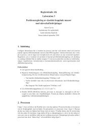
Perstorp. The site consists of 10 production areas. The products
of the 10 areas at the site are here denoted product 1-10
for area 1-10 respectively. Internal buffer tanks exist for
products 1-5. A flowchart of the product flow at the site is
shown in Figure 1. The utilities that are used at site Stenungsund
are listed below. Disturbance limits for these utilities
have been determined by speaking to operators and other
Figure 1. Product flow at site Stenungsund.

staff at the site and looking into historical databases and log
books.
• Steam (High pressure (HP) and middle pressure (MP))
• Cooling water (Cooling water and four cooling fans)
• Electricity
• Water treatment
• Combustion of tail gas (Flare and two combustion devices)
• Nitrogen
• Water (Feed water)
• Compressed air (Instrument air)
• Vacuum system
Atableshowingwhichutilitiesthatareneededateach
area is shown in Table 1. Here some utilities have been divided
into sub-utilities.
Table 1. Utilities required at areas at site Stenungsund.
1 2 3 4 5 6 7 8 9 10
Steam HP x x x x
Steam MP x x x x x x x x
Cooling water x x x x x x x x x x
Cooling fan 1 x
Cooling fan 2 x
Cooling fan 3 x
Cooling fan 7 x
Electricity x x x x x x x x x x
Water treatment x x x x x x x x
Flare x x x x x x x
Combustion device 7 x
Combustion device 9 x
Nitrogen x x x x x x x x x x
Feed water x x x x x x
Instrument air x x x x x x x x x x
Vacuum system x x x x x x x x x x
The time period August 1, 2007 to July 1, 2010 is considered,
and the data has a sampling interval of 1 minute.
There has been one planned stop during the time period,
from September 15 to October 8, 2009. Data from this time
period is not included in the computations.
6.2 Compute utility and area availabilities
Availabilities for all utilities can be computed directly using
measurement data and the disturbance limits set in the previous
step. In Table 2, the resulting utility availabilities at
site Stenungsund for the time period August 1, 2007 to July
1, 2010 are listed.
The direct and total area availabilities for all production
areas are computed using utility measurement data, Table 1
and the flowchart of the product flow in Figure 1. The result
is given in Table 3.
6.3 Estimate revenue loss due to disturbances in utilities
To estimate the revenue loss due to disturbances in utilities,
an estimate of the flows to the market of all products
is needed. The flows to the market are assumed to be constant
over the time period. The flow to market of a product
at maximum production is estimated as the difference of the
production of the product and the inflows of the product to
Table 2. Utility availabilities at site Stenungsund.
Utility Availability
(%)
Flare 100.00
Vacuum system 100.00
Water treatment 100.00
Instrument air 99.98
Cooling fan 7 99.88
Nitrogen 99.87
Electricity 99.28
Feed water 98.91
HP steam 98.55
Cooling fan 1 96.82
Cooling fan 2 96.82
Cooling fan 3 96.82
MP steam 96.76
Combustion device 9 96.06
Combustion device 7 94.18
Cooling water 92.33
Table 3. Availabilities of areas at site Stenungsund.
Direct Total
Area availability availability
(%) (%)
1 84.45 84.45
2 84.45 84.45
3 84.45 84.45
4 87.24 84.45
5 87.24 84.45
6 87.24 84.45
7 82.37 80.27
8 89.03 83.71
9 83.99 81.46
10 89.60 89.60
downstream areas. If the estimated flow to the market becomes
less than zero, it is set to zero and the maximum production
of the area(s) downstream is adjusted to correspond
the maximum production of the upstream area. The maximum
production rates of all products at site Stenungsund are
available, but not the corresponding inflows to these areas.
The inflows are estimated from the maximum productions in
the areas via a conversion factor, denoted yij for the conversion
between product i and j. Theconversionfactorshave
been obtained from personnel at the site. An estimation of
the flows to the market becomes
q m 1 =max(0,q1 − q4y14 − q5y15 − q6y16) (1)
q m 2 =max(0,q2 − q6y26) (2)
q m 3 =max(0,q3 − q7y37) (3)
q m 4 =max(0,q4 − q8y48) (4)
q m 5 =max(0,q5 − q9y59) (5)
q m i = qi, i =6, 7, 8, 9, 10 (6)
where qi is the maximum production rate of area i in the
unit volume/time.

The direct revenue loss, J dir ,duetoutilitiesistheloss
each utility causes directly, because of reduced production
in the areas that require the utility. This loss may be estimated
directly from the utility availabilities, the flows to the
market, and the contribution margins of the products produced
in the areas that require the utility. We get the direct
loss
J dir
u =(1− U av
u ) ttot
�
i
q m i pi
for utility u, whenareasi require this utility and U av
u is the
availability of utility u. pi denotes the contribution margin
for product i in the unit profit/volume and ttot the total duration
of the considered time period. For this case study, there
are 1 501 921 sampling points (planned stop not included),
which gives a total time of about 25 000 hours of the entire
time period.
The total revenue loss due to utilities includes both the
direct revenue loss and the indirect revenue loss due to reduced
production in areas that are dependent on the areas
that require the utility. Here, only downstream effects of
disturbances are considered, since a product of an upstream
area at the site often can be sold on the market when it cannot
be delivered to its downstream area(s). At site Stenungsund,
buffer tanks for products 1-5 may thus be utilized to
reduce the indirect loss of products 4-9.
For areas with more than one downstream area, a decision
must be taken regarding which areas that should be prioritized
when the available buffer volume is not enough to
provide all areas during the entire disturbance duration. The
actual decisions, taken by the operators at the site at the occurrences
of the disturbances, are not known for the entire
set of measurement data. Also, since the real site does not
have on/off production, the areas were not shut down entirely
due to small utility disturbances. To get an estimate of
the revenue loss for the selected time period, the suggestion
is to apply the same decision rule at each disturbance detected
in the measurement data. At site Stenungsund, only
the buffer tank for product 1 has more than one downstream
area. Here, the choice has been made to prioritize downstream
areas in order area 5, area 6, area 4, based on profitability
measured as profit per time unit for the entire production
lines downstream of the buffer tank.
Disturbances in different utilities affect areas at site Stenungsund
according to Table 1. Disturbances in utilities that
affect an area upstream of a buffer tank, but not all downstream
areas of the tank can be handled using the available
volume of the buffer tank. At site Stenungsund, the utilities
that cause such disturbances are middle pressure (MP)
steam, cooling fans in area 1-3 and feed water. Downstream
areas might or might not be able to run during the entire
failure, depending on the flows that are demanded by these
areas, the duration of the disturbance and the level of the
buffer tank at the occurrence of the disturbance. For disturbances
in MP steam, cooling fans in area 1-3 and feed
water, the time ti that the downstream area i can run during
afailureoftheupstreamareaofdurationtd is given by:
MP steam
t8 =max � 0, min � td,V4/q in
8
Cooling fan 1
t5 =max � 0, min � td,V1/q in
5
��
��
t6 =max � 0, min � td, � V1 − tdq in
5
� �� in1
/q6 (9)
t4 =max � 0, min � td, � V1 − td(q in
5 + q in1
6 ) � /q in��
4 (10)
Cooling fan 2
t6 =max � 0, min � td,V2/q in2
6
Cooling fan 3
t7 =max � 0, min � td,V3/q in
7
��
��
Feed water
t6,1 =max � 0, min � td,V1/q in1��
6
t6,2 =max � 0, min � td,V2/q in2��
6
t7 =max � 0, min � td,V3/q in��
7
t9 =max � 0, min � td,V5/q in��
9
(7)
(8)
(11)
(12)
(13)
(14)
(15)
(16)
where Vi is the buffer volume in the buffer tank for product
i at the start of the failure, and qin j the demanded inflow for
area j to be able to produce, given by qin j = qjyij,asin(1)-
(5). For feed water failures that affect area 6, simultaneous
failures in area 1 and 2 are taken into account to get t6.
The indirect revenue loss J id
u due to utility u can then be
estimated as
J id
u = � �
(td − ti)q m i pi
td
i
for all areas i downstream of buffer tanks, and all disturbance
durations td for the utility during the entire time period.
ti is the time area i can run during each disturbance,
and is given by (7)-(16).
Summarizing both direct revenue losses and indirect
losses at buffer tanks we get an estimate of the total loss
J tot dir id
u = Ju + Ju due to utility u. InTable4,utilitiesare
ordered according to the revenue loss they cause, starting
with the utility that causes the greatest loss.
6.4 Reduce revenue loss due to future disturbances in utilities
On/off production modeling including buffer tanks gives
two strategies for decreasing the revenue loss due to utilities.
The first is to choose good stationary buffer tank levels
(proactive disturbance management), and the second to
control the product flow properly at the occurrence of a disturbance
(reactive disturbance management). Below, these
two strategies are discussed.
Choice of buffer tank levels Good choices of stationary
buffer tank levels can ensure that the site can run even at
afailureinoneormoreareas.Inthiscasestudy,ithasbeen
chosen to only consider downstream effects of a disturbance

Table 4. Utilities ordered according to the loss they cause.
Direct loss Total loss
Cooling water Cooling water
MP steam MP steam
Combustion device 9 Cooling fan 1
Combustion device 7 Feed water
Cooling fan 1 Combustion device 9
Electricity Combustion device 7
HP steam Electricity
Feed water HP steam
Nitrogen Nitrogen
Cooling fan 3 Cooling fan 3
Cooling fan 2 Cooling fan 2
Instrument air Instrument air
Cooling fan 7 Cooling fan 7
Flare Flare
Vacuum system Vacuum system
Water treatment Water treatment
upstream of a buffer tank. Thus, only lower constraints on
the buffer tank levels will be imposed, and there will be a
trade-off between handling as many failures as possible and
minimizing inventory at the site. This work does not focus
on computing the costs of the inventories to achieve the optimal
trade-off between utility disturbance management and
cost of inventory. Here, another strategy for choosing the
trade-off between these is used, which is described below.
Optimal choice of inventory is discussed in e.g. Silver et al.
(1998), Newhart et al. (1993) and Hopp et al. (1989).
Choosing the buffer tank levels to handle the longest disturbance
durations for utilities will often give unneccesarily
high buffer tank levels at normal operation, since disturbances
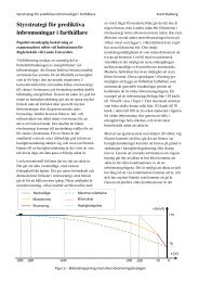
of such long durations often are very uncommon. A
suggestion is to choose the levels so that a certain percentage
of all disturbances in utilities are handled. In Figure 2, the
levels that correspond to handling 90 % of all disturbances
in utilities at site Stenungsund are given, based on measurement
data from the considered time period. As a comparison,
the average buffer tank levels over the considered time
period is shown in the figure. It can be seen that the average
buffer tank levels over the selected time period are well
above the levels required to handle 90 % of all disturbances
in utilities. However, the buffer levels are not chosen only
to handle disturbances in utilities, but to handle all disturbances
at the site and to provide inventory of products to be
Figure 2. Buffer tank levels at site Stenungsund.
sold to the market. This must be taken into account to evaluate
if the buffer tank levels are appropriately chosen. The
constraints from disturbances in utilities give one piece that
has to be taken into account when choosing desired buffer
tank levels.
If upstream disturbances also are taken into account, disturbances
that affect a downstream area of a buffer tank, but
not all upstream areas, will impose high-level constraints on
some buffer tanks.
Control of the product flow At the occurrence of a disturbance,
a decision must be taken on how to control the product
flow if the area that suffers a failure has more than one
downstream area. A guideline for how to control the product
flow when a disturbance occurs is obtained from the simple
on/off site model with buffer tanks, where the suggestion is
to run the areas according to equations (7)-(16). Since the
disturbance duration td is not known a priori, td is replaced
by the estimated disturbance duration test in the equations.
The suggestion in Lindholm (2011) is to let the operators
at the site estimate the disturbance duration at the occurrence
of a disturbance. This suggestion of the control of
the product flow can be recomputed if the estimatie of the
disturbance time changes.
Over time, contribution margins for different products
could change, which makes it necessary to change the prioritization
order of areas. Also, the order can be chosen
differently depending on what is the most suitable measure
of profitability at the site. Measures that could be used are
profit/volume or profit/time.
6.5 Comparison of on/off production modeling with and
without buffer tanks
The direct revenue loss caused by disturbances in utilities
is the same for on/off production with and without buffer
tanks. In Table 5, utilities are ordered according to the estimate
of the total revenue loss they cause for on/off production
with and without buffer tanks, in descending order.
Table 5. Utilities ordered according to the total revenue
loss they cause.
On/off On/off with buffer tanks
Cooling water Cooling water
MP steam MP Steam
Cooling fan 1 Cooling fan 1
Feed water Feed water
Combustion device 9 Combustion device 9
Combustion device 7 Combustion device 7
Electricity Electricity
HP steam HP steam
Cooling fan 2 Nitrogen
Cooling fan 3 Cooling fan 3
Nitrogen Cooling fan 2
Instrument air Instrument air
Cooling fan 7 Cooling fan 7
Flare Flare
Vacuum system Vacuum system
Water treatment Water treatment

Because of the reduction of the indirect revenue losses
caused by MP steam, cooling fans 1-3 and feed water, the
ordering is changed when including buffer tanks in the site
model. Table 6 shows how much the revenue losses caused
by these utilities decrease when internal buffer tanks are utilized.
In the table, the utilities are ordered according to the
reduction of the revenue loss in money.
Table 6. Decrease of revenue losses when including buffer
tanks.
Utility Decrease (%)
Cooling fan 1 54
Cooling fan 2 86
Cooling fan 3 80
MP steam 7
Feed water 4
7. Conclusions and Future work
The case study at Perstorp presented in this paper gives ordering
of utilities at the site according to an estimate of the
loss of revenue they cause, using an on/off modeling approach
with buffer tanks between areas. It also illustrates the
influence of buffer tanks at the site, by showing how much
the loss in revenue caused by disturbances in utilities can be
reduced by introducing buffer tanks between the areas.
Strategies for reducing the revenue loss due to utility disturbances
are suggested for the Stenungsund site. It should
be noted that only disturbances in utilities have been considered.
This is only one piece of the entire picture, where
also market conditions, cost of inventories and other disturbances
must be taken into account. This case study shows
which constraints disturbances in utilities place on buffer
tank levels and product flow control. The aim of this study
was not to achieve the optimal trade-off between utility disturbance
management and inventory costs.
The on/off production modeling approach including
buffer tanks should give more accurate estimates of the
losses that are caused by utilities at a site than the on/off
model without buffer tanks. However, areas are still modeled
as on or off, and thus the site model does not adequately
reflect the actual production. To catch more of the variability,
the site should be modeled using a continuous production
model. Continuous production modeling of a site is
currently being investigated, and will also be applied to Perstorp’s
site at Stenungsund. With continuous production,
more elaborate reactive disturbance management strategies
may be obtained, that gives real-time advise to operators on
how to control the product flow at the occurrence of a disturbance.
Acknowledgments
This research was performed within the framework of the
Process Industrial Centre at Lund University (PIC-LU),
which is supported by the Swedish Foundation for Strategic
Research (SSF).
References
Bakhrankova, K. (2010). Decision support system for continuous
production. Industrial Management & Data Systems, 110(4),
591–610.
Bauer, M., Cox, J.W., Caveness, M.H., Downs, J.J., and Thornhill,
N.F. (2007). Nearest neighbors methods for root cause analysis
of plantwide disturbances. Ind. Eng. Chem. Res,46,5977–5984.
Faanes, A. and Skogestad, S. (2003). Buffer tank design for acceptable
control performance. Ind. Eng. Chem. Res., 42(10),
2198–2208.
Hopp, W.J., Pati, N., and Jones, P.C. (1989). Optimal inventory
control in a production flow system with failures. International
Journal of Production Research, 27(8),1367–1384.
Kano, M. and Nakagawa, Y. (2008). Data-based process monitoring,
process control, and quality improvement: Recent developments
and applications in steel industry. Computers & Chemical
Engineering, 32(1-2),12–24.
Lindholm, A. (2011). A method for improving plant availability
with respect to utilities using buffer tanks. In proceedings of the
IASTED International Conference on Modeling, Identification
and Control (MIC 2011), Innsbruck, Austria,378–383.
Lindholm, A., Carlsson, H., and Johnsson, C. (2011a). Estimation
of revenue loss due to disturbances on utilities in the process
industry. In proceedings of the 22 nd Annual Conference of
the Production and Operations Management Society (POMS),
Reno, NV, USA.
Lindholm, A., Carlsson, H., and Johnsson, C. (2011b). A general
method for handling disturbances on utilities in the process industry.
In proceedings of the 18 th World Congress of the International
Federation of Automatic Control (IFAC), Milano, Italy,
2761–2766.
Maia, L.O.A., de Carvalho, L.A.V., and Qassim, R.Y. (1995). Synthesis
of utility systems by simulated annealing. Computers &
Chemical Engineering, 19(4),481–488.
Maia, L.O.A. and Qassim, R.Y. (1997). Synthesis of utility systems
with variable demands using simulated annealing. Computers &
Chemical Engineering, 21(9),947–950.
Newhart, D.D., Stott Jr., K.L., and Vasko, F.J. (1993). Consolidating
product sizes to minimize inventory levels for a multi-stage
production and distribution system. The Journal of the Operational
Research Society, 44(7),637–644.
Niebert, P. and Yovine, S. (1999). Computing optimal operation
schemes for multi batch operation of chemical plants. VHS deliverable.
Draft.
Papoulias, S.A. and Grossmann, I.E. (1983). A structural optimization
approach in process synthesis–ı : Utility systems. Computers
& Chemical Engineering, 7(6),695–706.
Qin, S. (1998). Control performance monitoring - a review and
assessment. Computers & Chemical Engineering, 23,173–186.
Silver, E.A., Pyke, D.F., and Peterson, R. (1998). Inventory Management
and Production Planning and Scheduling. Wiley,New
York.
Thornhill, N.F., Xia, C., Howell, J., Cox, J., and Paulonis, M.
(2002). Analysis of plant-wide disturbances through data-driven
techniques and process understanding. In proceedings of the
15 th IFAC World Congress, Barcelona.