Design and Implementation of Object-Oriented ... - Automatic Control
Design and Implementation of Object-Oriented ... - Automatic Control
Design and Implementation of Object-Oriented ... - Automatic Control

Create successful ePaper yourself
Turn your PDF publications into a flip-book with our unique Google optimized e-Paper software.
<strong>Design</strong> <strong>and</strong> <strong>Implementation</strong> <strong>of</strong><br />
<strong>Object</strong>-<strong>Oriented</strong> Model Libraries<br />
using Modelica<br />
Hubertus Tummescheit<br />
<strong>Automatic</strong> <strong>Control</strong>
<strong>Design</strong> <strong>and</strong> <strong>Implementation</strong> <strong>of</strong><br />
<strong>Object</strong>-<strong>Oriented</strong> Model Libraries using Modelica
<strong>Design</strong> <strong>and</strong> <strong>Implementation</strong> <strong>of</strong><br />
<strong>Object</strong>-<strong>Oriented</strong> Model Libraries<br />
using Modelica<br />
Hubertus Tummescheit<br />
Department <strong>of</strong> <strong>Automatic</strong> <strong>Control</strong><br />
Lund Institute <strong>of</strong> Technology<br />
Lund, August 2002
Department <strong>of</strong> <strong>Automatic</strong> <strong>Control</strong><br />
Lund Institute <strong>of</strong> Technology<br />
Box 118<br />
SE-221 00 LUND<br />
Sweden<br />
ISSN 0280–5316<br />
ISRN LUTFD2/TFRT–1063–SE<br />
c2002 by Hubertus Tummescheit. All rights reserved.<br />
Printed in Sweden by Bloms i Lund Tryckeri AB.<br />
Lund 2002
Contents<br />
Preface . . . . . . . . . . . . . . . . . . . . . . . . . . . . . . . . . 7<br />
Acknowledgments . . . . . . . . . . . . . . . . . . . . . . . . . . 7<br />
1. Introduction . . . . . . . . . . . . . . . . . . . . . . . . . . . . 9<br />
1.1 Why Modeling is Important . . . . . . . . . . . . . . . . . 9<br />
1.2 Outline <strong>and</strong> Contributions . . . . . . . . . . . . . . . . . 11<br />
1.3 Purpose <strong>of</strong> Modeling . . . . . . . . . . . . . . . . . . . . . 13<br />
1.4 A Turbine System . . . . . . . . . . . . . . . . . . . . . . 15<br />
1.5 How the Work Developed . . . . . . . . . . . . . . . . . . 16<br />
2. Modeling Techniques . . . . . . . . . . . . . . . . . . . . . . . 19<br />
2.1 Representation <strong>of</strong> Dynamics . . . . . . . . . . . . . . . . 19<br />
2.2 Model Libraries . . . . . . . . . . . . . . . . . . . . . . . . 39<br />
2.3 Validation <strong>and</strong> Verification . . . . . . . . . . . . . . . . . 42<br />
2.4 Physics Based Model Reduction . . . . . . . . . . . . . . 44<br />
2.5 Modeling Tools . . . . . . . . . . . . . . . . . . . . . . . . 49<br />
3. The Modelica Language . . . . . . . . . . . . . . . . . . . . . 52<br />
3.1 Introduction . . . . . . . . . . . . . . . . . . . . . . . . . . 52<br />
3.2 Key Features <strong>of</strong> Modelica . . . . . . . . . . . . . . . . . . 54<br />
3.3 Modelica Basics . . . . . . . . . . . . . . . . . . . . . . . . 56<br />
3.4 Annotations <strong>and</strong> Pragmas . . . . . . . . . . . . . . . . . . 68<br />
4. Physical Models for Thermo-Hydraulics . . . . . . . . . . 71<br />
4.1 Introduction . . . . . . . . . . . . . . . . . . . . . . . . . . 71<br />
4.2 Fluid Transport Equations . . . . . . . . . . . . . . . . . 73<br />
4.3 Balance Equations . . . . . . . . . . . . . . . . . . . . . . 75<br />
4.4 The General Transport Equation . . . . . . . . . . . . . . 84<br />
4.5 Thermodynamic Equations <strong>of</strong> State . . . . . . . . . . . . 84<br />
4.6 Choice <strong>of</strong> Dynamic State Variables . . . . . . . . . . . . 89<br />
4.7 Turbines <strong>and</strong> Valves . . . . . . . . . . . . . . . . . . . . . 96<br />
4.8 Pumps <strong>and</strong> Compressors . . . . . . . . . . . . . . . . . . 99<br />
4.9 Chemical Reactions . . . . . . . . . . . . . . . . . . . . . 101<br />
5
Contents<br />
4.10 Solid Structures . . . . . . . . . . . . . . . . . . . . . . . 102<br />
4.11 Moving Boundary Models . . . . . . . . . . . . . . . . . . 104<br />
4.12 Void Distribution . . . . . . . . . . . . . . . . . . . . . . . 113<br />
5. The ThermoFluid Library . . . . . . . . . . . . . . . . . . . . 121<br />
5.1 Introduction . . . . . . . . . . . . . . . . . . . . . . . . . . 121<br />
5.2 Basic Ideas . . . . . . . . . . . . . . . . . . . . . . . . . . 124<br />
5.3 <strong>Control</strong> Volumes <strong>and</strong> Flow Models . . . . . . . . . . . . . 127<br />
5.4 <strong>Object</strong>-Orientation in ThermoFluid . . . . . . . . . . . . 129<br />
5.5 Interfaces . . . . . . . . . . . . . . . . . . . . . . . . . . . 136<br />
5.6 Base Models . . . . . . . . . . . . . . . . . . . . . . . . . . 140<br />
5.7 Partial Components . . . . . . . . . . . . . . . . . . . . . 151<br />
5.8 Component Models . . . . . . . . . . . . . . . . . . . . . . 154<br />
5.9 Examples . . . . . . . . . . . . . . . . . . . . . . . . . . . 159<br />
5.10 ThermoFluid Applications . . . . . . . . . . . . . . . . . . 162<br />
5.11 Comparison with Domain Specific Tools . . . . . . . . . . 170<br />
5.12 Summary . . . . . . . . . . . . . . . . . . . . . . . . . . . 176<br />
6. <strong>Design</strong> <strong>of</strong> Model Libraries . . . . . . . . . . . . . . . . . . . 178<br />
6.1 Introduction . . . . . . . . . . . . . . . . . . . . . . . . . . 178<br />
6.2 Means for Library Structuring . . . . . . . . . . . . . . . 180<br />
6.3 <strong>Design</strong> Patterns for Modeling . . . . . . . . . . . . . . . . 191<br />
6.4 Structural <strong>Design</strong> Patterns . . . . . . . . . . . . . . . . . 192<br />
6.5 Numerical <strong>Design</strong> Patterns . . . . . . . . . . . . . . . . . 197<br />
6.6 Conclusions . . . . . . . . . . . . . . . . . . . . . . . . . . 204<br />
7. Recommendations for Future Work . . . . . . . . . . . . . 205<br />
7.1 Writing Models . . . . . . . . . . . . . . . . . . . . . . . . 208<br />
7.2 Model Debugging . . . . . . . . . . . . . . . . . . . . . . . 212<br />
7.3 User Interface Issues . . . . . . . . . . . . . . . . . . . . 216<br />
7.4 Partial Differential Equations . . . . . . . . . . . . . . . 217<br />
7.5 Extensions to ThermoFluid . . . . . . . . . . . . . . . . . 219<br />
7.6 Summary . . . . . . . . . . . . . . . . . . . . . . . . . . . 220<br />
8. Conclusions . . . . . . . . . . . . . . . . . . . . . . . . . . . . . 221<br />
9. References . . . . . . . . . . . . . . . . . . . . . . . . . . . . . . 224<br />
A. Glossary . . . . . . . . . . . . . . . . . . . . . . . . . . . . . . . 237<br />
B. Thermodynamic Derivatives . . . . . . . . . . . . . . . . . 242<br />
B.1 Fundamental Equations . . . . . . . . . . . . . . . . . . . 242<br />
B.2 Transformation <strong>of</strong> Partial Derivatives . . . . . . . . . . . 245<br />
B.3 Derivatives in the Two-Phase Region . . . . . . . . . . . 249<br />
C. Moving Boundary Models . . . . . . . . . . . . . . . . . . . . 253<br />
Mass- <strong>and</strong> Energy Balances . . . . . . . . . . . . . . . . . . . . 253<br />
D. Modelica Language Constructs . . . . . . . . . . . . . . . . 257<br />
6
Preface<br />
Preface<br />
The subject <strong>of</strong> this thesis belongs somewhere into the intersection <strong>of</strong> the<br />
disciplines <strong>of</strong> <strong>Automatic</strong> <strong>Control</strong>, Computer Science <strong>and</strong> Systems <strong>Design</strong><br />
Engineering. The thesis explores the design <strong>of</strong> object-oriented model libraries<br />
using the example <strong>of</strong> a library for thermo-fluid systems. The library<br />
is written in the new, object-oriented modeling language Modelica.<br />
During the time <strong>of</strong> the library development I was involved in the design <strong>of</strong><br />
the Modelica language from an early stage. It was a great pleasure for me<br />
to participate in the design <strong>of</strong> the language <strong>and</strong> to pioneer its use. The<br />
enthusiasm <strong>of</strong> the members <strong>of</strong> the Modelica <strong>Design</strong> group for modeling<br />
<strong>and</strong> simulation problems has been contagious.<br />
The task <strong>of</strong> writing an interdisciplinary thesis is challenging in terms<br />
<strong>of</strong> finding the right level <strong>of</strong> detail for readers with widely differing background<br />
knowledge. Some readers may wish to skip parts <strong>of</strong> the thesis that<br />
are either not interesting or well known to them. Readers with a special<br />
interest in thermo-fluid models should read Chapter 4, people which are<br />
curious about the ThermoFluid library should read Chapter 5 <strong>and</strong> modelers<br />
looking for ideas about object-oriented library design in general may<br />
find Chapter 6 interesting.<br />
Acknowledgments<br />
Writing a thesis is a project that lives from the exchange <strong>of</strong> ideas <strong>and</strong><br />
lively discussions. Many people have helped me in producing this thesis,<br />
through discussions <strong>and</strong> close cooperation in several projects <strong>and</strong> by being<br />
joyful colleagues, good friends <strong>and</strong> keeping my spirits up.<br />
First <strong>of</strong> all I have to thank the coordinated efforts <strong>of</strong> three people who<br />
made me come to Lund <strong>and</strong> stay here: Sven Erik Mattsson who invited me<br />
<strong>and</strong> got me started, Jonas Eborn for making the team work such a nice<br />
experience <strong>and</strong> Karl Johan Åström who convinced me to stay <strong>and</strong> do my<br />
PhD in Lund. Thanks for that, I have a great time here. The collaboration<br />
with Jonas has been a source <strong>of</strong> inspiration during the whole project.<br />
I am glad to express my sincere gratitude to Karl Johan Åström. His<br />
constructive criticism on several chapters <strong>of</strong> the manuscript helped to improve<br />
its readability. He has created the necessary conditions for a very<br />
stimulating research atmosphere <strong>and</strong> is a consistent source <strong>of</strong> enthusiasm.<br />
It has been a great pleasure <strong>and</strong> privilege to learn from you. Many<br />
thanks to my other supervisor Anders Rantzer. He has the gift <strong>of</strong> always<br />
asking the most relevant <strong>and</strong> interesting questions. His incessant dem<strong>and</strong><br />
for new chapters <strong>of</strong> the thesis <strong>and</strong> valuable comments on the manuscript<br />
helped a lot getting this work done. Many thanks also to other senior<br />
7
staff at the department to acquire the funding for many graduate students.<br />
Many thanks to all who pro<strong>of</strong>read parts <strong>of</strong> the manuscript <strong>and</strong><br />
gave feedback: Sven Erik Mattsson, Jakob Munch Jensen, Jonas Eborn,<br />
Godela Rossner, Karl Erik Arzén <strong>and</strong> Johan Åkesson. Special thanks to<br />
my mother for correcting my English under time pressure.<br />
I also wish to thank Falko Jens Wagner for the good time we had<br />
working together with the ThermoFluid library <strong>and</strong> Jakob Munch Jensen<br />
for many stimulating discussions, good laughs, interesting joint work <strong>and</strong><br />
cultural expeditions to Copenhagen’s Theaters <strong>and</strong> Jazz Clubs.<br />
Special thanks go to the people at Dynasim AB who provided us with<br />
new versions <strong>of</strong> Dymola as soon as we tested the latest additions to the<br />
Modelica language. Particular thanks to Hans Olsson for his enthusiastic<br />
greetings when receiving a bug report or feature request on the phone.<br />
Special thanks also to all members <strong>of</strong> the Modelica Association. The discussions<br />
about modeling <strong>and</strong> language design in a group with such a broad<br />
background has been a valuable source <strong>of</strong> insight <strong>and</strong> ideas. I appreciated<br />
the combination <strong>of</strong> intensive technical discussions <strong>and</strong> a friendly, relaxed<br />
atmosphere around them.<br />
I wish to thank the Masters students that I supervised, Olaf Bauer,<br />
Antonio Gómez Pérez <strong>and</strong> Staffan Haugwitz, for many good ideas <strong>and</strong> contributions.<br />
Olaf has done valuable base work for fluid property functions<br />
with his Maple-package for thermodynamic derivatives.<br />
I am grateful to my colleagues at the Department who create a friendly<br />
<strong>and</strong> inspiring atmosphere. I specially would like to thank the following:<br />
Eva Schildt, Britt-Marie Mårtensson <strong>and</strong> Agneta Tuszynski for keeping<br />
our spirits up <strong>and</strong> running the unnoticed background work, Leif Andersson<br />
<strong>and</strong> Anders Blomdell for keeping the computers in good health, Sven<br />
Hedlund for his enthusiastic advertisements for running in Skrylle, Magnus<br />
Gäfvert for hints about interesting music <strong>and</strong> Andrey Ghulchak for<br />
organizing the “inspirationsfika”.<br />
Many thanks to the Sunday dinner gang for many nice evenings, lots <strong>of</strong><br />
ice-cream, never rejecting a Malt <strong>and</strong> for almost always doing the dishes<br />
before leaving: Andrey, Shi-Lin, Ari, Beatrice, Stephane, Jenny, Stefan,<br />
Maru <strong>and</strong> the many guests who came during their visits in Lund.<br />
This project has jointly been supported by Sydkraft AB under the<br />
project name “Modelling <strong>and</strong> <strong>Control</strong> for Energy Systems” <strong>and</strong> by the<br />
National Board for Industrial <strong>and</strong> Technical Development (NUTEK) programme<br />
“Complex Systems”, Dnr 96-10653. Their financial support is<br />
gratefully acknowledged.<br />
8
1<br />
Introduction<br />
Abstract<br />
This chapter provides background about modeling <strong>of</strong> physical systems<br />
in order to explain the need for better tools <strong>and</strong> languages for<br />
modeling. It is motivated that an important part <strong>of</strong> engineering knowhow<br />
is encoded in system models. This knowledge needs to be stored<br />
in a formal <strong>and</strong> reusable way.<br />
1.1 Why Modeling is Important<br />
Mathematical models are compact representations <strong>of</strong> knowledge. Probably<br />
the most important but intangible advantage <strong>of</strong> modeling is the insight<br />
<strong>and</strong> increased underst<strong>and</strong>ing that the process <strong>of</strong> modeling gives about a<br />
system. Knowledge is much easier to communicate in the form <strong>of</strong> a mathematical<br />
model than with a textual description. Engineering knowledge<br />
<strong>and</strong> education is to a large extent based on models in different domains.<br />
When this knowledge is made available to the engineering design process,<br />
it helps a great deal to increase safety, quality <strong>and</strong> economy <strong>of</strong> that system.<br />
Modeling is a major part in any engineering development. A model<br />
that is executable in a simulation program is much easier <strong>and</strong> safer to<br />
work with than the real system. This has been summarized very well by<br />
an executive at one <strong>of</strong> the largest companies in the process industry:<br />
Modeling <strong>and</strong> simulation technologies are keys to achieve<br />
manufacturing excellence <strong>and</strong> to assess risk in unit operations.<br />
As we make our plant more flexible to respond to business opportunities,<br />
efficient modeling <strong>and</strong> simulation techniques will<br />
become commonly used tools.<br />
Ralph P. Schlenker, Exxon Chemical<br />
In todays engineering practice, model based analysis, simulation <strong>and</strong><br />
design are major pillars in the development <strong>of</strong> advanced technical prod-<br />
9
Chapter 1. Introduction<br />
Level <strong>of</strong> Detail<br />
System<br />
requirements<br />
Architectural design &<br />
system functional design<br />
Preliminary<br />
feature design<br />
The <strong>Design</strong> Arch<br />
Realization<br />
Detailed feature design Component verification<br />
<strong>and</strong> implementation<br />
Specification<br />
<strong>Design</strong> <strong>Design</strong> Refinement<br />
Next Product Generation<br />
Experience Feedback<br />
Verification Integration Calibration<br />
Version <strong>and</strong> Configuration Management<br />
Documentation<br />
Subsystem level integration<br />
<strong>and</strong> verification<br />
System level integration, test<br />
calibration <strong>and</strong> verification<br />
Product verification<br />
<strong>and</strong> deployment<br />
Maintenance<br />
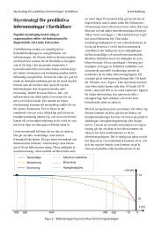
Figure 1.1 <strong>Design</strong> arch <strong>of</strong> product development <strong>and</strong> life cycle. A similar scheme<br />
is sometimes referred to as design-V.<br />
ucts. Cost savings achieved by avoiding possibly destructive “smoke tests”<br />
<strong>of</strong> expensive hardware <strong>and</strong> by doing this test as a model based computer<br />
simulation instead, are a strong driving force for model development. Development<br />
cycles for new technical products are shortened by making developments<br />
in parallel instead <strong>of</strong> sequential. Emulating a not-yet-existing<br />
piece <strong>of</strong> hardware on a computer, <strong>of</strong>ten in a hardware-in-the-loop (HIL)<br />
configuration, is a st<strong>and</strong>ard technique for achieving concurrent engineering.<br />
HIL needs models which are not only accurate representations <strong>of</strong> reality,<br />
but also fulfill stringent performance criteria. The simulation must<br />
be executed in real time, otherwise it is not possible to emulate reality to<br />
a degree that allows meaningful tests, e. g., <strong>of</strong> control equipment.<br />
Figure 1.1 illustrates the typical phases <strong>of</strong> development <strong>of</strong> a technical<br />
product. Almost all phases can to some extent benefit from modeling<br />
<strong>and</strong> simulation. The models which are needed in the phases <strong>of</strong>ten have<br />
different requirements: the change in the level <strong>of</strong> detail leads to different<br />
models. Modeling language features that help reuse in concurrent engineering<br />
<strong>and</strong> simplify model reduction are important. It is even useful to<br />
be able to keep the structure but exchange the underlying model completely.<br />
On the right h<strong>and</strong> side <strong>of</strong> the design arch, hardware-in-the-loop<br />
is a well known means to reduce testing cost. The performance requirements<br />
are <strong>of</strong>ten difficult to achieve. Reuse <strong>of</strong> models, both throughout the<br />
design process <strong>and</strong> for the next-generation product, is an important factor<br />
to reduce modeling <strong>and</strong> simulation costs.<br />
10
1.2 Outline <strong>and</strong> Contributions<br />
1.2 Outline <strong>and</strong> Contributions<br />
This thesis discusses the development <strong>of</strong> an object-oriented model library<br />
for thermo-fluid systems with focus on the structuring <strong>and</strong> reuse <strong>of</strong> models.<br />
The development was done in parallel to the development <strong>of</strong> the underlying<br />
modeling language, Modelica TM [Modelica Association, 2002a] which<br />
is specifically designed to facilitate model reuse. This parallel development<br />
closed the feedback loop between model development <strong>and</strong> modeling<br />
language development in a very fruitful way. New concepts in the language<br />
were implemented in the library, experience from the use <strong>of</strong> the<br />
new concepts was used to refine the language definition <strong>and</strong> make it more<br />
powerful <strong>and</strong> easier to use in the next iteration <strong>of</strong> the language. This interplay<br />
<strong>of</strong> serious model development, structuring <strong>of</strong> models for reuse <strong>and</strong><br />
language design by experts in many engineering domains has helped to<br />
shape Modelica 1 into its current form. The process is not finished: mathematical<br />
modeling <strong>of</strong> systems is <strong>and</strong> will remain to be a challenging activity.<br />
The main contributions in the thesis are the following:<br />
• Model library design. The desire to develop object-oriented, reusable<br />
physical models has been a driving force <strong>of</strong> this work which<br />
started before the idea <strong>of</strong> Modelica was born. The first library was<br />
written in the SMILE language, [Mühlthaler, 2000], jointly developed<br />
by GMD FIRST <strong>and</strong> the Technical University <strong>of</strong> Berlin. The<br />
Smile language was oriented more specifically towards the simulation<br />
<strong>of</strong> power plants <strong>and</strong> was successfully used in a fluidized bed<br />
combined heat <strong>and</strong> power plant [Buse, 2001] <strong>and</strong> a combined solar<br />
thermal power plant [Tummescheit <strong>and</strong> Pitz-Paal, 1997]. The<br />
scope <strong>of</strong> the library was broadened to general thermo-fluid systems<br />
when it was redesigned in Modelica. Experiences were combined<br />
with those gained in the development <strong>of</strong> the K2 library developed<br />
at Lund University, [Eborn <strong>and</strong> Nilsson, 1996; Eborn, 1998]. Earlier<br />
stages <strong>of</strong> this work were presented in [Tummescheit <strong>and</strong> Eborn,<br />
1998; Eborn et al., 1999; Tummescheit et al., 2000; Tummescheit<br />
<strong>and</strong> Eborn, 2002; Tummescheit, 2000a; Tummescheit, 2000b].<br />
• Modelica language design. The design <strong>of</strong> the Modelica language<br />
was a joint effort with contributions from many experts in several<br />
engineering domains, computer science <strong>and</strong> numerical mathematics.<br />
It was a collaborative development that I had the pleasure to participate<br />
in. An important aspect <strong>of</strong> the Modelica evolution was the<br />
tight feedback loop between model language design <strong>and</strong> use <strong>of</strong> Modelica<br />
in real world problems. My special interests here were high<br />
1 The TM -sign is omitted from now on to improve readability.<br />
11
Chapter 1. Introduction<br />
level parameters (also called class parameters) <strong>and</strong> efforts to make<br />
sure that external functions written in C or FORTRAN are easy to<br />
integrate. The result <strong>of</strong> this work is published in Modelica specification<br />
[Modelica Association, 2002b]. An early design stage <strong>of</strong> class<br />
parameters in Modelica is presented in [Tummescheit et al., 1997].<br />
• Models for thermo-fluid systems. Modeling expertise <strong>and</strong> the<br />
challenge <strong>of</strong> relevant industrial problems are a necessary background<br />
to test a model library for its usefulness. Thermo-fluid systems is my<br />
area <strong>of</strong> experience. Thermo-fluid systems have in the past been a<br />
domain where no general purpose modeling tools or languages have<br />
been available 2 . Two phase flow models like the moving boundary<br />
models presented in Chapter 4 have been <strong>of</strong> special interest. Publications<br />
on two phase flow models are [Bauer <strong>and</strong> Tummescheit,<br />
2000; Jensen <strong>and</strong> Tummescheit, 2002].<br />
• Industrial applications. An important aspect <strong>of</strong> the work was<br />
the participation in industrial modeling projects, applying the ThermoFluid<br />
library to a diverse range <strong>of</strong> real world modeling problems.<br />
Relevant projects were the modeling <strong>of</strong> combustion for automotive<br />
systems at Ford Motor Company [Tummescheit <strong>and</strong> Tiller,<br />
2000; Tiller et al., 2000], modeling <strong>of</strong> fuel cell systems at United<br />
Technologies Research Lab, modeling <strong>of</strong> a steam distribution network<br />
in a paper plant [Lindstr<strong>and</strong>, 2002] <strong>and</strong> modeling <strong>of</strong> CO2 -based<br />
refrigeration cycles. These industrial projects have given useful input<br />
to the library <strong>and</strong> the Modelica language.<br />
The thesis is organized in the following way. This chapter gives an introduction<br />
to the background <strong>and</strong> fundamental aspects <strong>of</strong> modeling <strong>and</strong><br />
simulation <strong>of</strong> systems. Chapter two presents some modeling techniques.<br />
The development <strong>of</strong> the Modelica language <strong>and</strong> a description <strong>of</strong> the key<br />
features <strong>of</strong> Modelica that are a necessary prerequisite to underst<strong>and</strong> the<br />
library design discussion follow in chapter three. Chapter four presents<br />
an overview over thermo-fluid models used in the implementation <strong>of</strong> the<br />
ThermoFluid library, described in the next chapter. Chapter six summarizes<br />
the experiences from object-oriented library design. Recommendations<br />
for future work are proposed in chapter seven <strong>and</strong> conclusions are<br />
drawn in chapter eight.<br />
2There are many simulation tools for thermo-fluid systems, but all with black box models<br />
without possibilities to create new models<br />
12
1.3 Purpose <strong>of</strong> Modeling<br />
1.3 Purpose <strong>of</strong> Modeling<br />
Modeling is a rich activity with a broad scope. The focus in this thesis is<br />
on modeling <strong>of</strong> complex technical systems. Mathematical models <strong>of</strong> systems<br />
are never done as an intellectual exercise to find the best possible<br />
mathematical representation <strong>of</strong> reality. Reality is complex, models do not<br />
<strong>and</strong> should not seek to obtain the same complexity. Models in this thesis<br />
are always done with a purpose, they are developed to answer specific<br />
questions about the system’s behavior <strong>and</strong> <strong>of</strong>ten they are restricted to<br />
certain boundary conditions or inputs to the model. As Marvin Minsky,<br />
[Minsky, 1965] put it:<br />
A model (M) for a system (S) <strong>and</strong> an experiment (E) is anything<br />
to which E can be applied to answer questions about the<br />
system S.<br />
Asking two different questions about the same systems <strong>of</strong>ten results in<br />
two different, possibly even entirely unrelated mathematical models which<br />
are best suited to answer the particular questions. It is important to realize<br />
that there is no such thing as a perfect model for a system. This is a<br />
widespread belief, based on the idea that with growing sophistication, the<br />
model eventually converges to the system. In the best case, the similarity<br />
between the behavior <strong>of</strong> the model <strong>and</strong> the modeled system increases<br />
until no difference between the two behaviors can be observed within the<br />
limits <strong>of</strong> experimental results.<br />
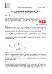
A simple illustration <strong>of</strong> a set <strong>of</strong> models with increasing sophistication<br />
are physical pictures <strong>of</strong> an object with increasing level <strong>of</strong> detail: sketch,<br />
drawing, black <strong>and</strong> white photography, color photography, hologram <strong>and</strong><br />
sculpture [Preisig, 2001], see Figure 1.2. It is interesting to note in this<br />
context that a simpler representation <strong>of</strong> reality may be more efficient<br />
in communicating the characteristic features <strong>of</strong> the system. A drawing<br />
or black <strong>and</strong> white photography may be better suited to reproduce the<br />
three dimensional features <strong>of</strong> an object than a color photography which<br />
undeniably has a larger amount <strong>of</strong> information about the real object. The<br />
term that is usually used to describe model variants <strong>of</strong> the same system<br />
is model granularity. Granularity refers to the amount <strong>of</strong> detail that a<br />
model reveals, like magnifying glasses with higher magnification reveal<br />
more spatial details <strong>of</strong> an object. In modeling for control, the magnifying<br />
glass could refer to a frequency range as well as a finer spatial subdivision.<br />
Different facets <strong>of</strong> system models may lead to models with a completely<br />
different mathematical representation.<br />
In industrial modeling practice this <strong>of</strong>ten results in heated disputes<br />
between departments about how a system model should be done <strong>and</strong> what<br />
phenomena should be included. The reason is that they want to ask differ-<br />
13
Chapter 1. Introduction<br />
(a) Sketch (b) Pencil Drawing (c) Black&White Photo<br />
Figure 1.2 Different representations <strong>of</strong> Rodins sculpture “The Thinker”. Inclusion<br />
<strong>of</strong> a holographic picture was rejected due to budget reasons.<br />
ent questions about the same system, when budgets <strong>and</strong> time schedules<br />
only allow the development <strong>of</strong> one model. This procedure <strong>of</strong>ten leads to<br />
over-modeling: models contain more details than necessary. As a result,<br />
the combined model may not be the best possible for any <strong>of</strong> the interesting<br />
questions. This typical problem demonstrates a real need for flexible<br />
modeling languages <strong>and</strong> model libraries, see [Åström, 2002]. The cost <strong>of</strong><br />
developing a model is high, therefore we want the same model to answer<br />
as many questions as possible about the system. High level models, <strong>of</strong>ten<br />
called meta-models, should provide straightforward ways to switch between<br />
different model implementations. Various terms have been used to<br />
describe this property <strong>of</strong> models. Multi-facet [Nilsson, 1993] modeling or<br />
multi-paradigm modeling [Mostermann <strong>and</strong> Vangheluwe, 2000] have been<br />
used to denote models which combine several behavioral descriptions <strong>of</strong><br />
a model into a meta-model. A meta-model representation in a computer<br />
tool should present the user with intuitive means to select the model facet<br />
that best answers a particular question.<br />
A typical problem in process engineering is when process design engineers<br />
meet control engineers <strong>and</strong> they try to settle for a common model.<br />
The design engineers want a model that optimally represents the steady<br />
state behavior <strong>of</strong> the system over the whole operating range. The control<br />
engineers want a model that represents the dynamic behavior <strong>of</strong> the sys-<br />
14
1.4 A Turbine System<br />
tem in the vicinity <strong>of</strong> the crossover frequency <strong>of</strong> the feedback loop. When<br />
controllers with integral action are used, the closed loop gain is infinity at<br />
low frequency <strong>and</strong> therefore the accuracy <strong>of</strong> the steady state model is not<br />
important. The dissimilarity <strong>of</strong> model purposes is frequently not understood<br />
by all members <strong>of</strong> an engineering team. From personal experience<br />
I can say that this problem is a major obstacle for successful teamwork<br />
in engineering projects.<br />
Webster’s dictionary defines “system” as “a regularly interacting or<br />
interdependent group <strong>of</strong> items forming a unified whole.” The key property<br />
here is the interaction <strong>of</strong> items. The notion <strong>of</strong> system thus implies that it<br />
is possible to divide the domain <strong>of</strong> interest into meaningful subunits. This<br />
observation is the starting point <strong>of</strong> all work seeking to build libraries <strong>of</strong><br />
reusable model parts. It will be a recurring theme in Chapter 6.<br />
1.4 A Turbine System<br />
A micro gas turbine system has recently been modeled in a master’s thesis<br />
project using the ThermoFluid <strong>and</strong> other Modelica libraries, [Haugwitz,<br />
2002]. It is a typical example <strong>of</strong> a multi-domain system model which<br />
demonstrates the strengths <strong>of</strong> modeling based on libraries <strong>and</strong> the need<br />
for flexible models <strong>of</strong> varying degrees <strong>of</strong> complexity.<br />
A micro turbine system is a small, compact unit for decentralized generation<br />
<strong>of</strong> electricity <strong>and</strong> heat, a so called combined heat <strong>and</strong> power plant.<br />
The recent de-regulation <strong>of</strong> the electricity market has spawned the development<br />
<strong>of</strong> these types <strong>of</strong> systems which did not exist a few years ago.<br />
Customized solutions based on micro gas turbines are actively developed<br />
now. The first generation systems where not designed for isl<strong>and</strong>ing power<br />
production during blackouts <strong>of</strong> the electrical grid, but customers request<br />
this additional feature. System models in several degrees <strong>of</strong> granularity<br />
help to speed up the development process <strong>of</strong> the more advanced controls<br />
needed for isl<strong>and</strong>ing power generation.<br />
For the particular case <strong>of</strong> this system, accurate steady state models<br />
were available but four types <strong>of</strong> dynamic models were needed:<br />
• Simple, low order models for control design.<br />
• Models that are suitable for hardware-in-the-loop tests <strong>of</strong> controllers<br />
for the main, continuous controls.<br />
• Dynamic Models for <strong>of</strong>f-line simulations <strong>and</strong> tests. These should be<br />
as accurate as possible <strong>and</strong> should be as close as possible to steady<br />
state models.<br />
15
Chapter 1. Introduction<br />
• Simple models <strong>of</strong> the gas turbine <strong>and</strong> all auxiliary systems for detailed<br />
testing <strong>of</strong> the discrete sequential controls <strong>of</strong> start-up <strong>and</strong><br />
safety procedures.<br />
All models are essentially for the same system, but with the focus on<br />
different aspects <strong>and</strong> with different questions in mind. Clearly, reusability<br />
<strong>and</strong> sharing <strong>of</strong> implementation code between these models results in a big<br />
gain in productivity.<br />
The implementation <strong>of</strong> the system model makes heavy use <strong>of</strong> many<br />
existing model libraries. Around 95 % <strong>of</strong> the total model code is from library<br />
models, the rest is divided between creation <strong>of</strong> new models <strong>and</strong><br />
composition <strong>of</strong> subsystems from libraries <strong>and</strong> new models. Without heavy<br />
code reuse, the project clearly would have been infeasible for a four month<br />
master’s thesis project. Time was too short to fulfill all wishes for modeling,<br />
but the first three <strong>of</strong> the above mentioned models could be realized<br />
<strong>and</strong> the last remaining model would make complete reuse <strong>of</strong> the existing<br />
models.<br />
1.5 How the Work Developed<br />
My first attempt <strong>of</strong> dynamical systems modeling was in a student project<br />
with the goal to model the combined heat <strong>and</strong> power plant <strong>of</strong> the Technical<br />
University Hamburg Harburg with Simulink TM [MathWorks, 2001b]. The<br />
attempt ended with the firm conclusion that the directed, signal based<br />
modeling formalism <strong>of</strong> block diagrams, the very basis <strong>of</strong> Simulink, was<br />
completely inadequate for physical systems modeling. That spawned the<br />
search for better tools <strong>and</strong> more appropriate formalisms.<br />
The next attempt was to use the object-oriented language <strong>and</strong> the simulation<br />
environment Smile, [Jochum <strong>and</strong> Kloas, 1994]. It was a joint development<br />
<strong>of</strong> the Technical University Berlin <strong>and</strong> GMD FIRST 3 . Smile was<br />
under development at the start <strong>of</strong> the project, a master’s thesis with the<br />
goal to implement an object-oriented model library for power plant simulation.<br />
This attempt was quite successful, but it required a large initial<br />
investment <strong>of</strong> developing basic models for everything. During the literature<br />
review <strong>of</strong> dynamic power plant modeling it became obvious that many<br />
models that essentially contained the same or very similar mathematical<br />
models where implemented again <strong>and</strong> again. The problem was that the<br />
existing models were too unflexible to cope with even minor changes in<br />
the goal <strong>of</strong> the modeling task. This made it very clear that better methods<br />
3Gesellschaft für Mathematik und Datentechnik, Forschungsinstitut für Rechnerarchitektur<br />
und S<strong>of</strong>twaretechnik, Berlin Adlersh<strong>of</strong>.<br />
16
1.5 How the Work Developed<br />
for code reuse in modeling were urgently needed. Smile <strong>of</strong>fered two clear<br />
advantages over earlier FORTRAN based models <strong>and</strong> Simulink:<br />
• A clean separation between the modeling tool <strong>and</strong> the solution method<br />
for the model equations.<br />
• An object-oriented, declarative, open <strong>and</strong> documented language to<br />
describe the model.<br />
The Smile prototype tool was rather primitive: a language, a compiler, a<br />
comm<strong>and</strong> line executable <strong>and</strong> a text editor was all that was available. Still,<br />
the object-oriented features <strong>and</strong> hierarchical model composition made it<br />
possible to build complex models quickly. The Smile model library is still in<br />
use <strong>and</strong> has proven to be reusable for very different power plant designs,<br />
see [Buse, 2001], where a pressurized fluidized bed steam power plant is<br />
modeled using the same base models.<br />
Smile had been designed in a Masters thesis [Biersack, 1994] <strong>and</strong> had<br />
a few essential shortcomings – no structured connectors <strong>and</strong> a clumsy<br />
implementation <strong>of</strong> equations – due to lack <strong>of</strong> modeling experience <strong>of</strong> the<br />
Smile developers. When the Modelica initiative was started as an attempt<br />
to unify the know-how <strong>of</strong> the separate groups that had worked on objectoriented<br />
modeling languages, each group with the focus on a particular<br />
engineering domain, it became obvious that this was a great opportunity<br />
to develop a clean, declarative, object-oriented modeling language.<br />
During the first year <strong>of</strong> the Modelica development, I was involved<br />
in the detailed modeling <strong>of</strong> a solar thermal central receiver power plant<br />
integrated with a conventional heat recovery boiler [Tummescheit <strong>and</strong><br />
Pitz-Paal, 1997] at DLR 4 in Cologne. The experiences from this project,<br />
<strong>and</strong> in this case especially the shortcomings <strong>of</strong> the currently used tools<br />
<strong>and</strong> the Smile language, were a valuable asset for the Modelica language<br />
design. In 1998 I joined the Department <strong>of</strong> <strong>Automatic</strong> <strong>Control</strong> at Lund<br />
University as a PhD student.<br />
An interesting facet <strong>of</strong> the work was the parallel development <strong>of</strong> the<br />
Modelica language <strong>and</strong> modeling projects based on model libraries. Work<br />
on either side <strong>of</strong> the border between language development <strong>and</strong> use gave<br />
feedback for the work in the other area. A recurring theme was the modeling<br />
<strong>of</strong> physical properties <strong>of</strong> fluids. Most st<strong>and</strong>ard commercial packages for<br />
property calculation do not consider the specific requirements for dynamic<br />
simulation. This shortcoming made it necessary to implement physical<br />
property calculations from scratch all too <strong>of</strong>ten. Interaction with serious<br />
industrial modeling projects was another important aspect <strong>of</strong> the thesis<br />
work:<br />
4 Deutsches Zentrum für Luft- und Raumfahrt e. V.<br />
17
Chapter 1. Introduction<br />
• Modeling <strong>of</strong> a solar thermal steam power plant, [Tummescheit <strong>and</strong><br />
Pitz-Paal, 1997].<br />
• Combustion engine modeling at Ford Motor Company [Tiller et al.,<br />
2000].<br />
• Fuel cell system modeling in collaboration with United Technologies<br />
Research, UTRC.<br />
• Refrigeration cycles, especially evaporators [Jensen <strong>and</strong> Tummescheit,<br />
2002] in collaboration with DTU 5 <strong>and</strong> UTRC.<br />
• Modeling <strong>of</strong> steam networks for a paper plant in collaboration with<br />
Solvina AB, [Lindstr<strong>and</strong>, 2002].<br />
This interaction was important to make sure that language <strong>and</strong> library<br />
design were in accordance with real industrial needs. The fuel cell systems<br />
library developed at UTRC is an application that was not included in<br />
the intended use <strong>of</strong> the ThermoFluid library in its first design iteration,<br />
but is now the largest application library built on top <strong>of</strong> ThermoFluid.<br />
The object-oriented design has proven flexible enough to add chemical<br />
reactions, membrane diffusion <strong>and</strong> electrochemistry to the existing library<br />
<strong>and</strong> still make optimal use <strong>of</strong> the existing code base.<br />
18<br />
5 Danish Technical University
2<br />
Modeling Techniques<br />
Abstract<br />
An overview <strong>of</strong> the mathematical basics for the representation <strong>of</strong><br />
dynamics outlines the scope <strong>and</strong> needs for a modeling language. Structuring<br />
<strong>of</strong> models in libraries is the other pillar <strong>of</strong> object oriented modeling.<br />
Model calibration <strong>and</strong> validation is the step that tunes general<br />
purpose models to resemble real systems. Modeling tools define the<br />
framework for the implementation <strong>of</strong> the mathematics <strong>and</strong> structure<br />
into reusable building blocks.<br />
2.1 Representation <strong>of</strong> Dynamics<br />
All models use mathematics as their foundation to express the aspects<br />
<strong>of</strong> reality that are <strong>of</strong> interest in building a model. A modeling language<br />
should thus be well suited to express the mathematical formalisms that<br />
are used for modeling. The range <strong>of</strong> concepts needed to model physical<br />
systems <strong>and</strong> their man-made controls is very broad. A quick inspection <strong>of</strong><br />
existing modeling tools <strong>and</strong> languages reveals that their design is typically<br />
done in the following way: First choose the appropriate mathematical formalism<br />
that is needed to express models for a specific purpose <strong>and</strong> then<br />
the language or tool is designed to h<strong>and</strong>le that case well. Often this decision<br />
is hidden in the choice <strong>of</strong> an engineering domain which then in turn<br />
leads to the choice <strong>of</strong> mathematics. Models for simulation are solved using<br />
methods in numerical mathematics. A considerable part <strong>of</strong> the modeling<br />
effort has to be spent on deriving models that have good numerical properties.<br />
The choice <strong>of</strong> the model is <strong>of</strong>ten strongly influenced by the reliability<br />
or availability <strong>of</strong> the numerical solution methods. Sometimes particular<br />
numerical methods are also integrated in the modeling language. Some <strong>of</strong><br />
the formalisms can also be represented graphically. This can be <strong>of</strong> great<br />
value to communicate complex model semantics to humans.<br />
Reality is complex <strong>and</strong> so are the models that are derived in an attempt<br />
19
Chapter 2. Modeling Techniques<br />
to capture the behavior <strong>of</strong> real systems. For most practical purposes the<br />
models have to be simplified substantially before they are useful. Many<br />
model reduction techniques exist, heuristic ones as well as methods based<br />
on established mathematical methods like singular perturbations, see [Lin<br />
<strong>and</strong> Segel, 1988]. One <strong>of</strong> the important simplifications in modeling <strong>of</strong> dynamical<br />
systems are time scale abstractions. Three <strong>of</strong> these time scale<br />
abstractions are very common:<br />
Slow constant: features <strong>of</strong> the system that change much slower than<br />
the current time scale <strong>of</strong> interest are treated as constants, e. g., ageing<br />
effects.<br />
Fast dynamics steady state: dynamics which settle on a timescale<br />
faster than those <strong>of</strong> main interest in the model are treated as always<br />
being in steady state.<br />
Short time impulse Changes in conserved quantities which happen<br />
in much shorter times than those <strong>of</strong> interest are treated as jumps.<br />
As presented here, timescale decomposition is used as a heuristic model<br />
simplification procedure by engineers, but it can be formalized using singular<br />
perturbation theory, as will be discussed later in this section.<br />
Physics is very accurate with accounting <strong>of</strong> fundamental extensive<br />
quantities like mass, momentum <strong>and</strong> energy. The accounting balance for<br />
these quantities constitutes the core <strong>of</strong> many physical models. One has to<br />
be aware though, that conservation-like laws <strong>of</strong>ten include source terms, a<br />
contradiction to conservation, e. g., for species mass balances in chemical<br />
reactions. The conserved quantity is simply used as an accounting basis<br />
for practical reasons. The advantage <strong>of</strong> fundamental extensive quantities<br />
is that they are easier to verify. A drift or error in a fundamental extensive<br />
quantity gives an estimation <strong>of</strong> the numerical error <strong>of</strong> the solution<br />
method.<br />
Modelica was conceived from the beginning to be a domain independent<br />
language, but with a focus on system dynamics <strong>of</strong> physical systems.<br />
This leads to a preferred choice <strong>of</strong> mathematical tools, differential equations<br />
<strong>of</strong> various flavors. Ordinary differential equations (ODE) deal with<br />
problems with one independent variable, which always represents time in<br />
dynamical systems. Differential algebraic equations (DAE) add algebraic<br />
equations to an ODE. Partial differential equations (PDE) treat problems<br />
with more than one independent variable, usually space <strong>and</strong> time. The<br />
time scale abstractions <strong>and</strong> also models <strong>of</strong> sampled data systems arising<br />
from models <strong>of</strong> computer controlled systems lead to hybrid – discrete time<br />
<strong>and</strong> continuous time – systems. Pure discrete time dynamical systems can<br />
be expressed in many formalisms. Some <strong>of</strong> them, such as finite state machines,<br />
Petri nets <strong>and</strong> Grafcet, have been considered in the design <strong>of</strong> the<br />
20
Modelica language.<br />
2.1 Representation <strong>of</strong> Dynamics<br />
Ordinary Differential Equations<br />
Ordinary differential equations (ODE) are the workhorse for modeling<br />
<strong>and</strong> simulation <strong>of</strong> dynamical systems. Nonlinear ODE exhibit an amazingly<br />
rich spectrum <strong>of</strong> behavior considering that their basic structure is<br />
relatively simple. They are applied to diverse <strong>and</strong> countless problems in<br />
all natural <strong>and</strong> social sciences. When the “Method <strong>of</strong> Lines” discretization<br />
is used, PDE are transformed into ODE with a special structure. System<br />
dynamics is a branch <strong>of</strong> applied mathematics that has ODE as its main<br />
subject. This branch includes such fashionable subjects as chaos theory<br />
<strong>and</strong> bifurcations. Beyond all fashion <strong>and</strong> in line with the main subject <strong>of</strong><br />
this thesis they provide the theoretical background for dynamic modeling<br />
<strong>of</strong> engineered systems. ODEs are very powerful in describing the behavior<br />
<strong>of</strong> such systems in a way that permits both computational exploration<br />
<strong>and</strong> analysis.<br />
Choosing a notation in accordance with common practice in control<br />
oriented modeling, using a vector <strong>of</strong> unknowns x ∈ IR n <strong>and</strong> a vector <strong>of</strong><br />
exogenous inputs u ∈ IR p with known time trajectories, an ODE can be<br />
written in state-space form as:<br />
˙x = f (x, u) (2.1)<br />
<strong>and</strong> f :IR n ↦→ IR n , assuming dim(u) =p≤dim(x). When used in control<br />
oriented models, a measurement equation is added to the differential<br />
equation:<br />
y =(x,u) (2.2)<br />
where the vector y ∈ IR m denotes the measurable outputs from the system<br />
with : R n ↦→ IR m . Particular solutions to ODEs can only be given<br />
when additional information about initial conditions is given. The initial<br />
conditions can be either conditions on the states x(t0) =x0 or conditions<br />
on the state derivatives ˙x(t0) = ˙x0, the second is mostly the steady-state<br />
condition ˙x(t0) =0. When dim(x) =n, exactly n initial conditions in either<br />
<strong>of</strong> the two forms have to be given that permit a unique solution to<br />
x(t0).<br />
Because differential equations can be amazingly complex <strong>and</strong> are <strong>of</strong>ten<br />
difficult to analyze, it is common practice in many engineering disciplines<br />
to linearize them around a stationary point ˙x = 0. Theory for linear systems<br />
is well developed <strong>and</strong> most powerful control design <strong>and</strong> analysis<br />
methods use linear ordinary differential equations as their starting point.<br />
The equation is linearized by taking the partial derivatives <strong>of</strong> the func-<br />
21
Chapter 2. Modeling Techniques<br />
tions f <strong>and</strong> with respect to x <strong>and</strong> u at a point u0, x0, ˙x0 = 0.<br />
∀i, j ∈ 1, 2, ...n, k ∈ 1, 2, ...p, l ∈ 1, 2, ..m<br />
Aij = fi<br />
xj<br />
, Bik =<br />
fi<br />
uk<br />
Clj = l<br />
, Dlk =<br />
xj<br />
l<br />
uk<br />
(2.3)<br />
This linearized, time invariant ODE (LTI-model) with coefficient matrices<br />
A, B, C, D is the st<strong>and</strong>ard model for control design. The linearization is<br />
valid around u0, x0, therefore new variables ˜x = x − x0, ũ = u − u0 <strong>and</strong><br />
˜y = y − y0 are introduced, resulting in<br />
˙˜x = A ˜x + B ũ<br />
(2.4)<br />
˜y = C ˜x + D ũ<br />
Often D = 0 when the control signal is not directly coupled with the<br />
output. It is also possible to linearize the nonlinear system (2.1–2.2) along<br />
a trajectory for given x0 <strong>and</strong> u. This is closely related to the way that<br />
numerical methods use to find a solution to (2.1–2.2). The requirement<br />
is that the derivatives Aij etc. exist <strong>and</strong> are sufficiently smooth along the<br />
trajectory. This results in the linear, time-varying ODE<br />
˙˜x = A(t) ˜x + B(t) ũ<br />
(2.5)<br />
˜y = C(t) ˜x + D(t) ũ<br />
This simplification captures the behavior <strong>of</strong> the non-linear ODE much<br />
better than the linearization with constant coefficients along the chosen<br />
trajectory. Model reduction techniques based on trajectory linearizations<br />
are discussed in [Öhman, 1998].<br />
On the numerical side, a lot <strong>of</strong> research has been done in the last<br />
decades to get high quality numerical approximations to the solutions<br />
<strong>of</strong> ODE <strong>and</strong> DAE. Quality refers to the question “How much computing<br />
time is needed to solve a given problem with an upper bound on the<br />
global error <strong>of</strong> the solution”. Exact answers to this question are difficult<br />
to obtain, but satisfying error bounds for engineering purposes are the<br />
tolerance parameters in most state-<strong>of</strong>-the-art ODE solvers. The amount<br />
<strong>of</strong> work that a chosen tolerance requires still has to be found by trial <strong>and</strong><br />
error for each problem.<br />
An important classification regarding the numeric behavior <strong>of</strong> ODE is<br />
the classification as stiff or non-stiff. Naively, a stiff differential equation<br />
has modes at drastically different time scales. Experts in numerical mathematics<br />
define stiffness using the following operational definition (quoted<br />
from [Hairer <strong>and</strong> Wanner, 1996], original from [Curtis <strong>and</strong> Hirschfelder,<br />
1952]): stiff equations are equations where certain implicit methods, in<br />
particular BDF 1 , perform better, usually tremendously better, than ex-<br />
22<br />
1 Backward Differentiation Formulas
2.1 Representation <strong>of</strong> Dynamics<br />
plicit ones. The problem in classification is that many factors play a role,<br />
among others the smoothness <strong>of</strong> the solution, the dimension <strong>of</strong> the system<br />
<strong>and</strong> the integration interval. The most <strong>of</strong>ten quoted factor <strong>and</strong> undeniably<br />
a very important one is the magnitude ratio <strong>of</strong> the largest <strong>and</strong> smallest<br />
eigenvalues <strong>of</strong> the Jacobian f / x. If the magnitude ratio <strong>of</strong> the largest to<br />
the smallest eigenvalue is a large number, say 1000 or more, the equation<br />
is stiff.<br />
The current situation is that the selection <strong>of</strong> the right solver for a<br />
given problem requires a lot <strong>of</strong> experience <strong>and</strong> basic knowledge about the<br />
system. By engineers it is <strong>of</strong>ten regarded as much an art as a science.<br />
Singular Perturbations There is a connection between stiff ordinary<br />
differential equations <strong>and</strong> differential algebraic equations, the subject <strong>of</strong><br />
the next section.<br />
Consider the following model with two groups <strong>of</strong> time scales<br />
˙x = f (t, x, z, ε ) (2.6a)<br />
ε ˙z =(t,x,z,ε) (2.6b)<br />
Here z are the fast states <strong>and</strong> x are the slow states <strong>of</strong> a stiff ODE system.<br />
The fast states can be eliminated by letting ε = 0 which implies that<br />
(t, ˆx, ˆz, ε) =0. Under the assumption that the Jacobian<br />
(t,x, z,ε)<br />
z<br />
is invertible in the neighborhood <strong>of</strong> the solution to (2.6a), this equation<br />
can be solved for ˆz(t, ˆx, ε ). Replacing z in the first equation with this<br />
expression results in the simplified model<br />
˙ˆx = f (t, ˆx, ˆz, ε )= ˆ<br />
f(t,ˆx,ε).<br />
The technique is called singular perturbation, see [Lin <strong>and</strong> Segel, 1988].<br />
If the problem is not solved for ˆz(t, ˆx, ε ), the problem is equivalent to a<br />
DAE <strong>of</strong> index 1 while the original problem is a stiff ODE system. The<br />
DAE can thus be regarded as the limiting case <strong>of</strong> ε → 0 <strong>of</strong> a stiff ODE,<br />
which in many cases is the origin <strong>of</strong> DAE.<br />
Remark: in simple cases the heuristic engineering method <strong>of</strong> using<br />
quasi steady state approximation leads to the same model reduction that<br />
singular perturbation theory provides.<br />
Differential Algebraic Equations<br />
While ODE are the form <strong>of</strong> differential equations that has gained most attention<br />
in engineering numerics, there are few engineering systems which<br />
23
Chapter 2. Modeling Techniques<br />
actually can be described by an ODE without algebraic equations for some<br />
<strong>of</strong> the variables. A general, non-linear DAE can be written as<br />
F(x, ˙x, y, t) =0 (2.7)<br />
where x are the variables that appear differentiated <strong>and</strong> y, the algebraic<br />
variables. In some cases, particularly when the DAE is the result from a<br />
singular perturbation, the DAE can be written in semi-explicit form:<br />
˙x = f (x, y, t) (2.8a)<br />
0 =(x,y,t). (2.8b)<br />
From a numerical point <strong>of</strong> view, most semi-explicit differential algebraic<br />
equations (DAE) can be integrated like ODEs, when the initial conditions<br />
are known. An essential requirement for the solution <strong>of</strong> DAE is<br />
that the initial values x0, z0 are consistent with the algebraic equations<br />
0 =(x0,y0,t0). Finding initial conditions may be a serious practical problem.<br />
A general assumption to achieve this is that the Jacobian<br />
(x, y)<br />
y<br />
is invertible in a neighborhood <strong>of</strong> the solution <strong>of</strong> (2.8a). Equation 2.8b then<br />
possesses a locally unique solution y = G(x) (“implicit function theorem”)<br />
which inserted into 2.8a reduces that equation to an ordinary differential<br />
system in state space form, see [Hairer <strong>and</strong> Wanner, 1996]. The equations<br />
2.8a <strong>and</strong> 2.8b are then said to be <strong>of</strong> index 1. This procedure is the same<br />
as the second step in the singular perturbation simplification. Another<br />
way to express this is to say that “some DAE are very similar to ODE”<br />
[Pantelides, 2000].<br />
The geometrical interpretation <strong>of</strong> a DAE compared to an ODE with<br />
the same number <strong>of</strong> dynamic states n is as follows. Solution trajectories<br />
<strong>of</strong> the ODE can start on any point in IR n <strong>and</strong> all points in IR n are part<br />
<strong>of</strong> a legal solution trajectory. The solution <strong>of</strong> a DAE is constrained to<br />
the manifold in IR n defined by 0 =(y,x). All legal solution trajectories<br />
which are consistent with the DAE have to always be on that manifold.<br />
If there are m independent constraints between states, e. g., k = 1 ...m,<br />
0 =k(xj,xi), the dimension <strong>of</strong> the manifold is n − m. If there is exactly<br />
one such constraint, the manifold is a surface <strong>of</strong> dimension IR n−1 in IR n .<br />
DAE can be linearized in the same way as ODE. To simplify notation,<br />
the DAE is written as<br />
F( ˙z, z, t)<br />
24
2.1 Representation <strong>of</strong> Dynamics<br />
where z is the union <strong>of</strong> x <strong>and</strong> y. Linearizing around a trajectory z0(t) <strong>and</strong><br />
applying the same change <strong>of</strong> variables as for ODE, ˜z(t) =z(t)−z0(t),we<br />
then get<br />
E(t) = dF<br />
d˙z<br />
A(t)= dF<br />
dz<br />
(2.9)<br />
E(t) ˜z<br />
= A(t) ˜z + b(t) (2.10)<br />
dt<br />
If E(t) is regular for all t this is an ODE, but E(t) may change rank<br />
along the trajectory. The matrix λE(t)−A(t)is called a matrix pencil. It<br />
is singular if det(λE(t)−A(t)) is singular for all λ <strong>and</strong> otherwise regular.<br />
The Notion <strong>of</strong> Index<br />
The problem <strong>of</strong> “high index” differential algebraic equations is closely<br />
linked with the idea <strong>of</strong> object-oriented modeling. This connection may not<br />
be obvious at first sight. <strong>Object</strong> orientation is perceived as belonging to<br />
the computer science domain while high index DAEs are a mathematical<br />
problem. We are going to look more closely at one <strong>of</strong> the definitions <strong>of</strong><br />
high index. Two examples illustrate how high index problems naturally<br />
arise from the division <strong>of</strong> systems into subsystems, one <strong>of</strong> the most important<br />
features <strong>of</strong> object orientation <strong>and</strong> demonstrate the problem to define<br />
consistent initial conditions for such systems.<br />
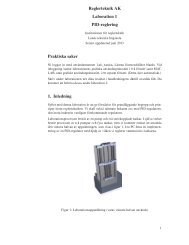
Figure 2.1 Coupling <strong>of</strong> thermodynamic control volume <strong>and</strong> piston<br />
EXAMPLE 1—INITIAL CONDITIONS<br />
Consider the simple system <strong>of</strong> a gas filled control volume in contact with<br />
a heat reservoir, Figure 2.1, closed by a piston held by a spring. Assuming<br />
that the cylinder is tightly closed, the equations for the control volume<br />
25
Chapter 2. Modeling Techniques<br />
are:<br />
pV = MasRT → pV = const T<br />
dT<br />
Mascv<br />
dt =−pdV + q<br />
dt<br />
V = V0 + Ax<br />
For the control volume by itself, two initial conditions have to be specified,<br />
typically pressure <strong>and</strong> temperature.<br />
The force balance on the piston gives<br />
mpiston<br />
d2x = kx − pA<br />
dt2 where k is the spring constant <strong>and</strong> A is the piston area. The piston as a<br />
st<strong>and</strong>-alone model needs two initial conditions, position <strong>and</strong> speed. When<br />
the system is combined, it is no longer possible to specify four independent<br />
initial conditions. With given piston position <strong>and</strong> speed, only the<br />
temperature or the pressure can be specified.<br />
When the gas volume is used for the initial condition <strong>of</strong> the control<br />
volume, it is obvious that the volume <strong>and</strong> piston position have to be consistent.<br />
While this example is trivial, finding consistent initial conditions<br />
for more complex high index DAE is difficult. Simulation tools for areas<br />
where high index problems are common provide algorithmic aid for finding<br />
consistent initial conditions.<br />
Definition: Equation 2.7 has differential index di = m if m is the<br />
minimal number <strong>of</strong> analytic differentiations<br />
F(x, ˙x, y, t) =0,<br />
df(x, ˙x, y)<br />
dt<br />
= 0, ...,<br />
d m f(x, ˙x,y)<br />
dt m = 0 (2.11a)<br />
such that equations 2.11 can be transformed by algebraic manipulations<br />
into an explicit ordinary differential system ˙x = Φ(x, u) which is called<br />
the “underlying ODE”.<br />
Two practical problems arise with the numerical solution <strong>of</strong> DAE:<br />
• calculation <strong>of</strong> consistent initial conditions <strong>and</strong><br />
• reliable numerical solution <strong>of</strong> the trajectories.<br />
The details <strong>of</strong> the difficulties <strong>of</strong> the numerical solution are described in<br />
[Hairer <strong>and</strong> Wanner, 1996]. A few solution methods for DAE are actually<br />
capable <strong>of</strong> h<strong>and</strong>ling high index DAE directly. Another possibility is to use<br />
26
2.1 Representation <strong>of</strong> Dynamics<br />
the definition (2.11) as a symbolic procedure to reduce a DAE to index 1.<br />
This option <strong>of</strong>fers more <strong>and</strong> particularly more reliable possibilities for the<br />
numerical solution.<br />
If high index DAE would be a rare exception, they would not deserve<br />
much attention. They are very common, especially when systems are modeled<br />
by dividing them into subsystems, the key property <strong>of</strong> object oriented<br />
model libraries. Because <strong>of</strong> this, libraries would be useless if the simulation<br />
environment could not deal with the index problem. Either the numerical<br />
solver has to deal with the index directly – this is limited to cases<br />
<strong>of</strong> index 2 or 3 – or the simulation tool has to do symbolic index reduction.<br />
Modelica is designed to allow symbolic index reduction. The Dymola 2 tool<br />
that was used in the development <strong>of</strong> the ThermoFluid library does a good<br />
job at detecting <strong>and</strong> (most <strong>of</strong>ten) reduce higher index to index one which<br />
Dymola can integrate, but nonetheless it is valuable to know when <strong>and</strong><br />
why high index DAE will occur. The most typical occurrences are:<br />
Simplification: imposing constraints between states (or quantities related<br />
to them) due to a simplifying assumption introduces an index<br />
problem. In process engineering these constraints are <strong>of</strong>ten in the<br />
form <strong>of</strong> “unmodeled” flows, e.g. mass flows which are not calculated<br />
explicitly. St<strong>and</strong>ard cases are<br />
• Incompressibility volume constraint<br />
• Phase equilibrium constrained sum <strong>of</strong> volumes.<br />
• Reaction equilibrium fixed ratio between concentrations <strong>of</strong><br />
components.<br />
Coupling: high index due to coupling <strong>of</strong> models is a special case <strong>of</strong> simplification<br />
because it arises from idealized couplings, e. g., connecting<br />
two capacitors in parallel. The simplification is to assume that<br />
the resistance between them really is zero. In this case the current<br />
between the capacitors is the unmodeled flow. High index due to<br />
coupling is the most important reason why object-oriented modeling<br />
requires automatic h<strong>and</strong>ling <strong>of</strong> high index problems.<br />
Perfect control: Specifying the trajectory <strong>of</strong> an output variable as a time<br />
function imposes a trajectory constraint on the states <strong>and</strong> thus also<br />
leads to an index problem.<br />
The problem <strong>of</strong> high index models is usually discussed in detail in<br />
all modeling courses for process engineering, see [Pantelides, 2000] <strong>and</strong><br />
[Preisig, 2001]. The following example demonstrates that high index problems<br />
are <strong>of</strong>ten introduced through simplifying assumptions. While this is<br />
2Dymola is a simulation environment using the Modelica language by the Swedish company<br />
Dynasim AB.<br />
27
Chapter 2. Modeling Techniques<br />
˙m ev<br />
j−1<br />
˙vj−1<br />
˙m ev<br />
j<br />
m j = ρ j Vj<br />
msj = cjVj<br />
˙vj<br />
Figure 2.2 Series <strong>of</strong> salt basins<br />
˙m ev<br />
j+1<br />
typical <strong>and</strong> well-known for mechanical <strong>and</strong> electrical systems, this example<br />
shows a simple process model <strong>of</strong> open evaporation basins for salt<br />
harvesting. The example is a variation <strong>of</strong> an example from [Weiss <strong>and</strong><br />
Preisig, 2000]<br />
EXAMPLE 2—SALT BASINS IN SERIES<br />
Consider a series <strong>of</strong> salt basins as in Figure 2.2. At the top <strong>of</strong> each basin<br />
are inflows <strong>of</strong> low concentration salt brine. Water evaporates in each basin<br />
<strong>and</strong> the outflow into the next lower basin has a higher salt concentration.<br />
It is difficult to model the exact flow into the next basin 3 , but an adequate<br />
simplification is to assume that the brine volume equals the maximum<br />
value <strong>of</strong> the basins volume. The brine in the j-th basin is assumed to have<br />
a density that depends on the salt concentration cj. The model for each<br />
basin j, j ∈ 2..N can be written as follows:<br />
˙m j = ρ j−1 ˙vj−1 − ˙m ev<br />
j − ρ j ˙vj total mass balance (2.12a)<br />
˙msj = cj−1 ˙vj−1 − cj ˙vj<br />
salt mass balance (2.12b)<br />
mj = ρ j Vj mass m (2.12c)<br />
msj = cjVj<br />
salt mass ms (2.12d)<br />
xsj = mj<br />
msj<br />
salt concentration xs (2.12e)<br />
ρ j =(xsj) function to calculate density ρ (2.12f)<br />
The inflow conditions into the first basin, c0 <strong>and</strong> ˙v0, are known. For<br />
a known evaporation mass flow rate ˙m ev<br />
j this is a well-posed index two<br />
DAE problem. For each basin, there are 6 variables: m, ms, ˙v, xs, ρ <strong>and</strong><br />
c (V, ˙m ev are assumed known), as well as 6 equations. But there are<br />
28<br />
3 The overflows in open air salt basins have irregular geometries.
2.1 Representation <strong>of</strong> Dynamics<br />
no explicit equations for ˙v, these have to be calculated from the volume<br />
constraint <strong>and</strong> the mass balances. By differenting the volume constraint,<br />
the concentration equation <strong>and</strong> the density definition, it is possible to<br />
compute the volumetric flow explicitly:<br />
˙vj = ′ (xsj)(xsj − xsj−1)ρj−1 + ρj−1ρj<br />
ρ 2 j−1<br />
˙vj−1 + ′ (xsj)xsj + ρj−1<br />
ρ 2 j−1<br />
Modelica was designed to make algorithmic approaches to these transformations<br />
possible. The algorithmic conversion to an index one problem<br />
involves detecting the constraint equations <strong>and</strong> differentiating them symbolically.<br />
Two algorithms provide the necessary methods: Pantelides’ algorithm<br />
[Pantelides, 1988] <strong>and</strong> the method <strong>of</strong> Dummy-Derivatives [Mattsson<br />
<strong>and</strong> Söderlind, 1993]. A remaining problem is to select which <strong>of</strong> the<br />
differentiated variables is going to be used by the numerical integrator.<br />
Clearly, the index two DAE with the implicit definition <strong>of</strong> the volume<br />
flow is much easier to derive than the equation which is the result <strong>of</strong><br />
transforming the problem to an index one problem. The algebraic constraint<br />
is caused by the constant volume assumption. Equations 2.12c,<br />
2.12e <strong>and</strong> 2.12f have to be differentiated, then it is possible to calculate<br />
˙vj explicitly <strong>and</strong> reduce the problem to index one.<br />
There are three points to note in the index reduction procedure used<br />
above:<br />
• In spite <strong>of</strong> two differential equations there is only one independent<br />
state per basin.<br />
• Index reduction involves a global analysis <strong>of</strong> the equations, the volumetric<br />
flow ˙vj contains variables from the upstream basin.<br />
• The algorithmic solution <strong>and</strong> manual index reduction yield the same<br />
solution.<br />
With object-oriented modeling <strong>of</strong> each basin <strong>and</strong> local index reduction by<br />
the modeler this would mean that the concentration xsj <strong>of</strong> the upstream<br />
basin would have to be in the connectors, which is not obvious from the<br />
original equations. Similar problems occur in boiler modeling, see [Åström<br />
<strong>and</strong> Bell, 2000].<br />
In some engineering domains the presence <strong>of</strong> a high index DAE is<br />
regarded as a modeling error, which may actually be true. In other domains<br />
(electrical <strong>and</strong> mechanical) high index problems occur naturally<br />
from st<strong>and</strong>ard modeling assumptions. These differences lead to drastically<br />
different ways <strong>of</strong> dealing with the index problem:<br />
˙mj<br />
29
Chapter 2. Modeling Techniques<br />
• Send the modeler back to the step 1 to resolve the problem with<br />
pen <strong>and</strong> paper, reformulating the model into an equivalent index 1<br />
problem.<br />
• Build the capacity <strong>of</strong> recognizing <strong>and</strong> resolving high index problems<br />
into the modeling tool.<br />
Because Modelica is designed as a multi-domain modeling tool, it has to<br />
support automatic index h<strong>and</strong>ling. This does not mean that automatic<br />
index reduction is the silver bullet that solves all high index problems in<br />
the best possible way. There are a few exceptions when manual derivation<br />
<strong>of</strong> an index 1 problem is preferable to the automatic procedure. This<br />
is the case when the automatic procedure gives results with numerical<br />
disadvantages, at least with the current version <strong>of</strong> the Modelica language<br />
<strong>and</strong> the index reduction algorithms in the Dymola tool. Examples <strong>of</strong> these<br />
rare cases are presented in Chapter 4. But independent <strong>of</strong> an automatic<br />
h<strong>and</strong>ling, model users have to underst<strong>and</strong> the implications <strong>of</strong> high index<br />
problems in order to provide the right initial conditions.<br />
Partial Differential Equations<br />
Partial differential equations (PDE) are the mathematical formulations<br />
that permits the highest level <strong>of</strong> detail for system level models. They<br />
provide the tool corresponding to the magnifying glass with the highest<br />
magnification power. PDEs form an essential part <strong>of</strong> the mathematical<br />
description <strong>of</strong> physical systems depending on space <strong>and</strong> time. They arise<br />
in a large number <strong>of</strong> modeling applications, but are not that common in<br />
systems level modeling. The reason for this is that PDE can have widely<br />
differing properties <strong>and</strong> that they are much more difficult to deal with<br />
numerically than ODEs. Using PDE for dynamical systems means that<br />
we have at least one more independent variable apart from time. Usually<br />
these are spatial coordinates, but variables can also be distributed in other<br />
dimensions like particle sizes in crystallization processes.<br />
Numerical solutions to PDE for design calculations are used in almost<br />
all engineering disciplines <strong>and</strong> are established as independent research<br />
areas, e. g., Computational Fluid Dynamics (CFD) <strong>and</strong> Finite Element<br />
Methods (FEM).<br />
Consider a set <strong>of</strong> PDEs expressed over the solution domain Ω which is<br />
a compact region in IR m+1 <strong>and</strong> its boundary δ Ω ∈ IR m , compare Figure 2.3<br />
for a two-dimensional example. If the independent variables are separated<br />
into time t <strong>and</strong> a vector <strong>of</strong> spatial variables x, then the dependent variables<br />
u can be written as<br />
u = u(x, t)<br />
where u ∈ IR n , x ∈ IR m <strong>and</strong> t ∈ IR ≥ 0. In mathematical texts the independent<br />
space <strong>and</strong> time variables are usually treated alike, here Ω is used<br />
30
.<br />
n<br />
s<br />
Solution Domain: Ω<br />
:<br />
2.1 Representation <strong>of</strong> Dynamics<br />
Boundary: δ Ω<br />
Figure 2.3 Computational domain Ω <strong>of</strong> a PDE<br />
for the union <strong>of</strong> the spatial dimensions <strong>and</strong> time. The partial derivatives<br />
are <strong>of</strong>ten denoted as follows<br />
(ux)ij = ui<br />
, (uxx)ijk =<br />
xj<br />
2ui xjxk<br />
, etc.<br />
For modeling <strong>of</strong> physical systems, PDEs <strong>of</strong> second order account for<br />
many important applications. For simplicity <strong>of</strong> exposition we restrict the<br />
following discussion (adapted from [Logan, 1994]) to one space dimension<br />
x, a single scalar variable u <strong>and</strong> get<br />
G(x, t, u, ux, ut, uxx,utt, uxt) =0 (2.13)<br />
where the independent variable x <strong>and</strong> t lie in some given domain Ω. By<br />
a solution to (2.13) we mean a twice continuously differentiable function<br />
u(x, t) defined on Ω which, when substituted into 2.13 reduces 2.13 to an<br />
identity on the domain Ω. These solutions are called classical or genuine.<br />
When the solutions are extended to include functions which are discontinuous<br />
or have discontinuous derivatives, such functions are called weak<br />
solutions. For one-dimensional PDEs the solution <strong>of</strong> 2.13 can be represented<br />
as a smooth surface in three-dimensional xtu-space lying over the<br />
domain Ω in the xt-plane, as shown in Figure 2.4.<br />
Boundary <strong>and</strong> Initial Conditions In ordinary differential equations<br />
solutions depend on arbitrary constants. Initial or boundary conditions<br />
fix the arbitrary constant <strong>and</strong> pick out a unique solution. The situation<br />
31
Chapter 2. Modeling Techniques<br />
Pressure [bar]<br />
0.0<br />
1.2<br />
1.1<br />
0.2<br />
0.4<br />
Length [m]<br />
0.6<br />
5<br />
0.8<br />
1.0<br />
10<br />
15<br />
Time [ms]<br />
Figure 2.4 Graphical representation <strong>of</strong> the solution to the pressure wave demo<br />
model from the ThermoFluid library. The model simulates a pipe whose back end at<br />
(x = 1) was instantaneously opened to a lower pressure a few milliseconds before<br />
this “snapshot” <strong>of</strong> spacetime was taken. It represents the space-time diagram <strong>of</strong> a<br />
pressure wave traveling back <strong>and</strong> forth in a one-dimensional pipe model. It clearly<br />
shows one characteristic <strong>of</strong> a hyperbolic PDE, the wave moving from the back end <strong>of</strong><br />
the pipe (x = 1) to the front, reflection at the front (x = 0) <strong>and</strong> traveling towards the<br />
back end again. The slope <strong>of</strong> the linear ridges between the x- <strong>and</strong>taxes correspond<br />
to the characteristics, u + c <strong>and</strong> u − c with u gas flow speed <strong>and</strong> c speed <strong>of</strong> sound.<br />
for PDE is similar. Imposing initial <strong>and</strong> boundary conditions selects one<br />
from the infinitely many solutions. These auxiliary conditions are usually<br />
suggested by the underlying physical problem or by the type <strong>of</strong> the PDE.<br />
Conditions on u or its derivatives at t = 0 along segments <strong>of</strong> the domain<br />
boundary are called initial conditions while conditions along any other<br />
curves <strong>of</strong> the xt-plane are called boundary conditions. For a well-posed<br />
physical problem, a complete set <strong>of</strong> initial conditions has to be specified,<br />
i. e. u(x, t = 0) has to be known for all <strong>of</strong> Ω.<br />
A typical modeling error in PDE problems is to specify non-physical<br />
boundary conditions which lead to an ill-posed problem. For example, in<br />
heat - or electrical problems, a potential (temperature or voltage) hastobe<br />
specified somewhere on the boundary, otherwise the level <strong>of</strong> the potential<br />
is free to float <strong>and</strong> any potential level would give a mathematical solution.<br />
The mathematical literature traditionally classifies boundary condi-<br />
32<br />
20
2.1 Representation <strong>of</strong> Dynamics<br />
tions into three categories:<br />
• Dirichlet boundary conditions: u =on δ Ω<br />
• Neumann boundary conditions: u<br />
u<br />
n =or s =on δ Ω<br />
• Robin boundary conditions: u<br />
+ ku =,k>0onδΩ<br />
n<br />
Here n denotes an outward normal vector <strong>and</strong> s a tangential vector<br />
with respect to the boundary δ Ω at a given point, see Figure 2.3. Dirichlet<br />
boundary conditions can be applied exactly on δ Ω when is analytic, but<br />
practical problems with Neumann <strong>and</strong> Robin conditions are that errors<br />
are easily introduced when representing them numerically.<br />
In some interesting problems the calculation <strong>of</strong> the boundary location<br />
is part <strong>of</strong> the problem <strong>and</strong> not known in advance. Moving boundary<br />
problems are associated with time dependent processes where behavior<br />
changes abruptly at a boundary which changes its location in space. Flame<br />
propagation <strong>and</strong> phase change problems are typical examples <strong>of</strong> moving<br />
boundary problems.<br />
Symbolic approaches to the solution <strong>of</strong> PDE <strong>of</strong>ten involve free functions<br />
<strong>of</strong> a certain type which have to fulfill the boundary conditions. Fourier’s<br />
approach <strong>of</strong> solving the heat conduction problem was to construct the<br />
solution as an infinite sum <strong>of</strong> functions all <strong>of</strong> which fulfill the homogeneous<br />
boundary conditions.<br />
Classification For second order PDEs, a special classification has been<br />
established both from a mathematical st<strong>and</strong>point <strong>and</strong> based on the physical<br />
phenomena that they arise from. From the physical point <strong>of</strong> view,<br />
there are three types <strong>of</strong> equations: those that govern diffusion processes,<br />
those that govern wave propagation <strong>and</strong> those that govern equilibrium<br />
phenomena. Equations <strong>of</strong> mixed type also occur, but locally for a fixed<br />
point ω ∈ Ω they belong to one <strong>of</strong> the three categories. Considering a<br />
single, second order PDE <strong>of</strong> the form<br />
auxx + 2buxt + cutt = d(x, t, u, ux, ut), (x, t) ∈Ω (2.14)<br />
where a, b <strong>and</strong> c are continuous functions on Ω <strong>and</strong> not all <strong>of</strong> a, b <strong>and</strong><br />
c vanish simultaneously at some point <strong>of</strong> Ω. Also the function d on the<br />
right h<strong>and</strong> side is assumed to be continuous. The equation is classified on<br />
the basis <strong>of</strong> its second order derivatives using the discriminant Δ, defined<br />
by Δ = b 2 − ac. Then (2.14) is said to be<br />
hyperbolic if Δ > 0, a wave propagation equation,<br />
parabolic if Δ = 0, a diffusion process equation or<br />
elliptic if Δ < 0, an equilibrium or steady-state process.<br />
33
Chapter 2. Modeling Techniques<br />
In the case <strong>of</strong> elliptic PDE, time derivatives do not occur <strong>and</strong> only space<br />
coordinates are independent variables. They are a rare exception in dynamical<br />
systems modeling. It should be pointed out again that the type<br />
<strong>of</strong> the equation may change on Ω because Δ depends on x <strong>and</strong> t.<br />
Numerical Methods for PDE The numerical solution <strong>of</strong> PDE is generally<br />
a difficult problem. Solutions are always approximations to the true<br />
mathematical solution <strong>of</strong> the equation <strong>and</strong> all the more to the real physics<br />
that they represent. Solutions can be very sensitive to small changes in<br />
parameters or boundary conditions. The situation is not hopeless, there<br />
are several numerical methods which can solve technically relevant problems<br />
reliably. There is active research in the area <strong>of</strong> solutions to PDE <strong>and</strong><br />
from the many methods available only the key features <strong>of</strong> a few <strong>of</strong> them<br />
will be discussed.<br />
A generalized concept that comprises the majority <strong>of</strong> numerical PDE<br />
solution methods is the “Method <strong>of</strong> Lines”. The methods <strong>of</strong> lines converts<br />
time dependent PDEs into ODEs (or DAEs) with respect to time<br />
by choosing a fixed spatial discretization <strong>and</strong> usually also a fixed order<br />
approximation to the spatial derivatives <strong>of</strong> u(x, t). The name “Method <strong>of</strong><br />
Lines” is based on the fact that many <strong>of</strong> these methods approximate the<br />
solution <strong>of</strong> the equations on a fixed spatial grid <strong>of</strong> straight lines. Method<br />
<strong>of</strong> lines as a group name also refers to finite element methods where the<br />
spatial discretization is fixed, but the discretization uses triangles <strong>of</strong> different<br />
sizes. Traditional PDE solvers also use a fixed time discretization,<br />
but in recent years it has become common to use variable time step ODE<br />
solvers for discretized PDE.<br />
The method <strong>of</strong> lines can provide good numerical approximations to the<br />
solution <strong>of</strong> PDE in a wide variety <strong>of</strong> applications. The family <strong>of</strong> methods<br />
<strong>of</strong> lines comprises finite difference, finite volume, finite element <strong>and</strong><br />
weighted residual methods in which piecewise local or global approximation<br />
functions in the space dimension are used to convert hyperbolic<br />
<strong>and</strong> parabolic PDE problems into initial value ODE problems. The key<br />
advantage <strong>of</strong> the “Method <strong>of</strong> Lines” is tw<strong>of</strong>old:<br />
• It is straightforward to combine subsystem models which are described<br />
by DAEs or ODEs with PDEs because they are all converted<br />
to the same mathematical form.<br />
• ODE <strong>and</strong> DAE solvers can be employed for the solution. These<br />
solvers have reached a higher degree <strong>of</strong> sophistication than PDE<br />
solvers. Many programs are available which permit fast <strong>and</strong> accurate<br />
solutions to large sets <strong>of</strong> DAE [Petzold, 1982].<br />
The advantage <strong>of</strong> ODE/DAE solvers is that they use sophisticated algorithms<br />
to adjust the time step size <strong>and</strong> the order <strong>of</strong> a method in order to<br />
34
2.1 Representation <strong>of</strong> Dynamics<br />
control the user-specified approximation error [Gustafsson, 1992].<br />
However, the advantage <strong>of</strong> the method points to the disadvantage: The<br />
DAE solver used for integration in time cannot control or even estimate<br />
the space discretization error. For coarse discretizations the spatial error<br />
can easily be an order <strong>of</strong> magnitude larger than the (controlled) time discretization<br />
error. There are no general guidelines on how to determine<br />
the spatial discretization such that a computationally efficient <strong>and</strong> accurate<br />
solution is obtained. Trial <strong>and</strong> error <strong>and</strong> engineering intuition are<br />
the prevailing methods. Adaptive or moving grid methods are attempts<br />
to h<strong>and</strong>le the spatial discretization error better, but their complexity <strong>and</strong><br />
restriction to special classes <strong>of</strong> problems has discouraged implementation<br />
in general purpose simulation tools [Oh, 1995]. This is one <strong>of</strong> the problems<br />
in using PDE in systems modeling: there are many special methods for<br />
special cases, which makes implementation <strong>of</strong> general purpose tools for<br />
all types <strong>of</strong> PDE prohibitively complex.<br />
Discrete Time <strong>and</strong> Hybrid Systems<br />
Discrete time dynamic systems arise from the time discretization <strong>of</strong> continuous<br />
systems or from time scale abstractions <strong>of</strong> such systems. In physical<br />
systems modeling they are the predominant way to model control<br />
actions <strong>of</strong> all kind: finite difference equations <strong>and</strong> discrete time transfer<br />
functions for feedback control <strong>and</strong> particular description formalisms<br />
such as Petri nets, [Murata, 1989; David <strong>and</strong> Alla, 1992], finite state machines,<br />
[Kohavi, 1978], Grafcet, [Årzén, 1994; Johnsson <strong>and</strong> Årzén, 1999],<br />
Grafchart [Årzén, 1996; Johnsson, 1999] or State Charts [Harel, 1987]<br />
for sequential control, safety <strong>and</strong> redundancy management control logic.<br />
Changes <strong>of</strong> the state <strong>of</strong> discrete time systems occur only at discrete points<br />
in time.<br />
Most controllers are implemented as digital controllers with algorithms<br />
based on discrete time process models. The controllers <strong>of</strong>ten contain process<br />
models, e. g., in the form <strong>of</strong> Kalman filters. A discrete time model<br />
can be obtained by sampling the continuous time model. Sampling the<br />
continuous time ODE-model<br />
˙x(t) =Ax(t)+Bu(t), y(t)=Cx(t)<br />
at equidistant time instants with sampling interval h results in the discrete<br />
time model<br />
x(kh + h) =Φx(kh)+Γ(kh), y(kh) =Cx(kh)<br />
where Φ = e AH <strong>and</strong> Γ = h<br />
0 eAs Bds. There are also approximative discretization<br />
methods, including Euler’s method <strong>and</strong> Tustin’s approxima-<br />
35
Chapter 2. Modeling Techniques<br />
tion. Numerical methods for solving ODEs are mostly based on more sophisticated<br />
discrete approximations. Further details on discretization <strong>of</strong><br />
continuous time models can be found in [Åström <strong>and</strong> Wittenmark, 1990].<br />
Hybrid systems combine the continuous behavior specified by differential<br />
equations with discontinuous changes specified by discrete event<br />
switching logic or finite difference equations at sample times. For successful<br />
modeling <strong>of</strong> hybrid phenomena, the semantics <strong>of</strong> the hybrid modeling<br />
language elements have to be well understood. In certain difficult cases<br />
even an underst<strong>and</strong>ing <strong>of</strong> the implementation <strong>of</strong> the computational solution<br />
procedure are necessary. At least three modeling situations lead to<br />
hybrid phenomena in systems modeling:<br />
• Combination <strong>of</strong> continuous physical systems with discrete time, computer<br />
implemented control logic.<br />
• Discrete approximations to physical phenomena which exhibit steep<br />
changes within short time- or length scales, e. g., the time scale abstractions<br />
mentioned in Section 1.3 like colliding objects in mechanics.<br />
• The modeled device changes its characteristic behavior in the interesting<br />
range <strong>of</strong> operation so much that different states or even a<br />
different number <strong>of</strong> states are needed for an adequate description<br />
<strong>of</strong> the behavior. An example could be an evaporator that is flooded<br />
with liquid at startup.<br />
Modeling on a macroscopic scale <strong>of</strong>ten gives rise to empirical relations<br />
that are piecewise functions. Typical examples are friction, pressure drop<br />
or heat transfer correlations. As long as the relations do not change the<br />
causality <strong>of</strong> the calculation, these are fairly easy to h<strong>and</strong>le in simulation.<br />
Hybrid phenomena are still the topic <strong>of</strong> intensive research activity, even<br />
fundamental issues such as the existence <strong>and</strong> uniqueness <strong>of</strong> executions<br />
<strong>of</strong> hybrid automata are not understood in all details. Good introductions<br />
to ongoing research in hybrid systems is found in [Johansson et al., 1999]<br />
<strong>and</strong> [Zhang et al., 2000].<br />
From the point <strong>of</strong> view <strong>of</strong> numerical mathematics, the following classification<br />
can be made:<br />
36<br />
1. ODE or index 1 DAE where a discrete event or discontinuous function<br />
does not change the index or the size <strong>of</strong> the state vector.<br />
(a) Only the right h<strong>and</strong> side <strong>of</strong> the ODE/DAE changes discontinuously,<br />
all states are C 0 continuous. The values <strong>of</strong> the states<br />
before <strong>and</strong> after the event are the same. Computational causality<br />
<strong>of</strong> algebraic variables in an index 1 DAE might change also.
2.1 Representation <strong>of</strong> Dynamics<br />
(b) The states may change discontinuously through an impulsive<br />
action. Physically, this arises from a time scale abstraction. The<br />
mathematical tool is a Dirac impulse the amplitude <strong>of</strong> which<br />
has to be calculated. The values <strong>of</strong> the states after the event<br />
have to be calculated by conditions or extra equations in the<br />
model.<br />
2. ODE or DAE <strong>of</strong> any index where the index or the number <strong>of</strong> states<br />
changes after an event. Both <strong>of</strong> these change the dimension <strong>and</strong><br />
possibly the structure <strong>of</strong> the dynamical problem.<br />
(a) States are added to the state vector. From an implementation<br />
point <strong>of</strong> view the problem is similar to 1(b) because the new<br />
state needs to be initialized. Algebraic variables may also be<br />
added but this is less problematic.<br />
(b) Constraints on states are introduced during integration <strong>and</strong><br />
the index <strong>of</strong> the DAE changes. Causality might change <strong>and</strong><br />
a physically reasonable treatment <strong>of</strong> the problem may include<br />
Dirac impulses.<br />
In practical terms, the cases 1 are easier to h<strong>and</strong>le than the cases 2,<br />
modeling <strong>of</strong> them needs both support from the modeling language <strong>and</strong><br />
numerical solvers.<br />
The possibility that a system <strong>of</strong> equations may become singular during<br />
integration due to topological constraints is a related problem. This<br />
occurs for the pendulum in Cartesian coordinates [Mattsson et al., 2000]<br />
such that a different set <strong>of</strong> equations has to be used instead. Strictly<br />
speaking this is not a hybrid problem – the system’s numerical condition<br />
gets gradually worse – but the implementation problems are related.<br />
Many hybrid problems can usually be dealt with in an algorithmic<br />
fashion, but the challenge for a modeling language is to describe hybrid<br />
phenomena in an intuitive <strong>and</strong> completely declarative way. This is a complex<br />
task which is partially taken into account in Modelica although it<br />
does not yet <strong>of</strong>fer satisfactory solutions for the more difficult cases above.<br />
The first step in describing hybrid problems in a declarative manner<br />
is to write equations in a way that allows the tool to automatically detect<br />
<strong>and</strong> locate the time <strong>of</strong> events. This is done with the help <strong>of</strong> indicator<br />
or crossing functions (see [Cellier, 1991]) which change their sign at the<br />
discontinuity. In Modelica, these crossing functions are automatically generated<br />
from the declarative discontinuity conditions. Users only have to<br />
supply their own crossing functions when the discontinuities are hidden,<br />
e. g., in external programming code.<br />
A particularly annoying problem for practitioners is the phenomenon<br />
<strong>of</strong> “chattering” which occurs sometimes in case 1a above. It is an unwanted<br />
37
Chapter 2. Modeling Techniques<br />
ε<br />
Figure 2.5 Chattering (ε not to scale)<br />
effect which under certain circumstances is triggered by the exact event<br />
location. On the other h<strong>and</strong>, the exact event location is a precondition to<br />
high accuracy solution <strong>of</strong> the system trajectory. A zoom into the solution<br />
trajectory in the case <strong>of</strong> chattering is given in Figure 2.5. Two different<br />
right-h<strong>and</strong> sides <strong>of</strong> the ODE are symbolized by the two vector fields. In<br />
this case both vector fields give a gradient that drives the solution towards<br />
the discontinuity. The solver locates the exact time point on the trajectory<br />
when the discontinuity triggers <strong>and</strong> restarts the solver with the new right<br />
h<strong>and</strong> side. Note that omitting the step <strong>of</strong> locating the discontinuity exactly<br />
leads a large error in the solution trajectory because the wrong vector field<br />
is used for a large part <strong>of</strong> the time step. The restart is computationally<br />
expensive, multi-step high order methods restart with low order <strong>and</strong> small<br />
step size. In order to account for small numerical errors, the solver will<br />
not switch back to the old right h<strong>and</strong> side within a small ε -environment<br />
around the discontinuity. The gradient will drive the trajectory across<br />
the discontinuity again <strong>and</strong> this repeats for many times. The progress in<br />
simulation gets prohibitively slow <strong>and</strong> this is experienced as a st<strong>and</strong>-still<br />
in simulation.<br />
Currently there is no simulation tool which treats the chattering problem<br />
in a satisfying way or would even give a clear diagnosis <strong>of</strong> the occurrence.<br />
The pragmatic solution as <strong>of</strong> today is to change the hybrid model to<br />
a smooth, continuous model, compare Figure 2.6. Physically this is <strong>of</strong>ten<br />
an admissible solution because <strong>of</strong>ten the hybrid phenomenon is a result<br />
<strong>of</strong> an abstraction that can equally well be parameterized in a smooth way.<br />
The change in Reynolds number between laminar <strong>and</strong> turbulent flow is<br />
such a case as well as boundary layers in temperature or velocity fields.<br />
38
2.2 Model Libraries<br />
For certain classes <strong>of</strong> hybrid systems <strong>and</strong> for this type <strong>of</strong> chattering or<br />
“sliding mode” behavior, efficient <strong>and</strong> accurate simulation methods were<br />
explored in [Malmborg, 1998] <strong>and</strong> [Mattsson, 1996] using the concept <strong>of</strong><br />
Filippov solutions. However, these methods are not general <strong>and</strong> not implemented<br />
in simulation packages yet.<br />
Area with smoothened behaviour<br />
Figure 2.6 Chattering is avoided by smoothing the discontinuity. The Filippov<br />
solution can be visualized by letting the gray area shrink to zero width. The sum <strong>of</strong><br />
the vector fields defines the gradient on the boundary.<br />
From a modeling perspective it is very natural to combine DAE descriptions<br />
with hybrid phenomena. This leads to many interesting problems<br />
such as DAEs which change their index when a discrete submodel<br />
switches states. There are many interesting research problems stimulated<br />
by such models: some semantic issues related to declarative descriptions<br />
<strong>and</strong> reliable execution <strong>of</strong> simulation <strong>of</strong> the models are still open problems.<br />
2.2 Model Libraries<br />
Model libraries are collections <strong>of</strong> reusable model parts <strong>and</strong> subsystems in<br />
a modeling <strong>and</strong> simulation tool. In object-oriented modeling these parts<br />
will almost always coincide with physical model parts <strong>and</strong> subsystems.<br />
Model libraries can increase reusability <strong>and</strong> consequently productivity in<br />
systems modeling substantially. This has been one <strong>of</strong> the main incentives<br />
in the development <strong>of</strong> object-oriented model libraries during the last two<br />
39
Chapter 2. Modeling Techniques<br />
decades. In the following discussion we will restrict the subject to physics<br />
based models for engineering systems.<br />
Classification<br />
Model libraries in some form are part <strong>of</strong> all modern simulation tools. On<br />
the first look, they seem to follow the same ideas: model components can<br />
be dragged from a model palette or browser onto a diagram which is used<br />
to compose a complex system from simpler parts. In terms <strong>of</strong> their implementation<br />
<strong>and</strong> usefulness for different purposes, there can be tremendous<br />
differences. Most domain specific modeling tools do not show the details<br />
<strong>of</strong> the model implementation <strong>and</strong> a user has to rely on the completeness<br />
<strong>and</strong> correctness <strong>of</strong> the documentation. These black box models, even if<br />
they are based on sound physical models, can only serve some simulation<br />
purposes. However, other tasks such as model validation is much more<br />
difficult or even impossible. Internally, different models may be used for<br />
different ranges <strong>of</strong> parameters or operating conditions. This is for example<br />
the case for the SPICE [Massobrio <strong>and</strong> Antognietti, 1993], but at least the<br />
source code for the SPICE models is available even if sparse documentation<br />
may make it difficult to comprehend. Trusting black box models can<br />
be a hazard. K. J. Åström has described this in the following way:<br />
The practice <strong>of</strong> not publishing source code is a factor which<br />
strongly contributes to poor quality (<strong>of</strong> models). A good analogy<br />
is to ask the question: what would mathematics look like if<br />
theorems were published together with a manual how to use<br />
them <strong>and</strong> the pro<strong>of</strong>s were hidden as company secrets?<br />
The philosophy behind the Modelica language <strong>and</strong> other equation based<br />
modeling languages is orthogonal to black box models. Model users should<br />
be able to see all equations that comprise the model. They should also be<br />
allowed to modify <strong>and</strong> extend the model if necessary for them. Open Code<br />
libraries can be designed with different ideas about their use in mind. In<br />
some domains it is possible to provide a complete set <strong>of</strong> base models, e. g.,<br />
in the Modelica Multi-Body-Systems (MBS) library. This library is open<br />
<strong>and</strong> extensible. It was designed to be complete for all common MBS. In<br />
process engineering <strong>and</strong> thermodynamic systems it is impossible to provide<br />
a library <strong>of</strong> similar completeness as the MBS library because <strong>of</strong> a<br />
large number <strong>of</strong> model assumptions <strong>and</strong> case-specific empirical correlations<br />
which lead to a huge number <strong>of</strong> models. Therefore, the ThermoFluid<br />
library has been designed from the start to provide base models <strong>and</strong> structure<br />
to help rapid model development. It is necessarily incomplete, but it<br />
<strong>of</strong>fers hooks <strong>and</strong> st<strong>and</strong>ard-case placeholders for user written model extensions.<br />
Three types <strong>of</strong> libraries can be distinguished:<br />
40
2.2 Model Libraries<br />
Black Box model libraries This is the most widespread case for commercial<br />
domain specific libraries, e. g., in Adams [Adams, 2002],<br />
APROS [Juslin, 1995] <strong>and</strong> ITISIM [ITI GmbH, 2002].<br />
Open Code model libraries The Modelica St<strong>and</strong>ard Library is a typical<br />
open code library. The st<strong>and</strong>ard models are selected in a way<br />
that covers many common cases <strong>and</strong> defines connectors which are<br />
valid for all models in that domain.<br />
User Extensible Libraries The idea <strong>of</strong> a user extensible base library<br />
has been explored with the ThermoFluid library. That the concept<br />
works well for a broad range <strong>of</strong> processes which are only related<br />
through their basic physical phenomena will be clear from the examples<br />
in Chapter 5. User extensible libraries have to be open code<br />
libraries.<br />
The main topic <strong>of</strong> this thesis is user extensible model libraries. Modelica<br />
<strong>of</strong>fers many language constructs that make Modelica particularly<br />
interesting for this type <strong>of</strong> library development.<br />
Structuring, Interfaces <strong>and</strong> Decomposition<br />
With the simple guideline that model structuring <strong>and</strong> interfaces correspond<br />
to the equivalent features <strong>of</strong> the real system, structuring <strong>of</strong> model<br />
libraries should be trivial. This is not quite true for several reasons. As<br />
soon as hierarchical decomposition is used, the number <strong>of</strong> levels <strong>and</strong> the<br />
interfaces between subsystems are debatable. Many levels may give a<br />
completely logical structure but may be cumbersome to browse <strong>and</strong> use.<br />
Too fine-grained decomposition can result in a large number <strong>of</strong> models<br />
with good code reuse but it is difficult to get an overview. There are many<br />
possible solutions how the obvious physical quantities in the interface <strong>of</strong><br />
a real system e. g., the flange <strong>of</strong> a pipe, are mapped to a mathematical<br />
model. Structuring is more important when the size <strong>of</strong> the model libraries<br />
<strong>and</strong> the organization using them grows. For very large libraries, databaselike<br />
search capabilities are necessary, otherwise modelers might prefer to<br />
rewrite a model instead <strong>of</strong> finding an existing one. This has been recognized<br />
as a common occurrence in large companies with many, <strong>of</strong>ten poorly<br />
documented models, see [Je<strong>and</strong>el et al., 1996].<br />
Many solutions for structuring <strong>of</strong> model libraries exist <strong>and</strong> <strong>of</strong>ten the<br />
resulting structure reflects personal preferences <strong>of</strong> the library designer.<br />
The library structure is always a compromise. The developer should take<br />
the prospective users into consideration. If the users want to assemble<br />
systems from subsystems <strong>and</strong> get simulation results as quickly as possible,<br />
complete subsystems representing parts <strong>of</strong> the system which are as<br />
large as possible with few parameters will help them most efficiently.<br />
41
Chapter 2. Modeling Techniques<br />
Users which have to develop models by themselves <strong>and</strong> have to deal<br />
with rapidly changing prototypes under development benefit a lot from<br />
a much more fine-grained structure. They will also prefer a multi-layered<br />
approach which gives them access to all levels <strong>of</strong> model composition from<br />
basic physical phenomena to subsystems.<br />
A detailed investigation <strong>of</strong> structuring <strong>of</strong> object-oriented libraries will<br />
be given in Chapter 6.<br />
2.3 Validation <strong>and</strong> Verification<br />
Models are developed with the purpose <strong>of</strong> drawing conclusions about the<br />
real system, either by simulating them with inputs which resemble the<br />
inputs <strong>of</strong> the real system or by analyzing them. Consequently, the validity<br />
<strong>of</strong> the model is a very important question. The model must accurately describe<br />
the important physical phenomena <strong>of</strong> the real system in order to be<br />
<strong>of</strong> any use. Validation <strong>of</strong> models is a complicated task. The fundamental<br />
problem is that no model can perfectly capture all aspects <strong>of</strong> the real system,<br />
abstraction <strong>and</strong> simplification are the very nature <strong>of</strong> modeling. Thus<br />
model validation is always relative to the requirements <strong>of</strong> the model use.<br />
It is important to recognize that it is impossible to conclusively validate<br />
a model. According to [Popper, 1935], a theory can only be falsified i. e.<br />
proven wrong by experimental tests. By passing any number <strong>of</strong> tests, a<br />
model is only as yet unfalsified. The art <strong>of</strong> model validation is thus to<br />
design validation test cases for the model that make sure the model holds<br />
sufficiently well for the interesting aspects <strong>of</strong> the real system. The part<br />
<strong>of</strong> model validation that deals with adaptation <strong>of</strong> parameters to make the<br />
model <strong>and</strong> the real system match is <strong>of</strong>ten called model calibration.<br />
There are two important aspects to the validation <strong>of</strong> mathematical<br />
models in a computer implementation:<br />
1. Does the model as it is coded in a modeling language correspond<br />
to the mathematical model that it is supposed to represent? This is<br />
called verification or internal validation.<br />
2. Does the model correspond to the real system? This is called validation,<br />
sometimes with the additional attribute external.<br />
For models obtained by system identification, validation <strong>of</strong> the model<br />
structure <strong>and</strong> parameters are part <strong>of</strong> the st<strong>and</strong>ard procedures in model<br />
development. For linear models the repertoire <strong>of</strong> systematic validation<br />
methods is rich <strong>and</strong> well established. The quantitative bounds that characterize<br />
the quality <strong>of</strong> the model give practitioners a good indication about<br />
how much they can trust a model. On the other h<strong>and</strong>, system identification<br />
models are inherently limited by being linear.<br />
42
2.3 Validation <strong>and</strong> Verification<br />
When validating models, there are two questions that have to be put:<br />
• Is the chosen model structure adequate?<br />
• Are the parameters used in the model optimal in some sense when<br />
the model output is compared to measurements <strong>of</strong> the real system.<br />
In practical terms the questions can usually not be separated like above,<br />
usually parameters are optimized for different model structures <strong>and</strong> then<br />
the structures are compared with their best-fit parameters. It is obvious<br />
that the choice <strong>of</strong> the model structure sets limits to the achievable<br />
performance <strong>of</strong> the model, see [Eborn, 2001]. The most common criterion<br />
for selecting a model structure is Akaike’s Information Criterion (AIC).<br />
It was developed for linear models but can also be applied to nonlinear<br />
models.<br />
The practical problem with model validation for first principle physical<br />
models is that they are non-linear. The mathematics <strong>and</strong> stochastics<br />
<strong>of</strong> nonlinear models are much less developed than for linear systems. Parameter<br />
optimization for hybrid-DAE models results in a nonlinear mixedinteger<br />
optimization problem which may be very hard to solve. Therefore,<br />
model calibration for physical models usually involves h<strong>and</strong>-tuning <strong>of</strong> parameters<br />
based on trial <strong>and</strong> error or physical insight. Often model <strong>and</strong><br />
system output are compared for typical input signals like step responses.<br />
Because <strong>of</strong> the current lack <strong>of</strong> systematic methods, this can be a very<br />
time-consuming activity, but for high quality models there is little chance<br />
to avoid it. The physical parameters <strong>of</strong> the real system are <strong>of</strong>ten not<br />
known accurately <strong>and</strong> may be impossible to measure directly. The model<br />
is calibrated by h<strong>and</strong>-tuning such parameters, sometimes with the help<br />
<strong>of</strong> optimization methods.<br />
One <strong>of</strong> the few attempts that have been made to bridge this gap between<br />
system identification <strong>and</strong> physical modeling by developing methods<br />
<strong>and</strong> tools for gray-box identification i. e. estimation <strong>of</strong> parameters in<br />
physical models is MoCaVa <strong>and</strong> its predecessor IDKIT developed at KTH<br />
by Bohlin <strong>and</strong> coworkers, see [Bohlin, 1991; Bohlin, 1998].<br />
A prototype <strong>of</strong> an integration <strong>of</strong> the modeling tool OMOLA <strong>and</strong> the greybox<br />
identification tool IDKIT was used to select between different structures<br />
for a non-linear drum boiler model. [Åström <strong>and</strong> Bell, 2000] had<br />
developed a series <strong>of</strong> simple drum boiler models <strong>of</strong> second, third <strong>and</strong> forth<br />
order. The third <strong>and</strong> forth order models were compared in [Sørlie <strong>and</strong><br />
Eborn, 1997; Sørlie <strong>and</strong> Eborn, 1998]. The results demonstrate that systematic<br />
model calibration can give very good agreements between model<br />
<strong>and</strong> real system <strong>and</strong> that the integration <strong>of</strong> a modeling <strong>and</strong> identification<br />
tool accelerates the work flow. Nonetheless this has not become industrial<br />
practice, mainly due to the lack <strong>of</strong> easy-to-use, integrated tools.<br />
43
Chapter 2. Modeling Techniques<br />
It is obvious from the definition <strong>of</strong> library models <strong>and</strong> validation that<br />
external validation <strong>of</strong> library models is not possible because they do not<br />
represent any particular real system. The internal validation on the other<br />
h<strong>and</strong> is very important because users <strong>of</strong> the library rely on the internal<br />
validation when they select models. In practical terms internal validation<br />
for library models means that the implemented model corresponds to its<br />
documentation 4 . Automated regression tests <strong>and</strong> cross checking numerical<br />
results with analytic ones where these exist for special cases are tools that<br />
can be used to obtain a high quality internal validation <strong>of</strong> library models.<br />
2.4 Physics Based Model Reduction<br />
The main purpose <strong>of</strong> dynamic models is to capture the dynamic behavior <strong>of</strong><br />
a system. When the model is to be used for control, the dynamic accuracy<br />
<strong>of</strong> the model is important in the vicinity <strong>of</strong> the crossover frequency <strong>of</strong> the<br />
feedback loop <strong>and</strong> less important at other frequencies. When controllers<br />
with integral action are used, the closed loop gain is infinity at ω = 0<strong>and</strong><br />
therefore the accuracy <strong>of</strong> the open loop gain at ω = 0 is not important, neither<br />
are the properties at frequencies that are higher than the crossover<br />
frequency. As a motivating example, an investigation <strong>of</strong> a model reduction<br />
from the electrical domain will be presented as a general, but simple<br />
case <strong>of</strong> dynamic model reduction. Often the question arises whether it<br />
is possible to lump energy storage <strong>of</strong> two closely connected physical submodels<br />
into one unit or not. The Modelica language <strong>and</strong> in particular the<br />
Dymola simulation tool allow to design model libraries where the tedious<br />
part <strong>of</strong> such model reduction procedures is h<strong>and</strong>led automatically be the<br />
tool when the user chooses model combinations that call for this simplification.<br />
The details <strong>of</strong> how this works in thermo-hydraulic cases will be<br />
presented in the following.<br />
Example: An Electrical Circuit<br />
The example consists <strong>of</strong> the simple electric circuit in Figure 2.7. The<br />
source voltage is the input to the system, the voltage over the capacitor<br />
C2 is the output. The system can be transformed into a linear state<br />
space system with the voltages <strong>of</strong> the two capacitances as states. The<br />
4Note that it is well possible for a model to pass an external validation with respect to a<br />
real system <strong>and</strong> to fail the internal validation.<br />
44
V in<br />
R1<br />
R=1<br />
2.4 Physics Based Model Reduction<br />
R2<br />
R=1<br />
VS1 C1 C2<br />
C=2 C=1 Vout Ground<br />
Figure 2.7 Simple electrical circuit with two capacitors.<br />
linear system becomes:<br />
<br />
˙x = Ax + Bu<br />
x =<br />
y = Cx<br />
<br />
−<br />
A =<br />
R1+R2<br />
<br />
1<br />
C1C2R1 C1R2 , B =<br />
− 1<br />
C2R2<br />
− 1<br />
C2R2<br />
with the transfer function<br />
vC1<br />
vC2 <br />
1<br />
C1R1<br />
0<br />
<br />
<br />
, C = (0 1)<br />
1<br />
C1C2R1R2s 2 + s(R1(C1 + C2)+C2R2)+1 .<br />
vout<br />
=<br />
vin<br />
The system stores energy in the two capacitors. The question <strong>of</strong> interest<br />
is now: under which circumstances is it possible to describe the system<br />
with one capacitor <strong>of</strong> the capacitance C1 + C2 instead <strong>of</strong> two? A simple way<br />
to do the model reduction is to neglect the resistance <strong>and</strong> set R2 = 0. The<br />
transfer function simplifies to<br />
vout<br />
vin<br />
=<br />
1<br />
sR1(C1 + C2)+1 .<br />
This has the effect to lump the capacitors into one with the sum <strong>of</strong> the original<br />
capacitances. Observe that a second order linear ODE system where<br />
we simply set R2 = 0 is singular. In the DAE-framework this is easy to<br />
treat. From R2 = 0wehavethatvC1=vC2, the constraint equation, compare<br />
Section 2.1, <strong>of</strong> the index 2 DAE. The index reduction can be h<strong>and</strong>led<br />
automatically, resulting in a reduced order ODE system. The singularity<br />
45
Chapter 2. Modeling Techniques<br />
Magnitude <strong>of</strong> the Eigenvalues<br />
0<br />
2<br />
4<br />
6<br />
8<br />
10<br />
12<br />
Eigenvalues <strong>of</strong> the System as a Function <strong>of</strong> R2<br />
Lumped Eigenvalue<br />
Fast Eigenvalue<br />
SlowEigenvalue<br />
0 200 400 600 800 1000<br />
Resistance <strong>of</strong> R2<br />
Figure 2.8 Eigenvalues <strong>of</strong> dynamics matrix A for the electrical system in Figure<br />
2.7<br />
problem <strong>of</strong> the higher order ODE formulation is avoided. This feature <strong>of</strong><br />
the DAE formulation can also be exploited for model order reduction for a<br />
non-zero, but small R2. For a choice <strong>of</strong> parameters R1 = 1000, C1 = 0.002<br />
<strong>and</strong> C2 = 0.001 we look at the eigenvalues <strong>of</strong> A (Figure 2.8) <strong>and</strong> the Bode<br />
plot (Figure 2.9) <strong>of</strong> the transfer function as R2 decreases. As can be seen<br />
from Figure 2.8, one eigenvalue is around 1/3 whereas the other goes to<br />
infinity as R2 gets small. For comparison, the constant eigenvalue resulting<br />
from a simplified circuit with R2 = 0 <strong>and</strong> <strong>and</strong> a lumped capacitor with<br />
C = C1 + C2 is also shown. From the look at the eigenvalues it seems to be<br />
possible to neglect the resistance R2 for values <strong>of</strong> R2 < 500. Observe that<br />
the eigenvalues are independent <strong>of</strong> the choice <strong>of</strong> inputs <strong>and</strong> outputs. An<br />
inspection <strong>of</strong> the bode plot in Figure 2.9 for the chosen input- <strong>and</strong> output<br />
signals reveals that the justification <strong>of</strong> the model reduction depends on<br />
the frequency content <strong>of</strong> the input signal. It is clear from the bode plot<br />
that the closed loop b<strong>and</strong>width is the limiting factor that determines for<br />
which values <strong>of</strong> R2 it is possible to use the simplified system. It is clearly<br />
not advisable to neglect any <strong>of</strong> the energy stores C1 or C2 which are <strong>of</strong><br />
the same order <strong>of</strong> magnitude. After this short excursion into the electrical<br />
domain, a similar situation for thermodynamic models is explored.<br />
46
Phase (deg) Magnitude (dB)<br />
0<br />
−50<br />
−100<br />
−150<br />
0<br />
−45<br />
−90<br />
−135<br />
10 −2<br />
−180<br />
10 −1<br />
10 0<br />
2.4 Physics Based Model Reduction<br />
10 1<br />
Frequency (rad/sec)<br />
10 2<br />
10 3<br />
R2 = 500<br />
R2 = 50<br />
R2 = 0.0<br />
Figure 2.9 Bode Plots <strong>of</strong> the electrical system in Figure 2.7 for different values<br />
<strong>of</strong> R2<br />
Heat Exchangers<br />
The type <strong>of</strong> model reduction presented in the previous example seems<br />
natural in that case. When the example is transferred to heat exchangers<br />
instead, the equivalent model reduction is not commonly used. Exceptions<br />
are special purpose low order models like the drum boiler model by<br />
[Åström <strong>and</strong> Bell, 2000]. This model reduction refers to an interesting case<br />
from Section 4.10 <strong>of</strong> combining a solid structure with a fluid when both the<br />
boundary layer heat resistance <strong>and</strong> the metal resistance are neglected. Instead<br />
<strong>of</strong> having separate energy balances for the wall <strong>and</strong> the fluid, these<br />
are combined into one energy store, equivalent to the lumping <strong>of</strong> the capacitors<br />
in the last example. Equating the temperatures Tfluid1 =Tm (see<br />
Figure 4.6) gives the wanted result. Again, an index two DAE system is<br />
the result where Tfluid1 =Tm is the constraint equation which is used to<br />
calculate the heat flow when differentiated. This means, similarly as in<br />
the electrical case, that the heat flow resistance is set to zero. Assuming<br />
for now that the fluid uses pressure p <strong>and</strong> specific enthalpy h as states<br />
10 4<br />
47
Chapter 2. Modeling Techniques<br />
<strong>and</strong> that the thermodynamic equation <strong>of</strong> state is explicit in these states,<br />
the temperature difference can be expressed as<br />
<br />
<br />
dT T <br />
= <br />
dp T <br />
+ <br />
dh<br />
(2.15)<br />
dt p dt h dt<br />
in the one phase region <strong>and</strong> as<br />
dTsat<br />
dt<br />
h<br />
= dTsat<br />
dp<br />
dp<br />
dt<br />
p<br />
(2.16)<br />
in the two phase region, where the temperature does not depend on the<br />
enthalpy. Usually the temperature is calculated via a function <strong>and</strong> not<br />
an equation. In current Modelica implementations, functions can not be<br />
differentiated unless a derivative function is written by the user <strong>and</strong> the<br />
annotation for function derivatives (see Section 3.4) is used to convey<br />
the derivative information to the simulator. If this is implemented in the<br />
model library, the model reduction is automatic whenever a user connects<br />
a fluid control volume <strong>and</strong> a resistance-free wall model without an explicit<br />
heat transfer law between them. The validity <strong>of</strong> doing this model<br />
reduction depends on the parameters <strong>of</strong> the actual physical system: in a<br />
condenser with very high heat transfer coefficients this assumption is usually<br />
valid for the condensing flow. The same holds for most walls in contact<br />
with boiling or condensing two phase flow. Focusing on the energy storage<br />
point <strong>of</strong> view this model reduction is equivalent to lumping two fluid<br />
control volumes into one volume. The lumping <strong>of</strong> small control volumes<br />
into a larger one is done routinely without questioning that simplification<br />
technique. With regard to the energy storage the example <strong>of</strong> lumping the<br />
solid <strong>and</strong> fluid energies is identical to the case <strong>of</strong> the capacitors.<br />
Another case where this model reduction is particularly useful is modeling<br />
<strong>of</strong> thermal stresses during load changes in power plants. In that case<br />
the situation is slightly different: The metal mass has to be discretized in<br />
radial direction in order to model thermal stress. The innermost section<br />
<strong>of</strong> the metal in contact with the fluid is then modeled to have the same<br />
temperature as the fluid. The speed <strong>of</strong> possible load changes is limited<br />
by the thermal stress in the thick-walled metal mass. The thermal stress<br />
is proportional to the temperature difference between the innermost <strong>and</strong><br />
outermost metal fiber.<br />
In the case <strong>of</strong> the drum boiler derived in [Åström <strong>and</strong> Bell, 2000] the<br />
model reduction is not made by the simulation tool but by the model<br />
developer: this is an error-prone procedure which should be avoided.<br />
While the automatic model reduction presented here is possible <strong>and</strong><br />
desirable, it does not fully fit together with other aspects <strong>of</strong> library organization<br />
<strong>and</strong> is not the most efficient solution possible. In current Modelica<br />
48
2.5 Modeling Tools<br />
it is neither very convenient nor very efficient to provide derivative functions<br />
like the one for the temperature in all cases. Problems arise when<br />
one wants to organize the medium properties in records because derivatives<br />
have to be provided for all other record members, most <strong>of</strong> which are<br />
unneeded. When evaluating the derivative, the function for calculating<br />
temperature from pressure <strong>and</strong> enthalpy has to be re-evaluated. This is<br />
inefficient for steam tables where those functions are computationally expensive.<br />
Concerning the automatic generation <strong>of</strong> derivatives there is room<br />
for improvement both in the Modelica language <strong>and</strong> the Dymola tool.<br />
2.5 Modeling Tools<br />
Modeling tools provides means to bridge the gap between a conceptual<br />
model <strong>of</strong> a physical system <strong>and</strong> computer code that makes it much easier<br />
to communicate the conceptual model to other people. Modeling is an<br />
activity which requires knowledge <strong>of</strong> several domains: the application domain,<br />
numerical mathematics <strong>and</strong> computer science. Modeling tools can<br />
be designed to support model development, identification, selection, execution,<br />
visualization, calibration <strong>and</strong> validation. Some notable cases are<br />
noted below:<br />
• Symbolic tools help in the model derivation <strong>and</strong> development, e. g.,<br />
Mathematica [Wolfram, 1990] <strong>and</strong> Maple [Char et al., 1992]<br />
• Model databases <strong>and</strong> modeling tools built around model libraries<br />
help in model composition <strong>and</strong> selection <strong>of</strong> pre-defined models, e. g.,<br />
Omola [Nilsson <strong>and</strong> Eborn, 1994], Dymola [Brück et al., 2002] <strong>and</strong><br />
MathModelica 5 [Fritzson et al., 2002].<br />
• Tools for model execution is an area that is covered by all simulation<br />
tools. All tools also <strong>of</strong>fer some form <strong>of</strong> visualization <strong>of</strong> results. Matlab<br />
[MathWorks, 2001a] <strong>and</strong> Simulink [MathWorks, 2001b] are probably<br />
the most widely spread general purpose tools <strong>of</strong> this class.<br />
• Calibration <strong>and</strong> validation tools. Tools for systematic comparison<br />
<strong>of</strong> results from physical model simulation with measurements <strong>and</strong><br />
optimization <strong>of</strong> parameters are much less common. A promising approach<br />
is demonstrated with MoCaVa [Bohlin, 1998].<br />
gEST [PSEnterprise, 2002] <strong>of</strong>fers estimation features for physical<br />
models <strong>and</strong> is to some extent coupled with the gPROMS [Barton<br />
<strong>and</strong> Pantelides, 1994] modeling environment.<br />
5 MathModelica is another simulation environment using the Modelica language. Math-<br />
Modelica is developed by the Swedish Company MathCore AB<br />
49
Chapter 2. Modeling Techniques<br />
• Expert systems <strong>and</strong> meta-modeling tools like [Gensym, 1992] or<br />
DoME [Honeywell, 2002] are designed to build modeling tools. They<br />
do not <strong>of</strong>fer support for creation <strong>of</strong> all <strong>of</strong> the above classes <strong>of</strong> tools.<br />
And, last but not least, many people would still name pen <strong>and</strong> paper<br />
as their most important modeling tools. Pen <strong>and</strong> paper aside, even with a<br />
clear conceptual model <strong>of</strong> a system, the modeling process contains many<br />
detailed steps that can be automated. Todays accelerated development<br />
process forces engineers to take as much advantage <strong>of</strong> that as possible. A<br />
seamless change from manual to automatic or computer-aided modeling<br />
is still in an early development stage. The practical problem is still that<br />
no single tool or suite <strong>of</strong> tools currently <strong>of</strong>fers an integrated approach that<br />
supports all <strong>of</strong> the phases in model development <strong>and</strong> model evolution along<br />
the design arch, see Figure 1.1 equally well. MathModelica [Fritzson et al.,<br />
2002] is an attempt to <strong>of</strong>fer a broad range <strong>of</strong> capabilities <strong>and</strong> in particular<br />
extensibility.<br />
One central task that current modeling tools are only beginning to take<br />
care <strong>of</strong> is the complexity management that is necessary to successfully cope<br />
with the growing complexity <strong>of</strong> engineering systems. Complexity is difficult<br />
to define, it may refer to completely different meanings in different<br />
contexts<br />
• Large amounts <strong>of</strong> data that need to be collected <strong>and</strong> converted to<br />
the right format before it ends up as usable parameters <strong>of</strong> a model<br />
<strong>and</strong> result in data h<strong>and</strong>ling complexity.<br />
• Team work <strong>of</strong> many people with heterogeneous backgrounds working<br />
in the same modeling project gives organizational complexity.<br />
• Mathematical complexity with respect to analysis has nothing to do<br />
with the size <strong>of</strong> the system. Three coupled equations may exhibit<br />
very complex behavior which is extremely difficult to analyze.<br />
• Large equation systems cause computational complexity. In spite<br />
<strong>of</strong> the continuous growth <strong>of</strong> computer resources, the growth rate <strong>of</strong><br />
interesting problems keeps up the same pace.<br />
Todays traditional modeling tools are not designed to h<strong>and</strong>le all <strong>of</strong><br />
these aspects <strong>of</strong> complexity at the same time. The lack <strong>of</strong> tool support for<br />
these tasks makes modeling an unnecessarily expensive endeavor. CAD<br />
(Computer Aided <strong>Design</strong>) tools are much more widespread in industry <strong>and</strong><br />
almost all product data is available in some form in CAD-data. Currently<br />
there are no tools that could extract this data <strong>and</strong> bring them into a form<br />
that can be used by system modeling <strong>and</strong> simulation tools. This means<br />
that it is usually done by error-prone h<strong>and</strong>-transformation. The problem<br />
with this approach is the existence <strong>of</strong> too many different st<strong>and</strong>ards for<br />
50
2.5 Modeling Tools<br />
data exchange (at least one per engineering domain), most <strong>of</strong> which are<br />
either outdated by the rapid technological development, not supported any<br />
longer or not yet finalized. Hopefully there will be a consolidation in data<br />
formats in the future, until then partial solutions for specific models will<br />
have to do. Dymola can use some st<strong>and</strong>ard CAD files for visualization,<br />
but higher level data extraction like calculating volumes or areas which<br />
are parameters in the model is not supported. Similarly, many simulation<br />
tools allow a limited form <strong>of</strong> data exchange with other computer based<br />
design tools.<br />
Ad-hoc approaches borrowed from related domains are <strong>of</strong>ten used to<br />
fill in missing tool features. Evolution <strong>of</strong> models over time <strong>and</strong> version<br />
management can be done with st<strong>and</strong>ard version control systems for s<strong>of</strong>tware<br />
design like CVS (Concurrent Versioning System) 6 . CVS has been<br />
used successfully in the development <strong>of</strong> the ThermoFluid library <strong>and</strong> it is<br />
used in companies dealing with large model libraries, but yet there is no<br />
integration with any modeling tool.<br />
Advanced mathematical analysis <strong>of</strong> models is only done in research<br />
<strong>and</strong> advanced development departments, but there the same model has<br />
to be coded again in different tools for each purpose. Even if part <strong>of</strong> the<br />
transformation is automatized, this process is cumbersome <strong>and</strong> modeling<br />
work needs to be repeated.<br />
Compared to mainstream computer usage, systems modeling is an uncommon<br />
activity with a relatively small user base. Compared to other<br />
engineering computer tools like CAD, there is still a long way to go until<br />
modeling tools achieve the same level <strong>of</strong> integration into the design<br />
process as other computerized design automation tools.<br />
6 CVS is a freely available version control system with graphical clients for most computing<br />
platforms. It can be downloaded from http://www.cvshome.org.<br />
51
3<br />
The Modelica Language<br />
Abstract<br />
Modelica is a publicly available, object-oriented language for modeling<br />
<strong>of</strong> large, complex, <strong>and</strong> heterogeneous physical systems. It is<br />
maintained <strong>and</strong> improved by the Modelica Association. Models in<br />
Modelica are described by differential, algebraic <strong>and</strong> discrete equations<br />
which are mapped to a mathematical description form called<br />
hybrid DAE. This chapter illustrates the most important features <strong>of</strong><br />
Modelica. Basic principles <strong>and</strong> those key properties <strong>of</strong> Modelica which<br />
are important for library design will be described.<br />
3.1 Introduction<br />
Languages should make it easy <strong>and</strong> natural to express ideas. Computer<br />
languages <strong>and</strong> mathematics have to express ideas unambiguously. Ideas<br />
in special disciplines are much easier to describe in a language that encodes<br />
these ideas as efficiently as possible. This is one <strong>of</strong> the reasons for<br />
the existence <strong>of</strong> so many different computer languages. <strong>Object</strong>-oriented<br />
modeling has many features which are similar to object-oriented programming,<br />
but also other features which are substantially different. A glossary<br />
<strong>of</strong> the special terms <strong>of</strong> object orientation with an emphasis on the differences<br />
between object-oriented modeling <strong>and</strong> programming is given in Appendix<br />
A. The first occurrence <strong>of</strong> a term defined in the glossary is marked<br />
with a triangle <strong>and</strong> typeset in ⊲slanted font. Keywords <strong>of</strong> the Modelica<br />
language are typeset in bold on a gray background, other Modelica code<br />
uses the normal font on gray background .<br />
Mathematical modeling <strong>of</strong> systems definitely is a discipline that gains<br />
by having a language that is adapted to its particular needs. It is a<br />
discipline with challenging <strong>and</strong> diverse problems which makes it hard<br />
to define a language that is both easy to use <strong>and</strong> powerful enough to<br />
cope with complex problems. In spite <strong>of</strong> the long experience with mod-<br />
52
3.1 Introduction<br />
eling, object-oriented modeling techniques are still under development.<br />
This necessarily leads to an iterative design <strong>of</strong> languages <strong>and</strong> libraries.<br />
The design <strong>of</strong> Modelica took advantage <strong>of</strong> the experiences from a number<br />
<strong>of</strong> predecessor languages: Dymola [Elmqvist, 1978], Omola [Andersson,<br />
1994], Smile [Jochum <strong>and</strong> Kloas, 1994], <strong>Object</strong>-Math [Viklund <strong>and</strong> Fritzson,<br />
1995], NMF[Sahlin et al., 1996], U.L.M. [Je<strong>and</strong>el et al., 1996] <strong>and</strong><br />
SIDOPS+ [Breunese <strong>and</strong> Broenink, 1997]. The concurrent development<br />
<strong>of</strong> the Modelica language <strong>and</strong> Modelica libraries has fostered many improvements<br />
in the language. <strong>Design</strong>ing a special purpose programming<br />
language with a variety <strong>of</strong> partly contradictory requirements for users<br />
which are usually not programming experts is not an easy task. The current<br />
version <strong>of</strong> Modelica, 2.0, [Modelica Association, 2002b] has come a<br />
long way in improving ⊲declarative mathematical modeling from, e. g.,<br />
FORTRAN77. In spite <strong>of</strong> its age <strong>and</strong> the fact that it was designed as a<br />
general purpose language, FORTRAN is probably still the computer language<br />
with the largest available code base for physical models.<br />
The Modelica development, like all st<strong>and</strong>ardization efforts in areas<br />
with rapid technological progress, has to live with one major dilemma.<br />
St<strong>and</strong>ards that companies are willing to invest in need to be stable, <strong>and</strong><br />
should be backed by an accepted international st<strong>and</strong>ardization body. If<br />
there is evolution, the cost <strong>of</strong> adapting to the evolution has to be foreseeable.<br />
On the other h<strong>and</strong>, if the language does not follow the progress in<br />
its field, it will be obsolete before it has been fully established. This phenomenon<br />
has been observed <strong>of</strong>ten in computer science related st<strong>and</strong>ards.<br />
There are techniques which can help avoid this trap, a clear plan <strong>of</strong> future<br />
milestones is a good start.<br />
It is a declared goal for the Modelica initiative to make model writing<br />
simpler for modelers. Simpler is not easy to define in an unambiguous way<br />
<strong>and</strong> many would prefer cheaper or easier to maintain etc., but it is easy to<br />
agree on the principle that a model language should be as close as possible<br />
to the natural form in which modeling knowledge is available: equations<br />
<strong>and</strong> diagrams in text books. Unfortunately, computer languages in general<br />
– <strong>and</strong> Modelica is no exception – have a long way to go to reach the flexibility<br />
<strong>of</strong> natural languages. The difference originates mainly in the implicit<br />
context knowledge that helps humans to disambiguate the meaning <strong>of</strong><br />
natural languages. A special purpose declarative language like Modelica<br />
uses context knowledge in mathematics, numerical methods <strong>and</strong> special<br />
algorithms to allow tools to translate a declarative model into efficient,<br />
computer executable code. Even with a well designed modeling language,<br />
there are enough traps <strong>and</strong> pitfalls in simulation that can cause trouble<br />
through complete failure or very slow simulations. Modeling <strong>of</strong> physical<br />
systems covers such a broad range <strong>of</strong> applications <strong>and</strong> knowledge that it<br />
seems a hopeless endeavor to code that knowledge into the semantic rules<br />
53
Chapter 3. The Modelica Language<br />
<strong>of</strong> a modeling language at the current state <strong>of</strong> the art. The alternative to<br />
implicit knowledge in the modeling language or simulation environment<br />
is to build the knowledge more explicitly into a model library. These two<br />
ways <strong>of</strong> representing the modeling knowledge are complementary <strong>and</strong><br />
both are needed.<br />
The following sections give a short overview over the main features <strong>of</strong><br />
the Modelica language. They assume some familiarity with object-oriented<br />
concepts. Readers which have not seen Modelica before are recommended<br />
to consult an introductory text like the Modelica tutorial [Modelica Association,<br />
2000b] or [Tiller, 2001].<br />
3.2 Key Features <strong>of</strong> Modelica<br />
Mathematical modeling <strong>of</strong> systems imposes two main requirements on<br />
modeling languages. The language has to be able to express the mathematics<br />
required to define system behavior <strong>and</strong> needs powerful structuring<br />
properties to cope with complex interconnected systems. <strong>Object</strong>-oriented<br />
modeling languages combine these two properties in a unique way. <strong>Object</strong><br />
orientation is a well established principle <strong>of</strong> programming languages<br />
<strong>and</strong> most modern programming languages make use <strong>of</strong> its features. Equations<br />
as language elements only occur in dedicated modeling languages<br />
<strong>and</strong> in the languages <strong>of</strong> computer algebra systems, e. g., Mathematica<br />
[Wolfram, 1990]. The main property that makes equations attractive for<br />
modeling is that they represent the system behavior in a declarative way.<br />
A declarative representation <strong>of</strong> system behavior does not determine how<br />
something is calculated, instead it defines what it is. Declarative descriptions<br />
are therefore more flexible, but the compiler or tool that works with<br />
that knowledge representation needs the capability to derive a procedural<br />
description that can be executed on a computer.<br />
Modelica’s key features can be classified to belong to either <strong>of</strong> the<br />
categories behavior definition or model structuring:<br />
54<br />
• Language features to describe the mathematical behavior <strong>of</strong> systems.<br />
Equations are needed to express the mathematics <strong>of</strong> models in a<br />
declarative way. It is important to realize the difference between<br />
⊲equations <strong>and</strong> assignments. Assignments fix the computational<br />
causality, equations do not. Vectors <strong>and</strong> matrices can<br />
be part <strong>of</strong> the expressions in equations, with the usual mathematical<br />
restrictions for compatible dimensions <strong>and</strong> sizes. Modelica<br />
can h<strong>and</strong>le ordinary differential <strong>and</strong> difference equations<br />
<strong>and</strong> differential algebraic systems. All types <strong>of</strong> equations can,
3.2 Key Features <strong>of</strong> Modelica<br />
however, not be expressed in Modelica. Integral <strong>and</strong> partial differential<br />
equations are not yet part <strong>of</strong> the language.<br />
Algorithms are not a declarative way to represent behavior, but<br />
sometimes this “escape mechanism” is the most efficient way<br />
to encode behavior. Discrete logic control algorithms are conveniently<br />
expressed as Modelica ⊲algorithms <strong>and</strong> they can be<br />
identical to the one used in the real control hardware. In some<br />
cases a h<strong>and</strong>-written algorithm may be more efficient than the<br />
equations transformed by a tool compiler.<br />
Functions are a language construct to ⊲encapsulate an algorithm<br />
so that the algorithm can be reused anywhere. The input-output<br />
relation <strong>of</strong> a function is fixed <strong>and</strong> given in the function declaration.<br />
When functions are used inside equation systems, they can<br />
nonetheless be used to calculate an input from a given output.<br />
External functions are only a minor feature in the language design,<br />
but the consequence <strong>of</strong> being able to reuse well tested<br />
legacy code <strong>and</strong> interface to a multitude <strong>of</strong> scientific s<strong>of</strong>tware<br />
libraries is an important facet to ease the transition to equation<br />
based modeling.<br />
• Language features for managing complexity, structuring models <strong>and</strong><br />
promoting flexibility in a safe way.<br />
Models are the Modelica equivalent <strong>of</strong> ⊲classes in object-oriented<br />
programming languages. They are the main structural units in<br />
system modeling. A model is the blueprint <strong>of</strong> a model ⊲instance<br />
or ⊲component.<br />
Strong typing is a successful technique to reduce risk for errors<br />
in programming languages. Strong typing is a means to define<br />
data types as precisely as possible. In physical modeling, this<br />
can for example be achieved by declaring a variable to be a<br />
temperature in Kelvin instead <strong>of</strong> a plain real variable.<br />
Hierarchical structuring by composing complex models from simpler<br />
parts is used in all systems-oriented modeling tools, not<br />
only in object-oriented ones. It is a fundamental requirement<br />
for organizing structured models. Interaction between elements<br />
on the same hierarchical level is achieved by ⊲connectors. Connect<br />
statements are transformed into equations.<br />
Inheritance is a key feature for code reuse in object-oriented languages.<br />
Behavior shared between similar models is coded in a<br />
⊲base class. A specialized ⊲child class ⊲inherits this part <strong>of</strong><br />
its definition from its base class.<br />
55
Chapter 3. The Modelica Language<br />
Class parameters are a way <strong>of</strong> parameterizing a model by declaring<br />
some <strong>of</strong> its components as exchangeable against similar<br />
components. The replacement components have to fulfill compatibility<br />
conditions which are defined by the declaration <strong>of</strong> the<br />
original component.<br />
Formal definitions are essential elements <strong>of</strong> computer languages. The<br />
formal definition <strong>of</strong> the Modelica language, [Modelica Association, 2002b],<br />
is publicly available on the Internet. It defines the syntax <strong>and</strong> semantics<br />
<strong>of</strong> Modelica models, but does not provide a reference implementation for<br />
simulation. Modelica is only a language: in order to run a simulation, the<br />
Modelica model has to be translated into executable code by a compiler<br />
<strong>and</strong> linked to a numerical integrator capable <strong>of</strong> h<strong>and</strong>ling differential algebraic<br />
equations with events. A Modelica compiler flattens the hierarchical<br />
structure <strong>of</strong> a Modelica model using equations from components <strong>and</strong> connect<br />
statements into a flattened equation system. Dymola from Dynasim<br />
AB is the Modelica compiler <strong>and</strong> simulation environment that was used<br />
to develop ThermoFluid. Another Modelica environment is MathModelica<br />
from MathCore AB.<br />
The Modelica Association continues to improve the language <strong>and</strong> the<br />
design meetings are open to interested participants. They are announced<br />
on the web site http://www.Modelica.org.<br />
3.3 Modelica Basics<br />
Predefined Data Types<br />
Modelica has five basic, ⊲built-in data types. The predefined ⊲types contain<br />
internal attributes to characterize them more precisely. The attributes<br />
use the names RealType, IntegerType, BooleanType, StringType <strong>and</strong> Enum-<br />
Type to refer to corresponding machine representations.<br />
Real Real variables are the dominant data type in physical systems modeling.<br />
In Modelica, real variables have a number <strong>of</strong> attributes for<br />
distinguishing them.<br />
56<br />
• The RealType attribute value holds the value <strong>of</strong> the real variable.<br />
It is accessed without ⊲dot-notation.<br />
• The StringType quantity attribute specifies the physical quantity<br />
<strong>of</strong> the real variable: Real L(quantity="Length")<br />
• The StringType unit attribute permits to specify the unit <strong>of</strong><br />
real variables: Real T(quantity="Temperature" unit="K") .Us-
3.3 Modelica Basics<br />
ing the additional attribute displayUnit, a different unit can be<br />
used for plotting.<br />
• The RealType attributes min <strong>and</strong> max allow to set limits to the<br />
range <strong>of</strong> a variable.<br />
• With the RealType nominal attribute, a modeler can define an<br />
order <strong>of</strong> magnitude <strong>of</strong> the variable for scaling purposes.<br />
• The attributes BooleanType fixed <strong>and</strong> RealType start are used<br />
to specify initial values or initial guesses to variables.<br />
• The BooleanType attribute enable has default true. It is defined<br />
for all classes. It is used to determine whether outputs <strong>of</strong><br />
functions are computed or not.<br />
• The parameter attribute stateSelect is <strong>of</strong> the predefined enumeration<br />
type StateSelect. It is used to guide the state selection<br />
mechanism in the index reduction, see Section 2.1.<br />
Integer Integer variables have the same attributes as Reals except for<br />
nominal. Thevalue, start, min <strong>and</strong> max attributes are <strong>of</strong> machine<br />
representation IntegerType.<br />
Boolean Boolean has the attributes quantity (StringType), <strong>and</strong> value,<br />
fixed <strong>and</strong> start (BooleanType).<br />
String String variables have the value, start <strong>and</strong> quantity attributes, all<br />
<strong>of</strong> them are StringType.<br />
Enumeration Enumerations have been added to Modelica in version 2.0.<br />
They represent an ordered collection <strong>of</strong> named items. For every new<br />
enumeration type defined by type E = enumeration(e1,e2, .. en) ,a<br />
conceptual simple type is defined containing an attribute constant<br />
EnumType e1=... for each <strong>of</strong> e1 ... en. The remaining parts <strong>of</strong> the<br />
enumeration type definition resemble the definition for Integer.<br />
An array variable can be declared by appending dimensions after the class<br />
name or after the component name. It is also possible to declare an array<br />
type, e. g., for a transformation matrix.<br />
Real[3] position , velocity ; // array dimension follows class, Pascal−style<br />
Real acceleration [3]; // array dimension follows variable, C−style<br />
type Transformation = Real[3,3]; // this declares a 3 3 matrix type<br />
Transformation myTransform; // this declares a 3 3 matrix<br />
Real[3,2,10] table ; // athree−dimensional array.<br />
The extensive use <strong>of</strong> the additional attributes is a programming style<br />
element that contributes considerably to better readability <strong>and</strong> safety <strong>of</strong><br />
model code. In Dymola’s Modelica implementation, unit attributes are<br />
57
Chapter 3. The Modelica Language<br />
checked for connectors, making it impossible to connect e. g., a pressure<br />
to a temperature. The nominal attribute is used for scaling <strong>and</strong> the min<br />
<strong>and</strong> max attributes are also checked against violation.<br />
Structure <strong>of</strong> a Simple Model<br />
The mathematical behavior <strong>of</strong> models is programmed using the basic<br />
types. Modelica programs are built from models, the Modelica synonym for<br />
classes in object-oriented programming. From a class definition, a Modelica<br />
compiler can create any number <strong>of</strong> objects called instances. The model<br />
is used as a blueprint by the compiler to create an ⊲object which contains<br />
instances <strong>of</strong> the elements defined in the model. These elements can be<br />
built-in types or models, defining a hierarchical tree structure. The leaves<br />
<strong>of</strong> that tree structure are the five built-in Modelica types listed above.<br />
The data structure <strong>of</strong> Modelica models is similar to that <strong>of</strong> many objectoriented<br />
programming languages. The following listing demonstrates a<br />
simple model using only built-in data types.<br />
model LimiterAndSwitch "an example <strong>of</strong> Modelica’s data types"<br />
Real signal(start=0.0) "a variable named signal <strong>of</strong> built−in type Real";<br />
Real limited "a limited signal";<br />
protected // the following declarations are protected<br />
Integer count(start=0) "an Integer variable counting switches to true";<br />
parameter Real ulimit=1.0 "upper limit: a parameter";<br />
parameter Real llimit=−1.0 "lower limit: another parameter";<br />
parameter String message="this model is trivial" "an example string";<br />
public // The next declaration is public<br />
Boolean switch(start=true) "a Boolean variable initialized to true";<br />
equation // this is the start <strong>of</strong> an equation section<br />
// the der−operator means time derivative: der(x)= dx/dt with t =time<br />
1/1.2∗der(signal) =Modelica.Math.cos(time); //using a library function cos<br />
limited = if signal > ulimit then ulimit else if signal < llimit then llimit<br />
else signal;<br />
switch = if signal > ulimit then false else true;<br />
algorithm // this is the start <strong>of</strong> an algorithm section<br />
if edge(switch) then<br />
count := count + 1; /∗ this is an assignment statement ∗/<br />
end if;<br />
end LimiterAndSwitch;<br />
Listing 3.1 A model demonstrating Modelica’s basic data types, equations <strong>and</strong><br />
algorithms<br />
The listing contains a number <strong>of</strong> Modelica elements which will be explained<br />
below.<br />
There are three types <strong>of</strong> comments in the code: C-style comments<br />
until the end <strong>of</strong> the line as in //comment 1 , enclosed comments as in<br />
58
3.3 Modelica Basics<br />
/*comment 2 */ <strong>and</strong> string-comments "comment 3 " which are used in<br />
graphical user interfaces.<br />
A Modelica model consists <strong>of</strong> two sections: a declaration section defining<br />
all data fields <strong>and</strong> an implementation section defining the behavior.<br />
The declarations can be either ⊲public (the default) or ⊲protected. Protected<br />
variables can only be used inside a model <strong>and</strong> in ⊲derived classes,<br />
public elements can be accessed from an outer hierarchical level using<br />
dot-notation. The keywords public <strong>and</strong> protected are section headings.<br />
This means that they are valid for all following declarations until a<br />
new section heading.<br />
The implementation section can be composed <strong>of</strong> either equation or<br />
algorithm sections. In Modelica 2.0 there are also initial equation<br />
<strong>and</strong> initial algorithm sections for defining the behavior at the start <strong>of</strong><br />
a simulation. Equations are a declarative definition <strong>of</strong> the model behavior.<br />
Modelica equations can consist <strong>of</strong> arbitrary Modelica expressions on<br />
both sides <strong>of</strong> an = sign. The “flattened” equations from a Modelica model<br />
form a “hybrid DAE”, i. e. a differential algebraic equation allowing some<br />
variables to have jumps or discontinuous derivatives at some places, as<br />
in the equation above for the variable limited . The semantics <strong>of</strong> hybrid<br />
models are treated in more detail later in this section.<br />
Another way <strong>of</strong> distinguishing real variables is with respect to their<br />
variablity during the transient analysis <strong>of</strong> a model:<br />
• Variables with the discrete -⊲prefix can only change at discrete<br />
points in time, at so called events.<br />
• The prefix parameter has two meanings. These are:<br />
– ⊲Parameters are constant during continuous time integration.<br />
It is possible to compute the values <strong>of</strong> parameters during initialization<br />
or in optimization problems.<br />
– Parameters are picked up by graphical user interfaces, users<br />
influence the behavior <strong>of</strong> models mainly via parameters.<br />
• A constant variable is similar to a parameter with the difference<br />
that constants can not be changed after they have been declared.<br />
They can be used to represent mathematical constants, for example<br />
constant Real PI=4*arctan(1);<br />
The variability <strong>of</strong> Integer <strong>and</strong> Boolean variables is always discrete.<br />
Other ⊲prefixes in Modelica are input <strong>and</strong> output . They are used<br />
in situations where the computational causality is fixed, e. g., for function<br />
declarations <strong>and</strong> in models with known input-output behavior called<br />
blocks. The flow -prefix will be discussed later in this section.<br />
59
Chapter 3. The Modelica Language<br />
Variability <strong>and</strong> other prefixes are very useful for applying semantic<br />
checks to the model. Errors caused by violating the semantic restrictions<br />
imposed by prefixes can be diagnosed with underst<strong>and</strong>able error messages.<br />
Continuous Time Models<br />
As a prototype example <strong>of</strong> a continuous time system, let us take a look at<br />
a state space system:<br />
block StateSpace "a simple state space system"<br />
parameter Real A[:,:] ={{0,−1},{1, −2}}; // A is initialized<br />
parameter Real B[size(A, 1), :];// BisdeclaredinC−style<br />
parameter Real[:, size(A, 2)] C; // C is declared in Pascal−style<br />
parameter Real D[size(C, 1), size(B, 2)];<br />
input Real u[size(B, 2)];<br />
output Real y[size(C, 1)];<br />
protected<br />
Real x[size(A, 2)];<br />
equation<br />
der(x) =A∗x+B∗u; // note that in these equations<br />
y = C∗x + D∗u; // A∗x means matrix times vector etc.<br />
end StateSpace;<br />
This example demonstrates a number <strong>of</strong> continuous time modeling features<br />
<strong>of</strong> Modelica:<br />
• Matrices are declared by using square braces after the variable name<br />
or after the type name. Dimensions are separated with commas.<br />
Arrays can have any number <strong>of</strong> dimensions.<br />
• Curly braces are delimiters for array initialization. Array elements<br />
<strong>and</strong> dimensions are separated by commas.<br />
• A colon in the size declaration means that the size is unspecified.<br />
• The size-operator returns the size <strong>of</strong> an array variable. The argument<br />
n to size(A,n) denotes the dimension whose size is returned.<br />
• The *, + <strong>and</strong> - -signs are overloaded for matrix operations. Matrix<br />
operations are only defined when the matrix sizes are compatible.<br />
• The expression der(X) means derivative with respect to time <strong>of</strong> the<br />
variable X. If der() is applied to an array, it is applied to all elements<br />
<strong>of</strong> the array.<br />
An important feature <strong>of</strong> equations is that they do not preclude the computational<br />
causality <strong>of</strong> the calculation. An equation u = R*i can be used<br />
to compute either i or u or R.<br />
60
3.3 Modelica Basics<br />
Apart from equations, Modelica <strong>of</strong>fers functions for defining model behavior.<br />
Functions use assignments in algorithms instead <strong>of</strong> equations.<br />
function LimitAbove "keeps input smoothly below an upper limit"<br />
input Real x "input";<br />
input Real limit "upper limit";<br />
input Real slimit "start limiting function value asymptotically";<br />
output Real xlim "limited output";<br />
algorithm<br />
assert(startlimit < limit,"startlimit has to be smaller than final limit");<br />
if x < startlimit then<br />
xlim := x;<br />
else<br />
xlim := limit−(limit−slimit)∗exp((1.0/(limit−slimit))∗(stlimit−x));<br />
end if;<br />
end LimitAbove;<br />
The function illustrates some additional features <strong>of</strong> Modelica:<br />
• All inputs <strong>and</strong> outputs to a function have to be declared with the<br />
respective prefixes.<br />
• Algorithms are used to specify what a function computes. Inside<br />
algorithms, assignment statements, := , have to be used.<br />
• Modelica has assert -statements to check for illegal conditions. If<br />
the condition in an assert -statement evaluates to false, the message<br />
contained in the string-argument is printed.<br />
• Modelica has the same control-flow statements as most programming<br />
languages: for-loops, do-loops <strong>and</strong> conditional execution. For<br />
details, see [Modelica Association, 2000a] <strong>and</strong> [Modelica Association,<br />
2000b].<br />
The function can be used as follows:<br />
limited = LimitAbove(time,10,8);<br />
The variable limited will rise linearly until it reaches the value 8 <strong>and</strong><br />
then asymptotically approach 10.<br />
Hybrid Models<br />
Some hybrid modeling constructs have been used in the previous examples<br />
without explanation. Currently there are four ways to express hybrid<br />
phenomena in Modelica equations:<br />
• Conditional expressions or if-expressions,<br />
• conditional equations or if-clauses,<br />
61
Chapter 3. The Modelica Language<br />
• conditional evaluation or when-clauses <strong>and</strong><br />
• discrete time operators<br />
A natural way to define impulses in physical modeling would be to define<br />
Dirac impulses as a genuine language construct. This is currently<br />
discussed in the Modelica Association <strong>and</strong> tested with prototype implementations.<br />
The simplest way to define discontinuous behavior is by using conditional<br />
expressions:<br />
limited = if signal > ulimit then ulimit else<br />
if signal < llimit then llimit<br />
else signal;<br />
Conditional expressions are a behavioral declaration <strong>of</strong> hybrid phenomena.<br />
They are equivalent to the following mathematical definition:<br />
⎧<br />
⎪⎨ ulimit if signal > ulimit<br />
limited = signal<br />
⎪⎩<br />
llimit<br />
if llimit ≤ signal ≤ ulimit<br />
if signal < llimit<br />
Conditional equations are another way to express hybrid behavior. All<br />
branches in the if-clause have to contain the same number <strong>of</strong> equations.<br />
For example, piece-wise linear systems can be expressed as:<br />
model PieceWise "a piece wise linear system"<br />
parameter Integer n=2, m=2, p=2 "sizes <strong>of</strong> state, input <strong>and</strong> output vector";<br />
Real x[n], u[m],y[p]"state , input <strong>and</strong> output vector";<br />
... // matrix−declarations for A1, B1, C1, A2, ,B2, C2 omitted<br />
equation<br />
if x[1] >0then<br />
der(x) =A1∗x + B1∗u;<br />
y = C1∗x;<br />
else<br />
der(x) =A2∗x + B2∗u;<br />
y = C2∗x;<br />
end if;<br />
end PieceWise;<br />
Modelica also defines conditional equations which are only evaluated<br />
when a condition becomes true, i. e. when-clauses are not valid at all<br />
times as other equations. The reinit -operator can only be applied to dynamic<br />
states <strong>and</strong> is used to model impulsive changes. The pre() -operator<br />
can only be applied to discrete-time expression. The expression pre(y)<br />
returns the “left limit” y(t pre ) <strong>of</strong> variable y(t) at a time instant t. Real<br />
62
3.3 Modelica Basics<br />
variables assigned inside when-clauses are discrete-time expressions, the<br />
same holds for variables <strong>of</strong> type Integer <strong>and</strong> Boolean. The bouncing ball<br />
example demonstrates when-clauses <strong>and</strong> two operators for discrete behavior:<br />
model BouncingBall<br />
parameter Real e=0.7 "coefficient <strong>of</strong> restitution";<br />
parameter Real g = 9.81 "gravitational constant";<br />
Real h, v "height <strong>and</strong> velocity";<br />
equation<br />
der(h) =v;<br />
der(v) =−g;<br />
when h
Chapter 3. The Modelica Language<br />
import Modelica.SIunits; // makes predefined types known<br />
connector Flange "1D translational flange"<br />
SIunits.Position s "absolute position <strong>of</strong> flange";<br />
flow SIunits.Force f "cut force directed into flange";<br />
end Flange;<br />
...<br />
end OneDExample;<br />
The next step for designing library models is to find some practical abstractions<br />
for reusable base models. Two models characterizing translational<br />
mechanical components are the following Rigid <strong>and</strong> Compliant<br />
models.<br />
partial model Rigid "Rigid connection <strong>of</strong> two translational 1D flanges"<br />
SIunits.Position s "center <strong>of</strong> component (s=flange_a.s+L/2=flange_b.s−L/2)";<br />
parameter SIunits.Length L=0 "length <strong>of</strong> component between flanges";<br />
Flange flange_a, Flange_b<br />
equation<br />
flange_a.s = s − L/2;<br />
flange_b.s = s + L/2;<br />
end Rigid;<br />
partial model Compliant "Compliant connection <strong>of</strong> 2 translational 1D flanges"<br />
Flange flange_a, flange_b;<br />
SIunits.Distance s_rel "relative distance (= flange_b.s − flange_a.s)";<br />
flow SIunits.Force f "force , positive in direction <strong>of</strong> flange axis R";<br />
equation<br />
s_rel = flange_b.s − flange_a.s;<br />
flange_b.f = f;<br />
flange_a.f =−f;<br />
end Compliant;<br />
Note the keyword partial . It indicates that these models are not complete.<br />
Additional behavior has to be added before a well-defined model is<br />
obtained. The definitions <strong>of</strong> these base classes is reused in derived classes,<br />
for example a model for a sliding mass. Inheritance <strong>of</strong> all features <strong>of</strong> the<br />
base class Rigid is achieved using the extends keyword.<br />
model SlidingMass "Sliding mass with inertia"<br />
extends Rigid;<br />
parameter SIunits.Mass m=1 "mass <strong>of</strong> the sliding mass";<br />
SIunits.Velocity v "absolute velocity <strong>of</strong> component";<br />
SIunits.Acceleration a "absolute acceleration <strong>of</strong> component";<br />
equation<br />
v = der(s);<br />
a = der(v);<br />
m∗a = flange_a.f + flange_b.f; // known since Newton’s times<br />
end SlidingMass;<br />
64
3.3 Modelica Basics<br />
Similarly, models for a spring <strong>and</strong> a damper are defined. In order to<br />
get a system that has dynamics, a periodic external force is added. The<br />
schematic for the complete system is shown in Figure 3.1. The signal block<br />
<strong>and</strong> the force in Figure 3.1 use a connector type for signals. The force<br />
model acts as an interface between a signal-based system part <strong>and</strong> the<br />
physical part using the mechanical flange for connections. The Modelica<br />
Sine<br />
Force SlidingMass<br />
Spring<br />
Damper<br />
Figure 3.1 Schematic <strong>of</strong> a simple translational mechanical system.<br />
code for the system is very simple, consisting <strong>of</strong> the component declarations<br />
<strong>and</strong> the connect-statements. It also shows how to refer to library<br />
models <strong>and</strong> uses ⊲modifications to models to assign values to parameters<br />
<strong>and</strong> set initial conditions.<br />
model simpleSystem "a simple mechanical system"<br />
SlidingMass slidingMass(<br />
L=1, m=1.23, // modification to the original model parameters<br />
s(start=−0.5), // the inital position is now −0.5<br />
v(start=0.0)); // the inital velocity is set to 0.0<br />
Spring spring(s_rel0=1, c=10000);<br />
Damper damper{d=10.0};<br />
Fixed fixed(s0=1.0);<br />
Force force;<br />
Modelica.Blocks.Sources.Sine sine(freqHz={15.9155}); // a library model<br />
equation<br />
connect(sine.outPort,force.inPort);<br />
connect(force.flange_b,slidingMass.flange_a);<br />
connect(slidingMass.flange_b,spring.flange_a);<br />
connect(spring.flange_a,damper.flange_a);<br />
connect(spring.flange_b,damper.flange_b);<br />
connect(spring.flange_b,fixed.flange_b);<br />
end simpleSystem;<br />
The connect -statements are transformed into equations, taking the flow -<br />
prefix into account. The zero-sum rule for flow variables has to take all<br />
flows at a given connection point into account. In the spring-damper case<br />
Fixed<br />
65
Chapter 3. The Modelica Language<br />
the generated equations from the connection between the sliding mass,<br />
the spring <strong>and</strong> the damper become:<br />
slidingMass.flange_a.f + spring.flange_a.f + damper.flange_a.f = 0<br />
slidingMass.flange_a.s = spring.flange_a.s<br />
slidingMass.flange_a.s = damper.flange_a.s<br />
The forces at the connection sum to zero, the positions are equal.<br />
Modelica Class Parameters<br />
A key feature that makes Modelica a flexible modeling language while<br />
maintaining safety from modeling errors are class parameters. Class parameters<br />
make it possible to parameterize models in a high-level fashion,<br />
exchanging submodels or even whole subsystems for a type-compatible<br />
replacement. Type compatibility ensures as far as possible that the replacement<br />
model is adequate <strong>and</strong> works correctly. The Modelica type system<br />
is based on concepts for subtyping in object-oriented general purpose<br />
programming languages introduced in [Abadi <strong>and</strong> Cardelli, 1996]. Inthat<br />
reference, a calculus for object-oriented programming languages is developed<br />
<strong>and</strong> used to prove theoretical properties <strong>of</strong> computer languages.<br />
Some <strong>of</strong> the pro<strong>of</strong>s concern the soundness <strong>of</strong> high level programming concepts<br />
like class parameters. Due to the differences in the semantic definitions<br />
<strong>of</strong> object-oriented computer programs <strong>and</strong> Modelica models, no<br />
final conclusions can be drawn from the soundness <strong>of</strong> class parameters<br />
in object-oriented programming (OOP) <strong>and</strong> in object-oriented modeling<br />
(OOM).<br />
• The semantics <strong>of</strong> a Modelica model are defined by a mixed system<br />
<strong>of</strong> differential-algebraic <strong>and</strong> discrete equations, a “hybrid DAE” as<br />
defined in [Modelica Association, 2000a].<br />
• The semantics <strong>of</strong> a computer program is defined by communicating<br />
objects executing methods operating on data defined inside the<br />
objects.<br />
In spite <strong>of</strong> the fact that the formal methods presented in [Abadi <strong>and</strong><br />
Cardelli, 1996] apply only partly to a modeling language, the adaption<br />
<strong>of</strong> strong typing using a proven type system <strong>of</strong>fers clear advantages.<br />
Simplifying, one can claim that the data structures represented by<br />
an object-oriented model <strong>and</strong> an object-oriented program are very similar.<br />
Actions, operations <strong>and</strong> the time evolution <strong>of</strong> their states are, however,<br />
different. The type safety <strong>of</strong>fered in OOM by adapting a type system<br />
designed for OOP thus only considers the data structure <strong>of</strong> the model<br />
<strong>and</strong> not its equations. This becomes clear when looking at the definition<br />
66
3.3 Modelica Basics<br />
<strong>of</strong> ⊲type compatibility in [Modelica Association, 2000a], quoted in Appendix<br />
D. In simple words one can say that the replacement model must<br />
contain at least the same data elements as the original model, but it may<br />
also contain additional elements. This has to hold for the complete tree<br />
<strong>of</strong> a hierarchical data structure. There are no requirements regarding the<br />
equations.<br />
EXAMPLE 1—STIRRED TANK<br />
Consider the following example: A modeler uses a stirred tank model from<br />
a commercial model library in a system model <strong>of</strong> a chemical plant, but<br />
after the first trial runs he realizes that the library model omits physical<br />
phenomena which are important in the particular case. He declares the<br />
tank component to be ⊲replaceable <strong>and</strong> builds his own model instead. The<br />
effects <strong>of</strong> the different models have to be investigated with a simulation <strong>of</strong><br />
the whole system. According to Modelica semantics, the model can only be<br />
redeclared to be <strong>of</strong> his newly developed class if the class <strong>of</strong> the new tank is<br />
a subtype <strong>of</strong> the existing one. Because equations can not be removed from<br />
a model once they are inherited, it is very likely that the new model can<br />
not be constructed by inheriting from the existing one. But the modeler<br />
can build a type-compatible model (hopefully with heavy reuse <strong>of</strong> library<br />
models) to obtain a type-compatible replacement tank model. Usage <strong>of</strong><br />
⊲redeclaration makes it straightforward to compare the results <strong>of</strong> the<br />
two models in the system context.<br />
The replaceable tank can be defined <strong>and</strong> used as follows:<br />
model StirredTank<br />
parameter Real A = 1.0 "a parameter";<br />
... // rest <strong>of</strong> the model omitted<br />
end StirredTank;<br />
replaceable StirredTank stirredTank(A=2.0) extends SimpleTank;<br />
replaceable indicates that the submodel can be exchanged, StirredTank<br />
is the default class <strong>of</strong> the component stirredTank <strong>and</strong> the statement<br />
extends SimpleTank defines the constraining class. All legal replacements<br />
to the component stirredTank have to be type-compatible to the<br />
class SimpleTank . The redeclaration in a system model can look like this:<br />
model BigSystem<br />
...<br />
ReactionSubSystem subSys(redeclare AdvancedTank stirredTank);<br />
end BigSystem;<br />
The redeclaration changes the original class <strong>of</strong> component stirredTank to<br />
AdvancedTank . This is done in a modification to a subsystem which is a<br />
component <strong>of</strong> a larger system. Note that the modification (A=2.0) <strong>of</strong> the<br />
parameter A from the original declaration is retained.<br />
67
Chapter 3. The Modelica Language<br />
The concept <strong>of</strong> type-compatible replaceable models has been used extensively<br />
in the ThermoFluid library. In most cases the data structures <strong>of</strong><br />
a set <strong>of</strong> type-compatible models are identical, but the equations are different.<br />
This covers the very common case <strong>of</strong> constitutive equations. The<br />
ThermoFluid library has been a test-bed for the development <strong>of</strong> high level<br />
parameters in Modelica.<br />
3.4 Annotations <strong>and</strong> Pragmas<br />
The Modelica language has a particular construction to store information<br />
which is not associated with the model semantics <strong>of</strong> a hybrid differential<br />
algebraic equation. The keyword annotation is used for describing<br />
the graphical representation <strong>and</strong> other additional information about the<br />
model. Some <strong>of</strong> the ⊲annotations can be regarded as ⊲pragmas: hints to<br />
Modelica tools which can be used to improve the numerical efficiency.<br />
Graphical Annotations<br />
An important feature for the user-friendliness <strong>of</strong> object-oriented modeling<br />
is a representation for graphical model composition. It is highly desirable<br />
that the on-screen representation <strong>of</strong> a system resembles the customary engineering<br />
schematics as closely as possible. In a st<strong>and</strong>ardized language,<br />
the graphical appearance <strong>of</strong> models should be transportable between different<br />
tools. Modelica has chosen a particular way <strong>of</strong> using annotations<br />
for this purpose. The structure <strong>of</strong> annotations is defined in the grammar<br />
<strong>and</strong> the basic parts <strong>of</strong> graphical annotations are st<strong>and</strong>ardized. Tools may<br />
define additional annotations for fancier graphics, e. g., animations, which<br />
are silently ignored by tools which do not underst<strong>and</strong> them.<br />
The one-dimensional mechanical system model in Figure 3.1 looks on<br />
screen as in that figure. The annotations to display the graphics have been<br />
omitted from the example code. For hierarchical models, the graphical<br />
representation has to store the following information:<br />
• An iconic picture <strong>of</strong> the model to be used as a placeholder for the<br />
model as part in a larger system.<br />
• The connectors <strong>of</strong> the model have to be visible in that representation.<br />
They are used to graphically connect the model to other models.<br />
• The model can be composed from several other models. The diagram<br />
<strong>of</strong> the graphical composition has to be stored as well.<br />
The usual way to get an overview over a system would be to take a look<br />
at the composition or diagram-layer. Deeper levels <strong>of</strong> the hierarchy are<br />
browsed by opening the lower level models.<br />
68
3.4 Annotations <strong>and</strong> Pragmas<br />
The two Modelica tools which are currently available, Dymola <strong>and</strong><br />
MathModelica, use different graphical model editors. Models can be exchanged<br />
between the tools without problems <strong>and</strong> the graphical information<br />
is retained.<br />
Parameterization Annotations<br />
The high level parameters described in Section 3.3 make models very flexible.<br />
This flexibility needs to be supported by a suitable graphical equivalent<br />
that makes it available to model users graphically. For a user that<br />
does not know the internals <strong>of</strong> a library, it may be a substantial effort to<br />
find all models which are type-compatible to a given replaceable model.<br />
Not all users want to remember <strong>and</strong> use the Modelica syntax. A library<br />
developer knows all compatible models in the library <strong>and</strong> can use the<br />
following annotation to make all choices known to a tool:<br />
model FlexibleSystem<br />
replaceable Spring spring(c=10e5) extends Compliant<br />
annotation(choices(choice(redeclare NLSpring spring(c=12e5,c2=42)<br />
"a nonlinear spring"),<br />
choice(redeclare SpringDamper spring(c=10e5,d=10)<br />
"spring damper combination")));<br />
end FlexibleSystem;<br />
This annotation assumes the existence <strong>of</strong> two model classes NLSpring<br />
<strong>and</strong> SpringDamper which have to be type-compatible to the Compliant<br />
model from Section 3.3. A graphical user interface can pick up these<br />
choices <strong>and</strong> provide intuitive means for switching between the models.<br />
Derivative Annotations<br />
Modelica has been designed to permit the symbolic manipulation <strong>of</strong> the<br />
model equations. Functions, in particular external functions, are more difficult<br />
to h<strong>and</strong>le symbolically than equations. Derivatives <strong>of</strong> Modelica functions<br />
are useful for several purposes, e. g., to calculate symbolic Jacobians<br />
in non-linear equation systems <strong>and</strong> for the index reduction mechanism.<br />
An annotation is used to make Modelica tools aware <strong>of</strong> the existence <strong>of</strong><br />
analytic derivatives for a Modelica function. Here is a trivial example:<br />
function rad2deg "conversion function between radians <strong>and</strong> degree"<br />
input Real rad;<br />
output Real deg;<br />
algorithm<br />
deg := 180.0∗rad/Modelica.Constants.PI;<br />
annotation (derivative=rad2deg_der); /∗ the derivative function is called<br />
rad2deg_der. The name must be found in the same scope as rad2deg. ∗/<br />
end rad2deg;<br />
69
Chapter 3. The Modelica Language<br />
The only way <strong>of</strong> getting the derivative <strong>of</strong> the function without knowing it<br />
analytically is to take numerical derivatives. Numerical derivatives are<br />
less accurate than symbolic ones <strong>and</strong> it can be difficult to guess the right<br />
perturbation to the input. In that sense the derivative annotations are like<br />
compiler pragmas, they give hints for better performance <strong>and</strong> accuracy.<br />
This chapter has given a brief overview over the most important Modelica<br />
features. A far more complete overview with many examples is the<br />
book by Tiller (2001). The most recent version <strong>of</strong> the Modelica Specification,<br />
currently version 2.0 [Modelica Association, 2002b], is the authoritative<br />
document concerning the language definition. It is available for<br />
download on the Internet at http://www.modelica.org.<br />
70
4<br />
Physical Models for<br />
Thermo-Hydraulics<br />
Abstract<br />
Modelica is a language designed for physical modeling from first<br />
principles. In this chapter the fundamentals <strong>of</strong> thermodynamic <strong>and</strong><br />
hydraulic models are developed from the laws <strong>of</strong> conservation <strong>of</strong> the<br />
extensive quantities mass, momentum <strong>and</strong> energy. Thermodynamics<br />
<strong>of</strong>fers many different possibilities <strong>of</strong> expressing these conservation<br />
laws in terms <strong>of</strong> intensive or extensive variables. Properties <strong>and</strong> reasons<br />
for the choice <strong>of</strong> these secondary variables are mainly governed<br />
by numerical considerations <strong>and</strong> the availability <strong>of</strong> thermodynamic<br />
property relations. The availability <strong>of</strong> computationally efficient physical<br />
property functions with an appropriate complexity for the problem<br />
at h<strong>and</strong> is in most practical cases a factor that has the strongest influence<br />
on the choice <strong>of</strong> the model. Models for valves, turbines, pumps<br />
<strong>and</strong> solid structures are briefly outlined. Finally, a special class <strong>of</strong><br />
models called moving boundary models is developed at the end <strong>of</strong> the<br />
chapter.<br />
4.1 Introduction<br />
The conservation equations can be written in two forms: the differential<br />
<strong>and</strong> integral forms <strong>of</strong> the general conservation equations. The details<br />
<strong>of</strong> the working form <strong>of</strong> these equations differ considerably between engineering<br />
domains, in spite <strong>of</strong> being based on the same principles. The<br />
conservation equations can either be written in intensive variables or extensive<br />
variables. Extensive properties depend on the amount <strong>of</strong> matter,<br />
like mass or energy, intensive properties are defined by the ratio <strong>of</strong> extensive<br />
properties that do not depend on the amount <strong>of</strong> mass, e. g., the<br />
density ρ. The different purposes <strong>of</strong> the models in e. g., fluid dynamics <strong>and</strong><br />
71
Chapter 4. Physical Models for Thermo-Hydraulics<br />
process engineering lead to different simplifying assumptions <strong>and</strong> different<br />
numerical methods such that the final models have little in common<br />
on first sight. The problem with the project <strong>of</strong> trying to design a physical<br />
base library which is applicable to a range <strong>of</strong> engineering domains is to<br />
find a unifying framework which “keeps everybody happy”. One possibility<br />
to do this is to be able to postpone simplifying assumptions in a way<br />
permitting the user to select them when the model is used. The modeling<br />
s<strong>of</strong>tware has to be able to generate efficient code from the more general<br />
models. The ThermoFluid library currently covers a substantial subset <strong>of</strong><br />
the necessary physical phenomena <strong>of</strong> thermo-fluid systems. The goal was<br />
to focus on those model assumptions that are important for the design<br />
<strong>and</strong> analysis <strong>of</strong> system dynamics. Even then there is a necessity for more<br />
or less detailed models. Three fundamental distinctive features <strong>of</strong> models<br />
need attention:<br />
Temporal resolution The range <strong>of</strong> timescales covered by the continuous<br />
dynamics <strong>of</strong> a single model has to be restricted to a reasonable range<br />
for the problem <strong>of</strong> interest.<br />
Spatial resolution Lumped or zero-dimensional models are common for<br />
system modeling, but certain applications make it necessary to increase<br />
the spatial resolution to 1, 2 or even 3 dimensions. A restriction<br />
to low spatial resolution is called for to reduce the computational<br />
cost <strong>and</strong> it usually helps the underst<strong>and</strong>ing <strong>of</strong> the system to reduce<br />
complexity.<br />
Physical resolution In systems models, not all <strong>of</strong> the physics in a given<br />
process need to be modeled for all purposes. If a pressure controller is<br />
to be designed, it may be unnecessary complex to consider reactions<br />
or changes in composition. Replaceable <strong>Object</strong>s in Modelica make<br />
it possible to disregard that part <strong>of</strong> the dynamics which is not <strong>of</strong><br />
interest in a certain context.<br />
These features together with the constant desire to make modeling<br />
more efficient through reuse leads to a very important quality <strong>of</strong> a library<br />
model: the model should be polymorphic1 with respect to the required<br />
spatial <strong>and</strong> temporal resolutions <strong>of</strong> its problem domain.<br />
The distinctive feature <strong>of</strong> the “finite volume method” that is used later<br />
on for solving these equations is the formal integration <strong>of</strong> the fluid flow<br />
equations over the finite volumes <strong>of</strong> the solution domain. The derivation<br />
<strong>of</strong> the equations is done as follows: the governing partial differential equations<br />
are developed in the differential form which is then integrated over a<br />
finite control volume with fixed or varying size, depending on the purpose<br />
<strong>of</strong> the model.<br />
72<br />
1 see definition in Appendix A
4.2 Fluid Transport Equations<br />
All fluid properties are functions <strong>of</strong> time <strong>and</strong> space, but to avoid too<br />
cumbersome a notation, the explicit dependence on time <strong>and</strong> space coordinates<br />
is omitted <strong>and</strong> instead <strong>of</strong> ρ(x, t), the shorth<strong>and</strong> notation ρ is<br />
used.<br />
4.2 Fluid Transport Equations<br />
The conservation <strong>of</strong> the extensive quantities mass M, energy E <strong>and</strong> momentum<br />
I in a problem domain with given volume V is the mathematical<br />
basis for modeling <strong>of</strong> single phase fluids. For mixtures <strong>of</strong> single phase<br />
fluids, the mass M is replaced by the vector <strong>of</strong> component masses M. In<br />
non-equilibrium multi phase fluids, which will not be considered here, the<br />
conservation laws have to be expressed for each phase separately with exchange<br />
terms between the phases. In order to justify the assumption <strong>of</strong><br />
homogeneous fluid properties, the thermodynamic state <strong>of</strong> a fluid particle<br />
will be described by the infinitesimal quantities <strong>of</strong> volume dV, mass dM,<br />
momentum dI <strong>and</strong> energy dE. It is <strong>of</strong>ten more appropriate to use specific<br />
variables, representing a quantity dΨ per unit mass<br />
ψ = dΨ<br />
dM<br />
The specific values <strong>of</strong> volume, momentum <strong>and</strong> energy are therefore<br />
v = dV<br />
dM<br />
w = dI<br />
dM<br />
e = dE<br />
dM<br />
in which w is the velocity <strong>of</strong> the fluid. The reciprocal value <strong>of</strong> the specific<br />
volume is the density<br />
ρ = 1 dM<br />
=<br />
v dV<br />
The energy dE may be split up into internal <strong>and</strong> kinetic energy<br />
dE = dU + dEkin<br />
which gives two more specific values<br />
u = dU<br />
dM<br />
ekin = w2<br />
2<br />
where u quantifies the mechanical energy <strong>of</strong> the molecules in a motionless<br />
fluid. The overall specific energy becomes<br />
e = u + ekin<br />
73
Chapter 4. Physical Models for Thermo-Hydraulics<br />
The ThermoFluid library is designed from the beginning with system<br />
simulation in mind <strong>and</strong> therefore restricted to a one dimensional discretization<br />
<strong>of</strong> the flow field or lumped parameter models which are a<br />
reasonable approximation for most technical systems with internal flow.<br />
Initially an arbitrary shape <strong>of</strong> the control volume will be assumed, but because<br />
<strong>of</strong> the assumption <strong>of</strong> one dimensional flow the most general form <strong>of</strong><br />
a discretized one-dimensional flow channel will be used in the next step,<br />
deriving the discretized variables. The shape, shown in Figure 4.1, serves<br />
as an approximation to a slice <strong>of</strong> infinitesimal length <strong>of</strong> any flow channel<br />
which can be approximated by a one-dimensional flow field.<br />
(ρwA)E<br />
z<br />
E W<br />
m = ρ AΔz<br />
Δz<br />
(ρwA)W<br />
A<br />
Figure 4.1 Geometry <strong>of</strong> a one-dimensional flow channel<br />
One important point in the procedure <strong>of</strong> deriving the momentum <strong>and</strong><br />
energy balance is that these two have to be consistent: the work done on<br />
the fluid by a force that is taken into account in the momentum balance<br />
has to be included in the energy balance. If this is not done, transformations<br />
<strong>of</strong> the equations to other working forms, e. g., to an entropy balance,<br />
will contain non-physical entropy production terms. If no such transformation<br />
is done it can be justified to neglect certain terms. It is a common<br />
approach to neglect the work <strong>of</strong> the gravitational field in the energy balance.<br />
Here, a general dilemma in modeling becomes obvious: neglecting a<br />
term will always reduce the range <strong>of</strong> validity <strong>of</strong> the model somehow, but<br />
<strong>of</strong>ten the order <strong>of</strong> magnitude <strong>of</strong> such a term compared to the important<br />
ones is so small, that the size <strong>of</strong> the neglected term is much smaller than<br />
74
4.3 Balance Equations<br />
the remaining uncertainties in the model. Fortunately the symbolic processing<br />
in Modelica allows decisions to remain undecided until the model<br />
is used in a concrete application. A boolean variable for inclusion <strong>of</strong> a<br />
term will remove the term if it is not needed <strong>and</strong> thus cause no burden<br />
during simulation.<br />
4.3 Balance Equations<br />
Integration over the infinitesimal values dΨ <strong>of</strong> a control volume yields<br />
the overall, arbitrary quantity Ψ<br />
<br />
Ψ = dΨ = ψ dM = ρψ dV<br />
The rate <strong>of</strong> change <strong>of</strong> a quantity is written as<br />
dΨ<br />
dt<br />
M<br />
<br />
d<br />
= ρψ dV<br />
dt V<br />
Application <strong>of</strong> the Leibnitz rule [Hetsroni, 1982] yields the general transport<br />
theorem:<br />
dΨ<br />
dt =<br />
<br />
<br />
(ρψ )<br />
dV + ρψ w An dA (4.1)<br />
V t<br />
A<br />
The first term on the right h<strong>and</strong> side represents the rate <strong>of</strong> change <strong>of</strong> a<br />
quantity Ψ for a control volume keeping its shape; the derivative operator<br />
can thus be put under the integral. The second term accounts for the<br />
rate <strong>of</strong> change <strong>of</strong> Ψ due to a displacement <strong>of</strong> the volume’s surface A.<br />
Therein, w A denotes the local velocity <strong>of</strong> surface displacement, while n is<br />
the unit normal vector <strong>of</strong> the surface (outward direction is positive). The<br />
scalar product w An yields the component <strong>of</strong> w A normal to the surface,<br />
see Figure 4.2.<br />
The influence <strong>of</strong> the second term becomes obvious when inserting ψ =<br />
v, which gives the rate <strong>of</strong> change <strong>of</strong> volume<br />
dV<br />
dt =<br />
<br />
wAn dA<br />
A<br />
The Leibnitz rule serves to switch between different approaches <strong>of</strong> balancing:<br />
In an Eulerian approach, the control volume is considered as fixed,<br />
w A = 0, <strong>and</strong> the second term in (4.1) disappears. In a Lagrangian approach,<br />
the surface velocity equals the velocity <strong>of</strong> the fluid particles on<br />
V<br />
75
Chapter 4. Physical Models for Thermo-Hydraulics<br />
A<br />
dA<br />
V<br />
.<br />
w<br />
Figure 4.2 Velocities on a surface element. Nomenclature: wA: velocity <strong>of</strong> control<br />
volume boundary, w: fluid velocity, n: normal vector, dA: infinitesimal element <strong>of</strong><br />
boundary surface.<br />
the surface, w A = w; in that case no particle enters or leaves the control<br />
volume, which therefore contains permanently the same particles. Besides<br />
these two approaches, w A may be defined in any way that makes sense<br />
for the definition <strong>of</strong> a control volume.<br />
The Leibnitz rule will now be applied to the quantities mass, momentum<br />
<strong>and</strong> energy, leading to the basic balance equations.<br />
Mass Balance<br />
For ψ = 1 the general transport theorem rule (4.1) yields the mass balance<br />
dM<br />
dt =<br />
<br />
<br />
ρ<br />
dV + ρwAn dA (4.2)<br />
t<br />
V<br />
In a Lagrangian approach, w A = w, the control volume contains a constant<br />
mass, thus <br />
<br />
ρ<br />
dV + ρwn dA = 0<br />
V t A<br />
which essentially describes the conservation <strong>of</strong> mass <strong>and</strong> is also known<br />
as the continuity equation. Solving this equation for the first term <strong>and</strong><br />
inserting it into (4.2) gives<br />
dM<br />
dt =<br />
<br />
ρ(wA − w)n dA (4.3)<br />
A<br />
Since no mass is created or destroyed, the term on the right h<strong>and</strong> side<br />
represents the flow <strong>of</strong> mass through the surface <strong>of</strong> the control volume, i.e.<br />
76<br />
A<br />
n<br />
A<br />
w<br />
.<br />
w A<br />
n
4.3 Balance Equations<br />
the mass flow rate<br />
<br />
˙m := ρ(w A − w)n dA<br />
A<br />
which, in this definition, is positive for a flow <strong>of</strong> mass into the control<br />
volume. For simple geometries with n fixed boundaries <strong>and</strong> flow perpendicular<br />
to the surface this evaluates simply to the sum <strong>of</strong> the mass flows<br />
with the above sign rule:<br />
dM<br />
dt =<br />
n<br />
˙mi<br />
(4.4)<br />
For multi-component fluids, the same derivation can be repeated for the<br />
vector <strong>of</strong> component masses. The result for non-reacting systems is the<br />
equivalent, but using vectors <strong>of</strong> masses <strong>and</strong> mass flows instead <strong>of</strong> scalars.<br />
When chemical reactions occur, the species masses are not conserved any<br />
more, only the total mass. The mass conservation equation can still be<br />
written in a similar form, but now includes a reaction source term:<br />
dMx<br />
dt =<br />
n<br />
i<br />
i<br />
˙mi + rM (4.5)<br />
Mx is the vector <strong>of</strong> component masses, m the vector <strong>of</strong> component mass<br />
flows <strong>and</strong> rM vector <strong>of</strong> mass source terms. In process engineering it is<br />
very common to use mole based units for mass <strong>and</strong> energy conservation<br />
instead <strong>of</strong> mass based ones because this form links more naturally to the<br />
stoichiometry <strong>of</strong> the reactions, see Section 4.9.<br />
Often the mass balance is written in terms <strong>of</strong> the density. Taking into<br />
account the geometry <strong>of</strong> a flow channel as in Figure 4.1 which is symmetrical<br />
around its axis where the two areas at E <strong>and</strong> W are perpendicular<br />
to the flow direction, the integrals can be evaluated after changing the<br />
order <strong>of</strong> integration <strong>and</strong> differentiation. Using:<br />
<br />
<br />
ρ dV =<br />
t V<br />
<br />
(ρAΔz) <strong>and</strong><br />
t<br />
<br />
ρw An dA =(ρwA)E −(ρwA)W =<br />
A<br />
<br />
z (ρwA)Δz,<br />
<strong>and</strong> dividing by Δz the result is:<br />
<br />
(ρ A) = (ρwA) (4.6)<br />
t z<br />
The vector quantities used in the general case are now replaced by scalars<br />
because <strong>of</strong> the restriction to one-dimensional flow.<br />
77
Chapter 4. Physical Models for Thermo-Hydraulics<br />
Momentum Balance<br />
The general transport theorem, (4.1), evaluated for ψ = w, yields the<br />
momentum balance<br />
dI<br />
dt =<br />
<br />
<br />
(ρw)<br />
dV + ρw(wAn) dA (4.7)<br />
V t<br />
A<br />
According to Newton’s second law, the momentum <strong>of</strong> body with constant<br />
mass (wA = w) increases due to the sum <strong>of</strong> the applied forces<br />
<br />
V<br />
(ρw)<br />
t<br />
<br />
dV + ρw(wn) dA =<br />
A<br />
F (4.8)<br />
It is common to distinguish between body forces <strong>and</strong> surface forces. If<br />
gravity is the only body force taken into account, the force on a mass dM<br />
becomes dF = gdM, where g is the constant vector <strong>of</strong> the acceleration<br />
due to gravity. Integration results in the overall gravity force<br />
<br />
F = ρg dV = Mg (4.9)<br />
V<br />
The surface forces are usually split up into the pressure force <strong>and</strong> the<br />
friction force. The pressure force acts opposite to the unit normal vector,<br />
dF p =−pndA, causing an overall force on the surface <strong>of</strong> an amount<br />
<br />
F p =− pndA (4.10)<br />
A<br />
The friction force <strong>of</strong> an infinitesimal small element, caused by viscous <strong>and</strong><br />
turbulent forces, is expressed by use <strong>of</strong> a stress tensor<br />
⎛<br />
τ 11<br />
⎜<br />
T = ⎝ τ 12<br />
τ 21<br />
τ 22<br />
τ 31<br />
τ 32<br />
⎞<br />
⎟<br />
⎠<br />
τ 13 τ 23 τ 33<br />
where 1, 2, 3 are the Cartesian coordinates <strong>and</strong> τ ji denotes the shear stress<br />
in direction <strong>of</strong> i on a surface j = const. Multiplication with the unit normal<br />
vector n yields the stress force vector on a surface element, dF F = TndA.<br />
Integration gives<br />
78<br />
<br />
F F =<br />
<br />
Tn dA =<br />
<br />
τ ji(nej)ei dA (4.11)<br />
A<br />
A<br />
i,j
4.3 Balance Equations<br />
where ei is the unit vector in direction <strong>of</strong> i. Pressure <strong>and</strong> friction forces<br />
are also present inside the volume, but cancel themselves out <strong>and</strong> thus<br />
have no influence on the momentum <strong>of</strong> the control volume as a whole.<br />
Solving (4.8) for the first term <strong>and</strong> inserting it into (4.7) yields<br />
dI<br />
dt =<br />
<br />
ρw(wA − w)n dA + F + F p + F F<br />
A<br />
(4.12)<br />
The first term on the right h<strong>and</strong> side accounts for the convective transport<br />
E<br />
(ρw 2 A) E<br />
z<br />
W<br />
Δz<br />
(ρw 2 A) W<br />
Figure 4.3 One-dimensional flow channel <strong>and</strong> pressure forces<br />
<strong>of</strong> momentum. Taking a closer look at the integrals again for the simple,<br />
one-dimensional flow channel with constant volume in Figure 4.3, the<br />
following simplifications can be made:<br />
<br />
<br />
ρw dV =<br />
t V<br />
<br />
t (ρwAΔz),<br />
<br />
ρwwAn dA =(ρw<br />
A<br />
2 A)E−(ρw 2 A)W = <br />
z (ρw2A)Δz, <br />
ρgdV = ρcosφ AΔz = F<br />
V<br />
<br />
p2 A2 − p1 A1<br />
pdA= lim<br />
−<br />
A<br />
Δz→0 Δz<br />
A2<br />
<br />
− A1<br />
¯p Δz<br />
Δz<br />
= <br />
z (pA)−pA=<br />
Ap<br />
z z <strong>and</strong><br />
<br />
Tn dA = FF.<br />
A<br />
ϕ<br />
79
Chapter 4. Physical Models for Thermo-Hydraulics<br />
The friction force is calculated via empirical pressure drop laws because<br />
an evaluation <strong>of</strong> the integral in (4.11) is only possible for very simple<br />
flow fields not commonly found in reality. The derivation <strong>of</strong> the pressure<br />
integral for the flow channel <strong>of</strong> length Δz makes use <strong>of</strong> the assumption <strong>of</strong><br />
a linear change in pressure on the area between the faces E <strong>and</strong> W.<br />
Using the continuity equation, ˙m = ρwA <strong>and</strong> introducing the variable<br />
I for the momentum, the equation can be brought into the following<br />
discretized form:<br />
<br />
<br />
I = ρ wdV = ρwdAdz= ˙mΔz<br />
V<br />
Δz A<br />
Δz d˙m dI<br />
=<br />
dt dt = ˙ I1 − ˙ I2 + p1A1 − p2 A2 − FF − F (4.13)<br />
This form <strong>of</strong> the equation still leaves an important implementation detail<br />
unspecified: how should the momentum fluxes ˙ I1 <strong>and</strong> ˙ I2be evaluated?<br />
The approximation for the flux terms has considerable influence on the<br />
numerical stability properties <strong>of</strong> the momentum balance which, if the<br />
friction term FF is small, has eigenvalues close to the imaginary axis.<br />
Different methods <strong>of</strong> calculating these terms are described in textbooks<br />
dealing with numerical fluid dynamics, see [Versteeg <strong>and</strong> Malalasekera,<br />
1995]. <strong>Implementation</strong> <strong>of</strong> the momentum balance model are treated in<br />
Section 5.6.<br />
Energy Balance<br />
Applying the Leibnitz rule (4.1) with ψ = e yields the rate <strong>of</strong> change <strong>of</strong><br />
energy<br />
dE<br />
dt =<br />
<br />
<br />
(ρe)<br />
dV + ρewAn dA (4.14)<br />
V t A<br />
The energy <strong>of</strong> a closed system (w A = w) is, according to the first law <strong>of</strong><br />
thermodynamics, increased only by an addition <strong>of</strong> heat <strong>and</strong> work. If Q˙<br />
denotes the heat flux <strong>and</strong> P denotes the power, this gives<br />
<br />
<br />
(ρe)<br />
dV + ρewn dA =<br />
V t A<br />
P + Q ˙ (4.15)<br />
The power P is the integral <strong>of</strong> the local power dP, which is the local work<br />
per unit time dP = dW/dt. The work results from the movement <strong>of</strong> a<br />
particle along a line dz, caused by a force dF acting on the particle. The<br />
work is the component <strong>of</strong> the force in direction <strong>of</strong> the movement times the<br />
length, i.e. the scalar product dW = dF dz. The quotient <strong>of</strong> dz <strong>and</strong> time<br />
dt is the flow velocity vector w, thus<br />
<br />
dW<br />
P = dP =<br />
dt =<br />
<br />
dF dz<br />
dt =<br />
<br />
wdF<br />
80
Inserting the forces introduced in the previous section yields<br />
<br />
P = ρgw dV<br />
V<br />
<br />
Pp =− pwn dA<br />
A <br />
Pτ =<br />
Twn dA<br />
A<br />
4.3 Balance Equations<br />
When solving (4.15) for the first term <strong>and</strong> inserting it into (4.14) one<br />
obtains<br />
dE<br />
dt =<br />
<br />
ρe(wA − w)n dA + P + Pp + Pτ +<br />
A<br />
˙ Q (4.16)<br />
where the first term on the right h<strong>and</strong> side quantifies the convective transport<br />
<strong>of</strong> energy.<br />
The evaluation <strong>of</strong> the terms in the energy balance for the control volume<br />
in Figure 4.1 will follow two paths in order to show a complete energy<br />
balance <strong>and</strong> one where the kinetic energy terms are neglected <strong>and</strong> only<br />
the internal energy is considered. The models that are implemented in<br />
the ThermoFluid library were designed for processes where the kinetic<br />
energy is usually such a small fraction <strong>of</strong> the total energy that this simplification<br />
is justified. As one example, the role <strong>of</strong> the kinetic energy in a<br />
steam power plant is examined. Typical values for the specific enthalpy<br />
in a steam power plant are between 1000 <strong>and</strong> 3500 kJ/k. Maximum<br />
speeds are around 30 m/s with a total upper limit <strong>of</strong> 50 m/s. This results<br />
in a ratio <strong>of</strong> specific energies <strong>of</strong> (0.5 w 2 )/h 0.5 10 −5 − 0.5 10 −4 . Even<br />
inside turbines with much higher flow speeds, the error is only a few percent.<br />
The relative importance does not justify the inclusion <strong>of</strong> the kinetic<br />
energy terms in the cases considered.<br />
The purpose <strong>of</strong> certain flow equipment like diffusers <strong>and</strong> nozzles is<br />
the recovery or generation <strong>of</strong> kinetic energy. Models for this equipment<br />
are currently not part <strong>of</strong> the library. They can easily be added when the<br />
kinetic energy is included in the energy balance.<br />
The change <strong>of</strong> the total energy in the control volume is now expressed<br />
in terms <strong>of</strong> inner <strong>and</strong> kinetic energy:<br />
dE<br />
dt<br />
= dU<br />
dt<br />
+ dEkin<br />
dt<br />
<br />
<br />
= ρ u +<br />
t V<br />
w2<br />
<br />
dV<br />
2<br />
The integral over the area for the convective terms setting w A = 0 (Eu-<br />
81
Chapter 4. Physical Models for Thermo-Hydraulics<br />
lerian approach with fixed control volume) evaluates to:<br />
<br />
<br />
ρ u +<br />
t V<br />
w2<br />
<br />
dV =<br />
2<br />
<br />
<br />
ρ u +<br />
t<br />
w2<br />
<br />
AΔz<br />
2<br />
<br />
u + w2<br />
<br />
wn dA =<br />
2<br />
<br />
<br />
ρw u +<br />
z<br />
w2<br />
<br />
A Δz<br />
2<br />
ρ<br />
A<br />
Taking into account that the velocity is zero at the channel wall:<br />
<br />
V<br />
<br />
wnpdA=(w2p2A2−w1p1A1)=<br />
A<br />
<br />
z (wpA)Δz<br />
ρgw cos φ dV = ρwcos φ AΔz<br />
<br />
Pτ = Twn dA 0<br />
AE,AW<br />
The forces which apply at the wall perform no work because the pipe<br />
wall is fixed. That means that Pτ is the work <strong>of</strong> the normal shear stresses<br />
at AE <strong>and</strong> AW which are negligible. Pτ is not the power due to friction<br />
which does not appear in an overall energy balance. Friction does not<br />
affect the overall energy, but causes transformation <strong>of</strong> kinetic energy to<br />
internal energy within the fluid.<br />
For the control volume in Figure 4.1 <strong>and</strong> a single phase fluid it is <strong>of</strong> no<br />
importance to include the pressure work for a variable size volume. For<br />
a control volume with variable volume like a cylinder in a compressor or<br />
motor, another power is part <strong>of</strong> the equation:<br />
PdV = p dV<br />
dt<br />
(4.17)<br />
Because <strong>of</strong> symbolic processing in equation based languages, there is no<br />
disadvantage to include this term in the general base classes: it will only<br />
be used when dV/dt = 0. The same is true for dissipative work Wdiss,<br />
which has not been included in the derivation <strong>of</strong> the flow channel but<br />
may be included in lumped volumes like a stirred tank reactor.<br />
Using the above integrals, replacing u + p/ρ with the enthalpy h <strong>and</strong><br />
dividing by the length Δz, the final energy balance is obtained:<br />
82<br />
<br />
<br />
ρ u +<br />
t<br />
w2<br />
<br />
AΔz +<br />
2<br />
<br />
<br />
ρw h +<br />
z<br />
w2<br />
<br />
A Δz =<br />
2<br />
˙Q<br />
− ρw cosφ AΔz (4.18)<br />
Δz
4.3 Balance Equations<br />
Resolving this equation into one equation for kinetic energy <strong>and</strong> one for<br />
inner energy is difficult. In order to do so with a physical model, a velocity<br />
pr<strong>of</strong>ile has to be assumed for the flow channel. With a given, constant<br />
velocity pr<strong>of</strong>ile for laminar flow or a turbulence model, see e. g., [Versteeg<br />
<strong>and</strong> Malalasekera, 1995], it would be possible to calculate the dissipation<br />
rate <strong>of</strong> kinetic energy <strong>and</strong> evaluate the integrals in the following equa-<br />
tions:<br />
dEkin<br />
dt =−<br />
<br />
dU<br />
dt =−<br />
<br />
A1,2<br />
A1,2<br />
ρ w2<br />
2 wn dA + P<br />
<br />
−<br />
V<br />
p<br />
wi<br />
zi<br />
<br />
τ ji<br />
dV + wi dV (4.19)<br />
V zj<br />
ρuwn dA + ˙ <br />
Q − p<br />
V<br />
wi<br />
<br />
wi<br />
dV + τ ji dV (4.20)<br />
zi<br />
V zj<br />
The last two terms in (4.19) quantify the rate <strong>of</strong> change <strong>of</strong> kinetic energy<br />
due to surface forces. The related terms in (4.20) cause a deformation <strong>of</strong><br />
the fluid particles. The deformation work cannot be stored as potential<br />
energy, but is irreversibly transformed into heat, <strong>and</strong> thus increases the<br />
internal energy [Guyon et al., 1997]. (4.20) is equivalent to<br />
dU<br />
dt =−<br />
<br />
A1,2<br />
ρuwn dA + ˙ <br />
Q + Pp +<br />
wi<br />
V zi<br />
<br />
p<br />
dV +<br />
V<br />
wi<br />
τ ji dV<br />
zj<br />
The last term therein is positive – otherwise internal energy would be<br />
transformed into kinetic energy, which violates the second law <strong>of</strong> thermodynamics.<br />
The pressure integral is negative, since a negative pressure<br />
gradient is required to overcome the friction. For simplicity <strong>and</strong> following<br />
similar order-<strong>of</strong>-magnitude arguments as for the kinetic energy it will be<br />
assumed that both integrals sum up to approximately zero.<br />
<br />
<br />
p<br />
wi<br />
wi dV + τ ji dV 0<br />
V zi<br />
V zj<br />
For a simple, lumped control volume with n connections to the surroundings,<br />
including pressure-volume <strong>and</strong> dissipative work, heat transfer <strong>and</strong><br />
heat contributions from reactions, the inner energy balance becomes:<br />
dU<br />
dt =<br />
n<br />
Hi + p dV<br />
dt + Wdiss + ˙ QHT + ˙ Qreac (4.21)<br />
i=1<br />
where Hi = ˙m hi,upstream is always calculated with the specific enthalpy<br />
from the control volume upstream <strong>of</strong> the connection. If the enthalpy <strong>of</strong><br />
formation from reactions has to be included explicitly or not depends on<br />
the definition <strong>of</strong> the specific enthalpy <strong>of</strong> the components. This issue is<br />
discussed in more detail in Section 4.9.<br />
83
Chapter 4. Physical Models for Thermo-Hydraulics<br />
4.4 The General Transport Equation<br />
The approach used in fluid dynamics a slightly different from the one presented<br />
in the previous section: the basis for the equations is the transport<br />
<strong>of</strong> an intensive property in a flow field, diffusion is added to the physical<br />
phenomena that are part <strong>of</strong> the basic description <strong>and</strong> the similarities between<br />
the intensive forms <strong>of</strong> the conservation equations for mass, energy<br />
<strong>and</strong> momentum are used to derive a general transport equation for a variable<br />
φ. It is obvious from the source term that this accounting equation<br />
is not based on a fundamental conservation law. φ can be used for any<br />
scalar quantity which is transported with the flow, e. g., temperature or<br />
pollutant concentration. The general transport equation is described by<br />
four terms:<br />
ρφ<br />
t +∇⋅(ρφw) =∇⋅(Γ∇2 φ)+Sφ (4.22)<br />
In words this can be expressed as:<br />
Rate <strong>of</strong><br />
increase <strong>of</strong> φ in +<br />
fluid element<br />
Net rate <strong>of</strong> flow<br />
<strong>of</strong> φ out <strong>of</strong> fluid =<br />
element<br />
Rate <strong>of</strong><br />
increase <strong>of</strong> φ +<br />
due to diffusion<br />
Rate <strong>of</strong><br />
increase <strong>of</strong> φ<br />
due to sources<br />
The first three terms defined above are well defined, but the source term<br />
usually serves as a collection <strong>of</strong> cross-coupling terms to other balance<br />
equations <strong>and</strong> is also <strong>of</strong>ten used to correct for numerical artefacts introduced<br />
through the discretization <strong>of</strong> the divergence terms. The above<br />
representation holds independently <strong>of</strong> the dimension <strong>of</strong> discretization <strong>and</strong><br />
applies equally to an infinitesimal control volume <strong>and</strong> when each term is<br />
integrated over a finite size control volume.<br />
<br />
CV<br />
ρφ<br />
t +<br />
<br />
CV<br />
<br />
∇ ⋅ (ρφw) =<br />
CV<br />
∇ ⋅ (Γ∇ 2 <br />
φ)+<br />
Sφ<br />
CV<br />
For the st<strong>and</strong>ard equations in process engineering, φ = 1 gives the mass<br />
balance, φ = w results in the momentum balance <strong>and</strong> φ = h gives the<br />
energy balance.<br />
From a thermodynamic point <strong>of</strong> view another characterization can be<br />
be made for the terms in (4.22). The terms on the left h<strong>and</strong> side describe<br />
the reversible thermodynamics <strong>and</strong> the terms on the right h<strong>and</strong> side contain<br />
terms <strong>of</strong> irreversible thermodynamic phenomena.<br />
4.5 Thermodynamic Equations <strong>of</strong> State<br />
In order to close the system <strong>of</strong> equations mathematically, two types <strong>of</strong> material<br />
laws are needed: a correlation between velocity gradients <strong>and</strong> shear<br />
84
4.5 Thermodynamic Equations <strong>of</strong> State<br />
stresses, most <strong>of</strong>ten the assumption <strong>of</strong> a Newtonian fluid, <strong>and</strong> a thermodynamic<br />
equation <strong>of</strong> state (EOS). The latter <strong>of</strong> these relations originates<br />
from the assumption that the transients <strong>of</strong> the system under consideration<br />
are much slower than the time that a fluid needs to reach thermodynamic<br />
equilibrium. The assumption <strong>of</strong> thermodynamic equilibrium<br />
is very common in thermodynamic models. It holds very well for single<br />
phase systems, but for two phase systems with fast dynamics, thermodynamic<br />
non-equilibrium is sometimes taken into account. The deviation <strong>of</strong><br />
the phases from equilibrium is the physical driving force for the phase<br />
change mass transfer.<br />
The existence <strong>of</strong> an EOS can be derived directly from the First <strong>and</strong> Second<br />
Law <strong>of</strong> thermodynamics, written in differential form in (4.23–4.24),<br />
when the reversible limit is taken for system changes between equilibrium<br />
states in the Second Law2 . When the First <strong>and</strong> Second Law for<br />
simple systems consisting <strong>of</strong> n distinct chemical species are integrated<br />
over an infinitesimal time interval dt:<br />
n<br />
dU = dQ − dW + hidMi<br />
(4.23)<br />
dSen = dS − dQ<br />
−<br />
T0<br />
i=1<br />
n<br />
sidMi ≥ 0 (4.24)<br />
<strong>and</strong> reversible changes are assumed (dSen = 0<strong>and</strong>dW = dWrev = pdV ),<br />
the equations can be combined into the following form:<br />
dU = TdS − pdV +<br />
i=1<br />
n<br />
(h − Ts)dMi<br />
i=1<br />
(4.25)<br />
If a molar description <strong>and</strong> basis is used for all variables, the dependence<br />
<strong>of</strong> the energy on three different potentials is even more obvious:<br />
dU = TdS− pdV +<br />
n<br />
μidNi<br />
i=1<br />
(4.26)<br />
where μi is the chemical potential <strong>of</strong> species i. This form <strong>of</strong> the combined<br />
law proclaims the existence <strong>of</strong> a function <strong>of</strong> (n + 2) variables<br />
U = U(S, V, N1, N2, ..., Nn) where (4.27)<br />
2 A rigorous derivation is given in [Bejan, 1997], chapter 4. The definition <strong>of</strong> thermodynamic<br />
equilibrium is closely connected to the derivation <strong>of</strong> an equation <strong>of</strong> state <strong>and</strong> the<br />
assumption <strong>of</strong> reversibility.<br />
85
Chapter 4. Physical Models for Thermo-Hydraulics<br />
<br />
U <br />
T = <br />
S<br />
<br />
U <br />
−p = <br />
V<br />
<br />
U <br />
μi = <br />
Ni<br />
V ,,N1,N2,...,Nn<br />
S,N1,N2,...,Nn<br />
S,V ,N1,...,Ni−1,Ni+1,...,Nn<br />
From this fundamental relation in energy representation, a variety <strong>of</strong><br />
other forms can be derived. Equations are called fundamental because<br />
they contain the complete thermodynamic property information <strong>of</strong> the<br />
fluid. Using this derivation <strong>of</strong> an equation <strong>of</strong> state, it is now possible to<br />
give a simple explanation <strong>of</strong> thermodynamic equilibrium: In a system in<br />
thermodynamic equilibrium, the values <strong>of</strong> the potential variables p, T <strong>and</strong><br />
μi are homogeneous throughout the system. Thermodynamic equilibrium<br />
is thus equivalent to the “perfect mixing” assumption.<br />
In order to get a reasonable parameterization, fundamental relations<br />
are calculated for pure chemical species <strong>and</strong> mixing rules are applied to<br />
construct multi-component relations. These material laws give an algebraic<br />
relation between the thermodynamic variables pressure p, temperature<br />
T, density ρ, specific energy u, enthalpy h, entropy s, free energy f<br />
<strong>and</strong> free enthalpy . As can be seen from (4.27), T <strong>and</strong> p can be calculated<br />
by symbolically differentiating the EOS. The enthalpy is then obtained<br />
from h = u + pv, other properties follow from further differentiation or<br />
non-linear combinations <strong>of</strong> known variables.<br />
Three further fundamental equations can be derived by applying the<br />
Legendre transformation [Bejan, 1997] to the above combined First <strong>and</strong><br />
Second Law <strong>of</strong> thermodynamics. Loss <strong>of</strong> information through the coordinate<br />
change is avoided when applying the Legendre transformation, details<br />
about how to apply the transformation to thermodynamic functions<br />
are given in Appendix B. The further fundamental equations are:<br />
• the Helmholtz free energy F = F (T, V, Ni),<br />
• the Gibbs free enthalpy G = G (T, p, Ni),<br />
• the enthalpy fundamental equation H = H (S, p, Ni).<br />
Most <strong>of</strong>ten these fundamental equations are derived for single species<br />
properties <strong>and</strong> intensive variables as u(s, v), f (T, v), (T, p) <strong>and</strong> h(s, p).<br />
For numerical reasons they are also normalized, mostly with the critical<br />
values <strong>of</strong> pressure, temperature or density as normalization factors. For<br />
high-accuracy EOS, the Helmholtz energy function is the most popular<br />
form closely followed by the Gibbs free energy (T, p) because temperature<br />
T, density ρ = 1/v <strong>and</strong> pressure p are the most easily measured<br />
86
4.5 Thermodynamic Equations <strong>of</strong> State<br />
thermodynamic variables. The basic u(s, v) or h(s, p) which use the nonmeasurable<br />
entropy as one <strong>of</strong> their base variables are more <strong>of</strong> theoretical<br />
interest. Equations <strong>of</strong> state are derived by adapting coefficients in highorder<br />
two-dimensional polynomials, sometimes augmented with nonlinear<br />
terms, to measurement data, see [Span, 2000].<br />
A practical approach with a long history which is very popular in process<br />
engineering is to use pressure – volume – temperature correlations,<br />
mostly cubic equations <strong>of</strong> state <strong>of</strong> the general form:<br />
p = RT<br />
V − b −<br />
ΘV − η<br />
(V − b)V 2 + δ V + ε<br />
(4.28)<br />
where R is the gas constant, T is the temperature <strong>and</strong> V is the volume,<br />
Θ, b > V,η,δ <strong>and</strong> ε may be constants including 0 or they may vary with T<br />
<strong>and</strong>/or composition. They are also based on easily measurable quantities<br />
but the cubic EOS have the disadvantage that they are not fundamental<br />
equations. In order to calculate all fluid properties, the heat capacity in<br />
the ideal gas state is needed in addition. It can be shown that the combination<br />
<strong>of</strong> a p(V, T) surface <strong>and</strong> a function for the heat capacity cp = cp(T)<br />
in the ideal gas state are equivalent to a fundamental equation. The attractive<br />
feature <strong>of</strong> cubic EOS is that they allow relatively good property<br />
estimates with few parameters, namely the critical values <strong>of</strong> temperature<br />
Tc, pressure pc <strong>and</strong> specific volume vc. Numerical features <strong>of</strong> cubic EOS<br />
in combination with dynamic simulation are discussed in Section 4.6.<br />
The simplest form <strong>of</strong> an EOS is the Ideal Gas Law<br />
pV = NRT<br />
with the general gas constant R. In the simplest form it is complemented<br />
with a constant cp <strong>and</strong> sometimes called Perfect Gas Law. For ideal gases<br />
cp <strong>and</strong> h are functions <strong>of</strong> temperature only. The following relations are<br />
used to calculate the caloric properties:<br />
cp(T) = f(T) (4.29)<br />
h(T) =h0+<br />
s(T, p) =s0+<br />
T<br />
T0<br />
T<br />
T0<br />
cp(T)dT (4.30)<br />
cp(T) dT<br />
T<br />
− R ln p<br />
p0<br />
(4.31)<br />
Note that the pressure dependent part <strong>of</strong> the specific entropy is identical<br />
for all ideal gases, only the temperature dependent part depends on the<br />
gas.<br />
87
Chapter 4. Physical Models for Thermo-Hydraulics<br />
Implemented forms <strong>of</strong> these material laws in the ThermoFluid library<br />
are the Ideal Gas Law, the steam tables for water <strong>and</strong> high accuracy<br />
property functions for some refrigerants. The steam tables use both Gibbs<br />
functions (T, p) <strong>and</strong> Helmholtz functions f (T, d) in different regions <strong>of</strong><br />
the input coordinates T <strong>and</strong> p. The development <strong>of</strong> these equations <strong>of</strong><br />
state is a complex task, using non-linear optimization techniques to fit<br />
the thermodynamic surface to available measurements, see [Span, 2000].<br />
The generation <strong>of</strong> such property models on numerically efficient form is<br />
<strong>of</strong>ten the most troublesome area in simulation <strong>of</strong> thermodynamic flow<br />
problems, especially when high accuracy models are required. This problem<br />
is also well known in process industry, where the quality <strong>of</strong> fluid<br />
property routines is a limiting factor for simulation accuracy in spite <strong>of</strong> a<br />
large number <strong>of</strong> commercially available medium property databases. The<br />
optimal situation for modelers <strong>and</strong> control engineers would be to have a<br />
spectrum <strong>of</strong> options ranging from simple, but computationally efficient to<br />
complex, high accuracy EOS models with a free choice <strong>of</strong> primary variables.<br />
For steam power plants the situation has improved recently with the<br />
st<strong>and</strong>ardization <strong>of</strong> the IAPWS/IF97 3 . The IF97 splits the region <strong>of</strong> validity<br />
<strong>of</strong> the steam tables into 5 regions, three <strong>of</strong> them use a Gibbs equation,<br />
one uses a Helmholtz equation <strong>and</strong> the two-phase region is defined by a<br />
saturation pressure curve <strong>and</strong> the adjoining fundamental equations. Even<br />
for the steam tables, an alternative with lower computational cost for<br />
online computations for control tasks is not available, but highly desirable.<br />
Another, related problem with the available models is that they are<br />
not designed to be used in dynamic simulation. For dynamic computations,<br />
efficiency is <strong>of</strong> higher priority than for steady state calculation or<br />
generation <strong>of</strong> tables. The main issues are:<br />
• Computational efficiency is improved a lot if iterative routines are<br />
replaced by explicit computations. One type <strong>of</strong> iterations is avoided<br />
when the dynamic states <strong>of</strong> the thermodynamic model are identical<br />
to the input variables <strong>of</strong> the equation <strong>of</strong> state. Usually, there is no<br />
choice on the side <strong>of</strong> the equation <strong>of</strong> state (the only exception are<br />
the IF97 steam tables), but it is possible to apply a non-linear transformation<br />
to the mass <strong>and</strong> energy balance, see Section 4.6, to use<br />
the transformed version with any pair <strong>of</strong> intensive thermodynamic<br />
variables. The transformations require knowledge <strong>of</strong> certain thermodynamic<br />
derivatives used in the Jacobian matrix. These derivatives<br />
can easily be computed analytically from the equation <strong>of</strong> state, but<br />
are not included in st<strong>and</strong>ard implementations.<br />
3The st<strong>and</strong>ard <strong>of</strong> the “Industrial Formulation <strong>of</strong> the properties <strong>of</strong> Water <strong>and</strong> Steam” is<br />
described in detail in [Wagner <strong>and</strong> Kruse, 1998].<br />
88
4.6 Choice <strong>of</strong> Dynamic State Variables<br />
• Calculation <strong>of</strong> phase equilibria is mostly done iteratively, but according<br />
to Gibbs’ phase rule the dimensionality <strong>of</strong> the equilibrium<br />
subspace is one less than that <strong>of</strong> the full thermodynamic surface. The<br />
phase equilibrium is defined implicitly via the equality <strong>of</strong> the values<br />
<strong>of</strong> the Gibbs’ free enthalpy for both phases, e. g., (T, p, X )liquid =<br />
(T, p, X )vapor for a multi-component fluid. Often it is possible to<br />
calculate a very accurate approximation to the equilibrium surface,<br />
which can be used from a library <strong>of</strong> stored definitions or generated<br />
on the fly before the start <strong>of</strong> the dynamic simulation.<br />
• Most functional models <strong>of</strong> the thermodynamic surface are by design<br />
singular at the critical point. For robust dynamic simulations,<br />
a workaround which does not have non-physical side-effects on the<br />
simulation result has to be worked out. This <strong>and</strong> similar implementation<br />
issues will be the topic <strong>of</strong> Chapter 6.<br />
<strong>Implementation</strong> issues <strong>of</strong> the medium property calculations are discussed<br />
in Section 5.6.<br />
This discussion about efficiency <strong>of</strong> the medium property calculation,<br />
combined with the derivation <strong>of</strong> the basic balance equation in Section 4.3<br />
leads to an interesting question: which choice <strong>of</strong> state variables will give<br />
the most efficient <strong>and</strong> reliable simulation results?<br />
4.6 Choice <strong>of</strong> Dynamic State Variables<br />
A clean <strong>and</strong> straightforward way <strong>of</strong> modeling thermodynamic <strong>and</strong> process<br />
systems is to always use the conserved extensive quantities as dynamic<br />
states: component (or total) mass, inner energy <strong>and</strong> momentum. Unfortunately<br />
there are several choices <strong>of</strong> fundamental extensive quantities<br />
which can be chosen as states, even from this puristic perspective, see<br />
[Weiss <strong>and</strong> Preisig, 2000] <strong>and</strong> [Westerweele <strong>and</strong> Preisig, 2001]. The situation<br />
gets worse if simulation efficiency, integration <strong>of</strong> existing code <strong>and</strong><br />
other s<strong>of</strong>tware limitations are taken into account in addition. An ideal<br />
situation would be to write models always as conservation laws for fundamental<br />
extensive quantities <strong>and</strong> have the simulation tool take the decision<br />
which numerical formulation is most appropriate. The optimal choice<br />
<strong>of</strong> states this might even change during one simulation run. For modeling<br />
<strong>of</strong> transient two-phase flows, there is a long tradition <strong>of</strong> transforming the<br />
equations to state variables which are numerically efficient, see [Kolev,<br />
1986]. In the following, a couple <strong>of</strong> efficiency motivated model reformulations<br />
are presented. Currently, Modelica tools can not perform this type<br />
<strong>of</strong> <strong>of</strong> model reformulation automatically 4 .<br />
4 They can theoretically be h<strong>and</strong>led by the current version <strong>of</strong> Dymola (4.2), but rewriting<br />
89
Chapter 4. Physical Models for Thermo-Hydraulics<br />
Single Component Fluids<br />
In order to be as general as possible, the derivations will be done for<br />
a control volume <strong>of</strong> variable size, first for single component fluids <strong>and</strong>,<br />
equivalent in the single phase case, fluid mixtures with fixed mass composition.<br />
The change <strong>of</strong> volume dV is usually caused by moving systems<br />
parts like an engine piston.<br />
⎛ ⎞ ⎛<br />
M<br />
d ⎜ ⎟ ⎜<br />
⎝ U ⎠ = ⎝<br />
dt<br />
V<br />
n ˙m i<br />
n i ˙qconv,i + l j ˙qtransf er,j − p dV<br />
dt<br />
dV<br />
⎞<br />
⎟<br />
⎠ =<br />
⎛<br />
⎜<br />
⎝<br />
dM<br />
dt<br />
dU<br />
dt<br />
dV<br />
dt<br />
⎞<br />
⎟<br />
⎠ (4.32)<br />
In a first step, this equation is written in the intensive variables density<br />
ρ <strong>and</strong> specific inner energy u <strong>and</strong> the volume.<br />
⎛ ⎞ ⎛<br />
ρ<br />
d ⎜ ⎟ ⎜<br />
⎝ u ⎠ = ⎝<br />
dt<br />
V<br />
1<br />
V 0 − ρ<br />
V<br />
− u<br />
M<br />
1<br />
M<br />
u<br />
V<br />
0 0 1<br />
⎞<br />
⎟<br />
⎠ d<br />
⎛ ⎞<br />
M<br />
⎜ ⎟<br />
⎝ U ⎠<br />
dt<br />
V<br />
If pressure <strong>and</strong> enthalpy are chosen as states, the first law <strong>and</strong> the mass<br />
balance can be rewritten into these states as follows:<br />
⎛ <br />
ρ<br />
⎛ ⎞<br />
ρ <br />
⎞<br />
0 ⎛ ⎞<br />
d ⎜<br />
⎝<br />
dt<br />
ρ<br />
u<br />
V<br />
⎟<br />
⎠ =<br />
p<br />
h<br />
h <br />
p<br />
⎜<br />
⎝<br />
<br />
u <br />
p<br />
h<br />
<br />
u <br />
h p<br />
⎟<br />
d ⎜<br />
0 ⎟ ⎝<br />
⎠ dt<br />
<br />
0 0<br />
<br />
1<br />
<br />
Jacobian Matrix J<br />
p<br />
h<br />
V<br />
⎟<br />
⎠ (4.33)<br />
To obtain differential equations for pressure <strong>and</strong> enthalpy (4.33) must be<br />
solved for the derivative <strong>of</strong> (p, h)<br />
⎛ ⎞<br />
p<br />
d ⎜ ⎟<br />
⎝ h ⎠ = J<br />
dt<br />
V<br />
−1 ⎛ ⎞<br />
ρ<br />
d ⎜ ⎟<br />
⎝ u ⎠<br />
dt<br />
V<br />
existing EOS-implementations in such a way that an automatic choice <strong>of</strong> states can be done<br />
by Dymola is a lot more work than the manual coordinate transformation presented in this<br />
section. Another possibility would be to extend Modelica’s annotations for functions with<br />
more details about derivatives into specific directions.<br />
90
The inverse <strong>of</strong> the Jacobian is computed as<br />
J −1 = 1<br />
⎛ <br />
u <br />
h p<br />
⎜ −<br />
det J ⎝<br />
<br />
ρ <br />
− h <br />
p<br />
u<br />
<br />
<br />
p<br />
h<br />
0<br />
<br />
ρ <br />
p<br />
h<br />
0<br />
<br />
ρ<br />
with the determinant<br />
det J =<br />
<br />
ρ <br />
<br />
p<br />
h<br />
4.6 Choice <strong>of</strong> Dynamic State Variables<br />
<br />
u <br />
<br />
h<br />
p<br />
<br />
0<br />
0<br />
<br />
<br />
<br />
<br />
u<br />
p<br />
<br />
h −<br />
h<br />
p ρ u<br />
h<br />
p<br />
p h<br />
−<br />
<br />
ρ <br />
<br />
h<br />
p<br />
<br />
u <br />
<br />
p<br />
It is possible to reduce the partial derivatives <strong>of</strong> u to the ones <strong>of</strong> ρ<br />
by using u = h − p/ρ, but this rewrite does not improve the clarity <strong>of</strong><br />
the model. It may be useful for implementation though, if only the ρderivatives<br />
are available 5 .<br />
Equivalent derivations can be done for pressure <strong>and</strong> temperature as<br />
states <strong>and</strong> for density <strong>and</strong> temperature. The advantage <strong>of</strong> the latter two<br />
forms is that there are many medium property models which are explicit<br />
in these variables. This avoids a non-linear system <strong>of</strong> equation in a central<br />
part <strong>of</strong> the model <strong>and</strong> is therefore very efficient. In order to simplify<br />
notation, the volume is assumed constant in these derivations.<br />
⎛<br />
d ρ<br />
= ⎝<br />
dt u<br />
<br />
⎞ <br />
1 0<br />
<br />
u<br />
⎠<br />
d<br />
u<br />
ρ<br />
dt<br />
T<br />
T ρ<br />
<br />
Jacobian Matrix<br />
<br />
ρ<br />
T<br />
For ideal gases this simplifies further because, u/ ρT = 0 <strong>and</strong> further<br />
it is common to write u/Tρ = cv, the heat capacity at constant volume.<br />
Solving for density <strong>and</strong> temperature yields:<br />
d<br />
dt<br />
<br />
<br />
ρ<br />
T<br />
cv<br />
= J −1 d<br />
dt<br />
− u<br />
ρ <br />
T<br />
<br />
<br />
ρ<br />
,<br />
u<br />
with the inverse <strong>of</strong> the Jacobian:<br />
J −1 = 1<br />
⎛<br />
⎝ cv<br />
⎞<br />
<br />
<br />
0<br />
1<br />
⎠<br />
5 Note: this way <strong>of</strong> writing the transformations to select suitable state variables assumes<br />
that some other part <strong>of</strong> the model is able to calculate the partial derivatives in the matrix<br />
efficiently. In ThermoFluid, the medium models compute the needed derivatives.<br />
h<br />
⎞<br />
⎟<br />
⎠<br />
91
Chapter 4. Physical Models for Thermo-Hydraulics<br />
Because <strong>of</strong> the dependence between pressure <strong>and</strong> temperature in the<br />
two phase region, these two variables can, under the assumption <strong>of</strong> thermodynamic<br />
equilibrium, not be used as dynamic states. But outside the<br />
two phase region they have the advantage that these two variables are<br />
<strong>of</strong>ten readily available from measurements.<br />
<br />
d<br />
dt<br />
⎛<br />
<br />
ρ ⎜<br />
= ⎜<br />
u<br />
⎝<br />
<br />
<br />
ρ ρ <br />
p<br />
T<br />
T <br />
p<br />
<br />
u <br />
u<br />
p<br />
<br />
T<br />
T p<br />
<br />
Jacobian Matrix<br />
⎞<br />
<br />
⎟<br />
d<br />
⎠ dt<br />
<br />
p<br />
T<br />
<br />
For ideal gases the above simplifies again as u<br />
<br />
<br />
p<br />
T<br />
= 0<strong>and</strong> u<br />
Solving for pressure <strong>and</strong> temperature yields:<br />
<br />
<br />
T =cv. p<br />
<br />
d<br />
dt<br />
p<br />
T<br />
= J −1 <br />
d<br />
dt<br />
ρ<br />
u<br />
. (4.34)<br />
Writing the same physical model <strong>of</strong> a fluid in a control volume in three<br />
different ways may seem nothing more than an academic exercise, but if<br />
we look at the numerical implications <strong>of</strong> the combination <strong>of</strong> a thermodynamic<br />
EOS <strong>and</strong> one <strong>of</strong> the above dynamic equations into a DAE, there are<br />
two reasons for using different models in different situations. The goal <strong>of</strong><br />
the reformulation is to arrive at a model in which the dynamic states are<br />
• explicit inputs to the EOS (in the cases <strong>of</strong> {ρ, T, V} <strong>and</strong> {p, T, V}<br />
as states) or<br />
• make use <strong>of</strong> the shape <strong>of</strong> the EOS to choose numerically favorable<br />
state coordinates in the case <strong>of</strong> {p, h, V}.<br />
The shape <strong>of</strong> the EOS can be such that a small error in one <strong>of</strong> the states<br />
(e. g., with an implicit equation for the EOS which is solved numerically<br />
only to a certain accuracy) results in a large error <strong>of</strong> other variables<br />
calculated via the EOS. If liquids have to be modeled as compressible,<br />
the density (equivalently, the total mass) have the property that a small<br />
numerical error in them is amplified via a gain given by p/ ρh to the<br />
corresponding pressure given by the EOS. The pressure in turn influences<br />
strongly the mass flows into the control volume <strong>and</strong> the change in mass in<br />
the next time step. The result is a fluctuation in the pressures <strong>and</strong> mass<br />
flows that looks like a noise signal for moderate tolerance choices <strong>of</strong> the<br />
integration routine. Thus, density is a bad choice <strong>of</strong> state variable in the<br />
liquid region. A good visualization <strong>of</strong> this property is given by the plots<br />
92
Density [kg/m3]<br />
1000<br />
100<br />
10<br />
1<br />
0.1<br />
200<br />
400<br />
4.6 Choice <strong>of</strong> Dynamic State Variables<br />
Density as a Function <strong>of</strong> Enthalpy <strong>and</strong> Pressure<br />
x = 0<br />
1000<br />
2000<br />
Enthalpy [kJ/kg] 4000 1<br />
x = 1<br />
10<br />
Pressure [bar]<br />
100<br />
1000<br />
Figure 4.4 EOS for water: density as a function <strong>of</strong> pressure <strong>and</strong> specific enthalpy.<br />
Used with permission from [Mühlthaler, 2000].<br />
<strong>of</strong> the EOS for water in Figure 4.4 <strong>and</strong> 4.5. Note the logarithmic scales<br />
for all variables, which are necessary to catch the technically interesting<br />
region.<br />
Multi-Component Fluid Mixtures<br />
For multi-component flows, the number <strong>of</strong> possible choices for the dynamic<br />
states gets larger <strong>and</strong> the availability <strong>of</strong> numerically robust <strong>and</strong> simple<br />
definitions for the EOS gets worse. For the EOS, the basis are the EOS <strong>of</strong><br />
the single components which are combined using empirical mixing rules.<br />
A detailed presentation <strong>of</strong> mixing rules is found in [Poling et al., 2001].<br />
Most <strong>of</strong> the equations <strong>of</strong> state which are in use in process engineering are<br />
cubic6 equations <strong>of</strong> state <strong>of</strong> the general form<br />
p = RT<br />
V − b −<br />
a<br />
V 2 + ubV + wb2 (4.35)<br />
where a, b, u <strong>and</strong> w are component specific constants, R is the gas constant,<br />
T is the temperature <strong>and</strong> V is the volume. This is a simplified version <strong>of</strong><br />
(4.28) assuming that η = b. It can easily be seen that this equation can<br />
not be made explicit in variables which can be used as dynamic states,<br />
6These equations are called cubic because they can be transformed into a cubic polynomial<br />
in the compressibility, see[Poling et al., 2001].<br />
93
Chapter 4. Physical Models for Thermo-Hydraulics<br />
Pressure [bar]<br />
10000<br />
1000<br />
100<br />
10<br />
1<br />
0.1<br />
1000<br />
100<br />
Density [kg/m3]<br />
Pressure as a Function <strong>of</strong> Density <strong>and</strong> Enthalpy<br />
10<br />
1<br />
0.1<br />
200<br />
10000 bar<br />
400<br />
1000<br />
300<br />
100<br />
30<br />
10<br />
3<br />
2000<br />
1000<br />
Enthalpy [kJ/kg]<br />
1 bar<br />
4000<br />
Figure 4.5 EOS for water: pressure as a function <strong>of</strong> density <strong>and</strong> specific enthalpy.<br />
The strong variations <strong>of</strong> pressure in the liquid region caused by small density variations<br />
are obvious from this plot <strong>of</strong> the density-pressure-enthalpy surface. Used with<br />
permission from [Mühlthaler, 2000].<br />
e. g., p <strong>and</strong> T. It can be rewritten to a cubic equation in the compressibility<br />
Z (see [Poling et al., 2001]), but this equation has three solutions in some<br />
areas <strong>and</strong> only one <strong>of</strong> them is physically meaningful. A non-linear system<br />
<strong>of</strong> equations is therefore not avoidable, but selecting T instead <strong>of</strong> U as<br />
one <strong>of</strong> the dynamic states reduces the system <strong>of</strong> equations to dimension<br />
one, solving for p. A common choice <strong>of</strong> property computations for static<br />
calculations is to treat p as an input in the calling structure, using the<br />
compressibility form <strong>of</strong> the cubic EOS. This gives a non-linear system<br />
<strong>of</strong> equations if the volume V is a known input (constant or, in piston<br />
engines, a state). The derivative p/ VT can be calculated analytically<br />
to improve efficiency when solving for p with a Newton iteration.<br />
When dealing with mixtures <strong>of</strong> components, both mass- <strong>and</strong> mole based<br />
models can be used, they are fully equivalent. Rewriting the inner energy<br />
<strong>and</strong> mole amounts into temperature <strong>and</strong> moles as dynamic states is done<br />
as follows (block-matrix notation, boldface for vectors <strong>and</strong> matrices):<br />
⎛ ⎞ ⎛<br />
⎞ ⎛ ⎞<br />
d<br />
dt =<br />
⎜<br />
⎝<br />
Nn<br />
U<br />
V<br />
⎟ ⎜<br />
⎠ = ⎜<br />
⎝<br />
In,n 0n,1 0n,1<br />
<br />
dU <br />
dU<br />
dU <br />
dNi T,V<br />
dT N,V dV N,T<br />
1,n<br />
0 0 1<br />
⎟<br />
⎠<br />
d<br />
dt<br />
⎜<br />
⎝<br />
N<br />
T<br />
V<br />
⎟<br />
⎠ (4.36)<br />
The inverse <strong>of</strong> the Jacobian is used again to make this model explicit in<br />
94
the mole vector, the temperature <strong>and</strong> the volume:<br />
J −1 =<br />
1<br />
<br />
dU <br />
dT N,V<br />
⎛<br />
⎜ −<br />
⎝<br />
dU<br />
<br />
<br />
dNi<br />
4.6 Choice <strong>of</strong> Dynamic State Variables<br />
In,n 0n,1 0n,1<br />
−<br />
T,V 1,n<br />
dU<br />
<br />
<br />
dT − N,V<br />
dU<br />
<br />
<br />
dV N,T<br />
0 0 1<br />
The structure <strong>of</strong> the Jacobian inverse reveals that only the equation for<br />
the inner energy is transformed into one for the temperature. The equations<br />
for the moles remain unchanged from (4.36).<br />
The same transformation can be applied equivalently for component<br />
masses. By exchanging moles Ni with component masses Mi <strong>and</strong> derivatives<br />
with respect to Ni with derivatives with respect to Mi, (4.36) is the<br />
same for a component mass based model.<br />
The generality <strong>and</strong> multi-purpose formulation <strong>of</strong> the models makes<br />
it difficult to recognize the underlying PDE in the above equations. A<br />
variable size volume is rarely assumed in PDE models <strong>and</strong> only used in<br />
lumped control volume models, but this makes it possible to use the same<br />
Modelica classes for both cases with different parameters <strong>and</strong> boundary<br />
conditions. Transformation into different forms <strong>of</strong> states makes it difficult<br />
to see the connection between these equations <strong>and</strong> the balance equations<br />
in Section 4.3. Furthermore, PDE formulations are usually written in<br />
intensive variables for an infinitesimal control volume. A comparison to<br />
the PDE-formulation in (4.4) reveals the following differences:<br />
⎞<br />
⎟<br />
⎠<br />
• Diffusion is neglected because it does not apply to lumped parameter<br />
models. Inside distributed models it is a trivial extension to add<br />
diffusion to the mass- or energy flow terms.<br />
• The derivations take extensive quantities as the fundamental description<br />
<strong>and</strong> only change to intensive ones if necessary for improving<br />
efficiency.<br />
• The transport equations for energy <strong>and</strong> mass (or component masses)<br />
are regarded as vector equations allowing a change <strong>of</strong> coordinates<br />
involving both <strong>of</strong> them. This is not done in computational fluid dynamics.<br />
• Source terms <strong>and</strong> in/outflow terms are lumped together for the<br />
change <strong>of</strong> coordinates.<br />
The different forms <strong>of</strong> the dynamic state equations for mass <strong>and</strong> energy<br />
are implemented in BaseClasses.StateTransforms , see Section 5.6.<br />
Some other modeling packages, like gPROMS for process modeling,<br />
recommend differing guidelines for writing lumped <strong>and</strong> distributed parameter<br />
models. The gPROMS developers recommend to write lumped<br />
95
Chapter 4. Physical Models for Thermo-Hydraulics<br />
parameter models in extensive variables <strong>and</strong> distributed parameter models<br />
in intensive variables 7 . This corresponds to the prevailing presentation<br />
<strong>of</strong> lumped <strong>and</strong> distributed parameter models in the literature. On the<br />
other h<strong>and</strong>, this precludes the savings in coding <strong>and</strong> maintenance effort<br />
which is a major motivation behind object-oriented library development.<br />
Differing guidelines for these two cases are incompatible with the ThermoFluid<br />
principle <strong>of</strong> unifying lumped <strong>and</strong> distributed parameter models.<br />
4.7 Turbines <strong>and</strong> Valves<br />
Models for turbines <strong>and</strong> valves share many properties with respect to the<br />
modeling <strong>of</strong> the fluid passing through them. In models for turbines <strong>and</strong><br />
valves it is common to neglect mass- <strong>and</strong> energy storage, they are flow<br />
models, see Section 5.6 They cause a pressure drop across them in the flow<br />
direction <strong>and</strong> choking occurs for high mass flows in turbines <strong>and</strong> valves.<br />
Turbines convert flow enthalpy into mechanical energy <strong>of</strong> the shaft while<br />
valves change the thermodynamic state <strong>of</strong> the fluid along paths that lead<br />
to lower pressure.<br />
Turbine Stages<br />
The mass flow through a group <strong>of</strong> turbine stages is calculated from the<br />
well-known Stodola steam-cone equation:<br />
<br />
μT = C1 ⋅ 1 − Π2 T<br />
(4.37)<br />
where the variables are<br />
μT : the reduced mass flow, μT = ˙m√ Tin<br />
ΠT : the pressure ratio between turbine inlet <strong>and</strong> outlet, ΠT= pout<br />
C1 : a constant dependent on the nominal conditions<br />
(4.37) computes the mass flow for a turbine with an infinite number <strong>of</strong><br />
stages. In practice this holds well for power plant steam turbines near<br />
normal operating conditions. The practical meaning is that the mass flow<br />
is much smaller than the mass flow at choking conditions. When turbines<br />
are modeled in more detail or gas turbines with few stages are<br />
modeled, this simplification causes large errors. The disadvantages <strong>of</strong> the<br />
96<br />
7 Per volume quantities are the most usual choice for chemical engineering problems.<br />
pin<br />
pin
4.7 Turbines <strong>and</strong> Valves<br />
Stodola equation can be avoided with an improved relation developed by<br />
Linnecken, see [Cordes, 1963]. The mass flow is calculated as<br />
μT = C2 ⋅<br />
<br />
(1 − Πk) 2 −(ΠT−Πk) 2 (4.38)<br />
with a constant C2 analogous to (4.37). In the case <strong>of</strong> an infinite number<br />
<strong>of</strong> stages, Πk = 0, this equation reduces again to the Stodola steam-cone.<br />
The critical pressure ratio can according to [Cordes, 1963] be approximated<br />
to<br />
n<br />
1−n<br />
+ 1<br />
<br />
n − 1<br />
Πcrit =<br />
2 ⋅ Λ<br />
(4.39)<br />
κ<br />
n =<br />
.<br />
κ − ηp ⋅ (κ − 1)<br />
(4.40)<br />
The gradient parameter Λ depends on the number <strong>of</strong> stages. Reference<br />
values for Λ are listed in Table 4.1 The polytropic exponent n can be<br />
calculated from the relation between isentropic <strong>and</strong> polytropic efficiencies,<br />
ηs = 1 − Πη κ −1<br />
p⋅ κ<br />
1 − Π<br />
For pressure ratios different from nominal conditions, the isentropic efficiency<br />
falls below the nominal isentropic efficiency ηs,0 <strong>and</strong> can be ap-<br />
proximated by<br />
ηs =<br />
<br />
1 − kα ⋅<br />
Π0<br />
Π<br />
κ −1<br />
κ<br />
.<br />
<br />
2<br />
− 1 ⋅ ηs,0.<br />
The characteristic constant kα depends on the number <strong>of</strong> stages <strong>and</strong> Π0.<br />
[Cordes, 1963] reports a range <strong>of</strong> kα 0.1 ... 1.5.<br />
Valves <strong>and</strong> Orifices<br />
Gas flow in valves <strong>and</strong> orifices is usually modeled along two idealized<br />
thermodynamic paths:<br />
• Isentropic flow is the limiting case <strong>of</strong> a reversible flow.<br />
• Isenthalpic flow can be characterized as giving the maximum increase<br />
in entropy for a given pressure drop. In isenthalpic flow, pressure<br />
energy is irreversibly dissipated to inner energy.<br />
Most thermodynamic texts emphasize the isentropic case, even though<br />
this is only a good approximation for nozzles operated near the design<br />
97
Chapter 4. Physical Models for Thermo-Hydraulics<br />
number <strong>of</strong> stages gradient parameter Λ<br />
1 0.5 ...1.0<br />
2 0.3 ...0.5<br />
3 0.25 . . . 0.3<br />
4 <strong>and</strong> more 0.25<br />
Table 4.1 Reference values for Λ from [Linnecken, 1957]. The higher values are<br />
for impulse turbines, the lower ones for reaction turbines.<br />
point. A control valve that is half open is much closer to the isenthalpic<br />
case.<br />
A nozzle designed for subsonic flow limits the flow speed at the neck<br />
<strong>of</strong> the nozzle to the speed <strong>of</strong> sound. When the pressure ratio gets larger<br />
than the Laval pressure ratio, speed <strong>and</strong> mass flow stay constant at their<br />
maximum independent <strong>of</strong> the pressure ratio. The Laval pressure pL is a<br />
function <strong>of</strong> the isentropic exponent κ :<br />
pL<br />
p0<br />
κ<br />
1−κ κ + 1<br />
=<br />
, (4.41a)<br />
2<br />
The flow function Ψ for isentropic flow through a nozzle is a function <strong>of</strong><br />
the pressure ratio <strong>and</strong> defined as:<br />
<br />
<br />
<br />
κ p<br />
Ψ =<br />
κ − 1 p0<br />
<br />
κ 2<br />
Ψ = Ψmax =<br />
κ + 1 κ + 1<br />
2 κ +1<br />
κ<br />
κ p<br />
−<br />
p0<br />
1<br />
κ −1<br />
if<br />
if<br />
p<br />
p0<br />
p<br />
p0<br />
≥ pL<br />
p0<br />
< pL<br />
p0<br />
(4.41b)<br />
(4.41c)<br />
Index 0 st<strong>and</strong>s for the entry properties assumed to be at zero flow<br />
speed. When the nozzle equation is used in a control valve with a variable<br />
cross section area AV (y), the mass flow is a function <strong>of</strong> the valve position<br />
y, the inlet properties <strong>and</strong> the flow function Ψ<br />
˙mV = AV (y) Ψ 2p0ρ0<br />
(4.42)<br />
Numerical difficulties arise when the nozzle equation is used at flow<br />
speeds close to zero due to the singular derivative <strong>of</strong> the root function.<br />
In ThermoFluid this is avoided by using an interpolating polynomial instead<br />
<strong>of</strong> the root function in a user-definable region around zero flow.<br />
98
4.8 Pumps <strong>and</strong> Compressors<br />
The calculation <strong>of</strong> the enthalpy at the outlet follows from the assumption<br />
<strong>of</strong> an isentropic path to be<br />
hs = f (sin f low, pout f low) (4.43)<br />
The computation <strong>of</strong> hs is the same for turbines <strong>and</strong> isentropic valves. Even<br />
for ideal gases the exact solution <strong>of</strong> the isentropic enthalpy requires solving<br />
a non-linear equation. For ideal gases, κ is only weakly dependent on<br />
temperature. It is feasible to use an average κ to get a good approximation<br />
to the isentropic enthalpy change:<br />
hout,s = hin + κ<br />
κ − 1<br />
pin<br />
din<br />
pout<br />
pin<br />
κ −1<br />
κ<br />
<br />
− 1.0 .<br />
An exact solution to the isentropic enthalpy can be found by iteratively<br />
solving the EOS used for property calculations using (4.43).<br />
Isenthalpic flow can be modeled in a simpler way. A simple pressure<br />
loss model that is easy to adapt to measurements <strong>and</strong> works even for<br />
large variations in density is:<br />
˙m<br />
˙m0<br />
<br />
Δp<br />
=<br />
Δp0<br />
⋅ ρ<br />
ρ0<br />
Again, the root function is replaced by a polynomial with finite derivative<br />
in a small region around zero flow speed. The density dependence can be<br />
omitted for nearly incompressible fluids or small density variations.<br />
Base classes for turbines <strong>and</strong> valves are implemented in the package<br />
PartialComponents , except for calculations <strong>of</strong> the isentropic enthalpy<br />
change which are found in sub-packages <strong>of</strong> MediumModels , see Chapter<br />
5.<br />
4.8 Pumps <strong>and</strong> Compressors<br />
The characteristic behavior <strong>of</strong> pumps <strong>and</strong> compressors in their stable operating<br />
range is captured by graphical maps or data tables. The map<br />
consists <strong>of</strong> two steady-state relationships describing the normalized pressure<br />
ratio to mass flow map <strong>and</strong> the efficiency for all stable compressor<br />
or pump operating points. There are two ways to represent this type <strong>of</strong><br />
maps:<br />
• Use data-intensive, piece-wise approximations to the data, e. g., bicubic<br />
spline interpolation or similar methods. When the data is available,<br />
this is the most accurate way to compute the maps.<br />
99
Chapter 4. Physical Models for Thermo-Hydraulics<br />
• Non-dimensionalized relations for turbo machinery using much fewer<br />
parameters from nominal operating points can be scaled to the actual<br />
machine.<br />
The second method has the advantage that it is <strong>of</strong>ten easier to extend to<br />
the unstable operating range <strong>of</strong> the machine where usually no measurements<br />
can be obtained.<br />
One simple example <strong>of</strong> an expression <strong>of</strong> a normalized characteristic<br />
curve for turbo-pumps from [Pfleiderer <strong>and</strong> Petermann, 1991] which is<br />
also easy to adapt to a specific pump using manufacturer data is<br />
Δpn = R1nn + 2R2nnVn − R3 Vn Vn<br />
(4.44)<br />
where, pn, nn <strong>and</strong> Vn are normalized variables for pressure p, revolution<br />
rate <strong>of</strong> the pump n <strong>and</strong> volume flow rate V . The design point is<br />
(pn, nn, Vn) =(1,1,1)<strong>and</strong> represents the pump in normal operation. This<br />
relationship works correctly in the case <strong>of</strong> back flow through the pump,<br />
in so called surge operation. For system level simulation it may be more<br />
important to capture the behavior in the unstable operating region qualitatively<br />
correct than to capture the stable behavior as accurately as possible.<br />
More advanced dimensionless models <strong>of</strong> pumps which can also scale<br />
pump geometries <strong>of</strong> similar pump types to different sizes have not been<br />
implemented in ThermoFluid, they can be found in most books on pumps<br />
like [Pfleiderer <strong>and</strong> Petermann, 1991].<br />
The main modeling challenge for compressors, similar to that <strong>of</strong> pumps,<br />
consists in a numerically robust <strong>and</strong> accurate representation <strong>of</strong> the so<br />
called “compressor map”, which is given graphically or as tabulated data.<br />
Smooth interpolation <strong>of</strong> these tables with two-dimensional splines would<br />
be a suitable way to implement this form <strong>of</strong> data, but currently no such<br />
implementation is available in Modelica.<br />
Several systems containing compressors have been modeled using the<br />
ThermoFluid library, but the models were specifically adapted to a specific<br />
compressor map using function approximations. The models are therefore<br />
not well suited for a general model library.<br />
Similar to pumps it is possible to compute <strong>of</strong>f-design behavior <strong>of</strong> multistage<br />
axial compressors using non-dimensionalized models. Methods using<br />
nominal per-stage values <strong>of</strong> pressure ratio, mass flow, isentropic efficiency<br />
<strong>and</strong> revolution rate to obtain corresponding values for the overall<br />
machine at all working conditions are called “stage composition methods”<br />
8 . They are described in [Gašparović <strong>and</strong> Stapersma, 1973] <strong>and</strong> [Herzke,<br />
1983] where the later author even includes rotating stall <strong>and</strong> surge operation.<br />
100<br />
8 translated from German: “Stufenaufbauverfahren”.
4.9 Chemical Reactions<br />
Base classes for pumps are implemented in PartialComponents.Pumps<br />
with some ready-to-use components for water in Components.Water .<br />
4.9 Chemical Reactions<br />
Modeling <strong>of</strong> chemical reactions can be done in two ways, either by using<br />
kinetic expressions for the reaction rates or by assuming that the reactions<br />
are much faster than all other dynamics so that chemical equilibrium can<br />
be assumed. This is similar to thermodynamic phase equilibrium or a<br />
quasi steady-state assumption for the momentum dynamics.<br />
Currently only kinetic reactions are implemented in the ThermoFluid<br />
library, mainly because it is easier to obtain numerical robustness with<br />
dynamic reaction models when some concentrations are close to zero.<br />
We assume that a number <strong>of</strong> nr reactions take place simultaneously<br />
in a lumped or discretized control volume. The rate r j <strong>of</strong> reaction j denotes<br />
the number <strong>of</strong> moles <strong>of</strong> reaction taking place per unit time <strong>and</strong> unit<br />
volume. Several reactions can contribute to either produce or consume<br />
component i, so that the actual rate at which a component is produced or<br />
consumed gets<br />
nr<br />
rNi = V<br />
(4.45)<br />
νijrj<br />
j=1<br />
where ν ij is the stoichiometric coefficient <strong>of</strong> component i in reaction j,<br />
with positive values for products <strong>and</strong> negative for reactants.<br />
The mass balance given in (4.5) is repeated here after changing to a<br />
molar basis:<br />
dN<br />
dt =<br />
n<br />
˙nk + rN (4.46)<br />
k<br />
where the elements <strong>of</strong> the molar production term rN are computed according<br />
to (4.45).<br />
Energy conservation in reacting systems has to make sure that the<br />
“heat <strong>of</strong> reaction”, or, more precisely, enthalpy <strong>of</strong> formation is taken into<br />
account correctly. There is <strong>of</strong>ten a slight misconception about these terms<br />
because some s<strong>of</strong>tware implementations do not make it very clear what<br />
type <strong>of</strong> enthalpy they return from function calls.<br />
The convention in chemical systems modeling is to set the reference<br />
specific enthalpy for pure chemical elements in their naturally occurring<br />
form at st<strong>and</strong>ard conditions (25 ○ C <strong>and</strong> 1 bar pressure) to zero. This means<br />
that di-atomic gases like O2 have zero enthalpy at st<strong>and</strong>ard conditions,<br />
elements which do not form such molecules like Fehave zero enthalpy<br />
for single atoms. When elements in their natural states react with each<br />
101
Chapter 4. Physical Models for Thermo-Hydraulics<br />
other, the energy <strong>of</strong> the newly formed chemical bonds differs from the<br />
original energy at the same st<strong>and</strong>ard conditions. This enthalpy difference<br />
is called enthalpy <strong>of</strong> formation or heat <strong>of</strong> reaction. The specific enthalpy<br />
that was used in the parts <strong>of</strong> this thesis dealing with non-reacting flows<br />
contains an arbitrary integration constant. The value <strong>of</strong> that constant for<br />
any species does not matter in non-reacting systems, but it can be set to<br />
a value that simplifies modeling <strong>of</strong> reactions.<br />
If the arbitrary constant in the latent enthalpy is taken to be the<br />
enthalpy <strong>of</strong> formation <strong>of</strong> that chemical component, changes in mass due<br />
to reactions will contribute exactly the correct enthalpy <strong>of</strong> formation that<br />
is generated or consumed by the reaction. For reacting flows, the energy<br />
balance needs not to be changed because no separate contribution for the<br />
enthalpy <strong>of</strong> formation has to be included.<br />
In conclusion, the energy conservation in chemical reaction systems is<br />
taken care <strong>of</strong> automatically if the enthalpy <strong>of</strong> formation is included in the<br />
latent specific enthalpy. This is the case for the ideal gas property models<br />
in the ThermoFluid library. When external property calculations are used<br />
with the library, this should be assured in the same way.<br />
Expressions for computing the reaction rate r j are in general functions<br />
<strong>of</strong> the thermodynamic state, mostly temperature, pressure <strong>and</strong> composition:<br />
r j = r j(T, p, x), j = 1 ...nr<br />
Usually these functions are empirical or semi-empirical <strong>and</strong> they rely<br />
on substantial experimentation. The uncertainties involved with reaction<br />
rates are <strong>of</strong>ten considerable, which is one <strong>of</strong> the main reasons to use the<br />
assumption <strong>of</strong> chemical equilibrium. Chemical equilibrium models are not<br />
yet included in the ThermoFluid library.<br />
<strong>Implementation</strong> <strong>of</strong> chemical reactions is treated in Section 5.6, the base<br />
class for kinetic reactions is included in package BaseClasses.Reactions<br />
<strong>and</strong> an example <strong>of</strong> a very fast reaction is described in Section 5.9.<br />
4.10 Solid Structures<br />
Models for pipe walls <strong>and</strong> other solid structures which are in thermal<br />
contact with the fluids are simple to treat. Two phenomena are <strong>of</strong> interest<br />
when modeling solids: their capacity to store heat <strong>and</strong> their resistance to<br />
heat transfer. In system level models it is common to have simple models<br />
where one <strong>of</strong> these effects is neglected or the capacity or the resistance <strong>of</strong><br />
a wall are lumped with the capacity or resistance <strong>of</strong> the fluid in contact.<br />
For example,when measurements are used to estimate the resistance <strong>of</strong><br />
the separating wall in a heat exchanger, only the total resistance <strong>of</strong> the<br />
102
Tfluid1<br />
Ta<br />
˙Qa<br />
0.5 Rw<br />
Tm<br />
˙ Qb<br />
Tb<br />
4.10 Solid Structures<br />
Tfluid2<br />
Figure 4.6 Heat resistances <strong>and</strong> capacitances in a heat exchanger wall.<br />
two fluid boundary layers <strong>and</strong> the wall can be estimated. Neglecting the<br />
lumping <strong>of</strong> fluid - <strong>and</strong> wall properties, the following model types for walls<br />
are common:<br />
• A wall with negligible mass, without any capacity or resistance just<br />
to separate two fluids<br />
• A wall without capacity but including one lumped resistance for the<br />
metal <strong>and</strong> the boundary layers.<br />
• A lumped wall model without resistance with heat capacity.<br />
• A lumped wall model including resistance. For this type <strong>of</strong> model it<br />
makes sense to split the heat transfer resistance <strong>of</strong> the wall into two<br />
equal parts. The temperature at the wall surface is different from<br />
the average temperature <strong>of</strong> the wall.<br />
• Discretized wall models with a sequence <strong>of</strong> heat capacities <strong>and</strong> resistances.<br />
The discretization is perpendicular to the dominant heat<br />
flow direction.<br />
All these models can be discretized in the direction <strong>of</strong> flow, but they<br />
are usually modeled neglecting heat flow in that direction so that the only<br />
interaction between the neighboring discretized wall parts is via the fluid.<br />
The choice <strong>of</strong> model is governed by the ratio <strong>of</strong> the heat capacity parameters<br />
<strong>of</strong> the wall <strong>and</strong> the fluid in contact. The most common model for<br />
103
Chapter 4. Physical Models for Thermo-Hydraulics<br />
system simulation is a wall model with a lumped heat capacity but without<br />
resistance. The heat resistance in the metal is <strong>of</strong>ten small compared<br />
to the heat resistances in the fluid boundary layers. A simple lumped<br />
model which even permits a temperature dependent heat capacity can be<br />
written as<br />
m d(CpT)<br />
dt = ˙ Q. (4.47)<br />
The different possibilities are illustrated in Figure 4.6.<br />
• In the case <strong>of</strong> no wall resistance, the heat flows ˙ Q are calculated in<br />
fluid boundary layer models,<br />
• In the case with resistance only in the metal wall, the heat flow is<br />
calculated from the temperature difference ˙ Qa = 0.5Rw(Tm − Ta)<br />
where the variables are explained in Figure 4.6 <strong>and</strong> Rw is the total<br />
resistance <strong>of</strong> the wall.<br />
• When the resistances <strong>of</strong> the boundary layer are neglected, Tfluid1 =<br />
Ta <strong>and</strong> Tfluid2 =Tb.<br />
• If both resistances are taken into account, the model is described<br />
by a system <strong>of</strong> equations for the heat flows between wall <strong>and</strong> fluid.<br />
The system is linear when the heat transfer coefficient α <strong>of</strong> the fluid<br />
boundary layer is constant.<br />
The common lumped wall models without resistance will be explored<br />
further in the next section. A particularly interesting special case is obtained<br />
when wall models are combined with a control volume model with<br />
neglected heat resistances in boundary layer <strong>and</strong> metal, see the model<br />
reduction example in Section 2.4.<br />
4.11 Moving Boundary Models<br />
The models described in the previous sections are general purpose models<br />
for fluid flow using lumped or distributed parameters. The generality <strong>of</strong><br />
the models makes them well suited for model libraries, but in many situations<br />
these models are far from optimal for dynamic purposes. Distributed<br />
parameter models are in general not well suited for control design, where<br />
low order models are preferable. Steady state oriented models <strong>of</strong> therm<strong>of</strong>luid<br />
systems put large emphasis into getting pressure drop <strong>and</strong> heat<br />
transfer equations correct: the accuracy <strong>of</strong> those <strong>of</strong>ten does not matter<br />
very much for control purposes, except when feed forward control is used.<br />
A controller with integral action will bring the system to the desired operating<br />
point even if the model on which the controller is based is not very<br />
104
4.11 Moving Boundary Models<br />
accurate at steady state. Physical phenomena at much higher frequencies<br />
than the b<strong>and</strong>width should be neglected altogether for the sake <strong>of</strong> simplicity.<br />
Model accuracy is needed most for the eigenvalues <strong>of</strong> the linearized<br />
system in the vicinity <strong>of</strong> the desired closed loop b<strong>and</strong>width. The important<br />
lesson from modeling <strong>of</strong> fluid systems for control is that this feature can<br />
<strong>of</strong>ten be achieved with models which are lower order <strong>and</strong> simpler than<br />
distributed parameter models. Even worse, the st<strong>and</strong>ard distributed parameter<br />
models are in some cases particularly unsuited for describing the<br />
model in the frequency range <strong>of</strong> the control. Plant design engineers know<br />
that distributed parameter models are good at predicting steady state<br />
performance but fail to recognize their shortcomings for control design.<br />
A particular example <strong>of</strong> low order models which are superior to distributed<br />
models for control design are a class <strong>of</strong> models which are usually<br />
classified as moving boundary models <strong>of</strong> two phase flows. The main idea<br />
<strong>of</strong> these models is that they make use <strong>of</strong> the observation that in two phase<br />
flows, the physical behavior differs a lot between the liquid single phase,<br />
two phase <strong>and</strong> gas single phase regions. A modeling idea using this observation<br />
uses control volumes with variable sizes. These models capture<br />
the behavior in the volume <strong>and</strong> the boundaries <strong>of</strong> the regions.<br />
Moving boundary models as a low order alternative to distributed parameter<br />
models have been used by other authors before, e. g., a model for<br />
incomplete vaporization [Beck <strong>and</strong> Wedekind, 1981], several variants <strong>of</strong><br />
two region dry expansion evaporator models in [He <strong>and</strong> Liu, 1998], [He<br />
et al., 1997], [He et al., 1994] <strong>and</strong> [He et al., 1995] <strong>and</strong> a three region<br />
model by Bittanti et al. [Bittanti et al., 2001].<br />
Moving Boundary Equations<br />
The distribution <strong>of</strong> liquid <strong>and</strong> gas in a typical evaporator looks approximately<br />
like in Figure 4.7. Some technically relevant variants <strong>of</strong> this general<br />
form are:<br />
Once through boilers. The flow patterns are illustrated in Figure 4.7<br />
with subcooled inflow <strong>and</strong> superheated outflow, but the flow is usually<br />
vertical <strong>and</strong> upward.<br />
Risers in drum boilers. They always have vertical up-flow in the risers<br />
<strong>and</strong> incomplete evaporation with subcooled inflow <strong>and</strong> two phase<br />
flow at the outlet.<br />
Dry expansion evaporators are typical for household <strong>and</strong> commercial<br />
refrigeration systems. The inflow is usually in the two-phase region<br />
<strong>and</strong> the control variable <strong>of</strong> interest is the superheat, the temperature<br />
difference between the outflow temperature <strong>and</strong> the saturation<br />
temperature.<br />
105
Chapter 4. Physical Models for Thermo-Hydraulics<br />
˙min<br />
˙Hin<br />
00000000000000000000000000000000000000000000000000000000<br />
11111111111111111111111111111111111111111111111111111111<br />
.<br />
.<br />
˙Q<br />
00000000000000000000000000000000000000000000000000000000<br />
11111111111111111111111111111111111111111111111111111111<br />
00000000000000000000000000000000000000000000000000000000<br />
11111111111111111111111111111111111111111111111111111111<br />
Figure 4.7 Horizontal flow <strong>of</strong> gas <strong>and</strong> liquid in an evaporator.<br />
The physical phenomena found in two phase flows are complex <strong>and</strong> the<br />
special literature about it provides many very detailed models with finegrained<br />
classification <strong>of</strong> flow patterns. For low order models it is natural<br />
to choose three regions: subcooled, two phase <strong>and</strong> superheated. The three<br />
model types that correspond to the three applications listed above are:<br />
Three-zone models consist <strong>of</strong> a subcooled, a two phase <strong>and</strong> a superheated<br />
region.<br />
Two-zone flooded evaporator models have a subcooled <strong>and</strong> a boiling<br />
two phase region.<br />
Two-zone dry expansion evaporators start with two phase flow at<br />
the inlet, followed by a superheated region.<br />
The detailed derivation <strong>of</strong> these models follow the same pattern: the<br />
mass- <strong>and</strong> energy balance equations are integrated over a control volume<br />
<strong>of</strong> variable size.<br />
For the fluid mass balance we start from (4.6) <strong>and</strong> for the fluid energy<br />
balance with (4.15). The energy balance for the metal is also based on<br />
(4.15) with the additional assumption <strong>of</strong> a constant heat capacity. The<br />
momentum balances are replaced by a static relation <strong>of</strong> pressure drop<br />
at the outflow because their time constants are outside the b<strong>and</strong>width <strong>of</strong><br />
interest for control. The result is a set <strong>of</strong> differential algebraic equations<br />
for the boundaries <strong>of</strong> the regions <strong>and</strong> for the averages <strong>of</strong> the variables<br />
that characterize the storage <strong>of</strong> mass <strong>and</strong> energy in the central volume.<br />
For the convenience <strong>of</strong> reading the next section, notation for the moving<br />
boundary model equations is provided in Table 4.2.<br />
To integrate the equations over the central volume it is necessary to<br />
make assumptions about the distributions <strong>of</strong> mass <strong>and</strong> energy inside that<br />
volume. Reasonable distributions are obtained by using essential parameters<br />
from a detailed investigation <strong>of</strong> inhomogeneous, distributed models.<br />
The distribution <strong>of</strong> mass depends on the void fraction, presented in Section<br />
4.12.<br />
106<br />
˙mout<br />
˙Hout
Roman <strong>and</strong> Greek Letters<br />
4.11 Moving Boundary Models<br />
A area h enthalpy<br />
Cw heat cap. <strong>of</strong> wall ˙m mass flow<br />
t time q heat flux<br />
D diameter L length<br />
v velocity z length coordinate<br />
S slip ratio x mass fraction<br />
α heat transfer coeff. ρ density<br />
γ void fraction ω pump speed<br />
μ density ratio Φ dissipation function<br />
η liquid fraction Ψ vapor generation rate<br />
Subscripts<br />
1 subcooled i inner<br />
2 two-phase in inlet<br />
3 superheated l saturated liquid<br />
12 interface 1-2 o outer<br />
23 interface 2-3 out outlet<br />
amb ambient r refrigerant<br />
saturated gas w wall<br />
w1 subcooled wall w2 two phase wall<br />
w3 superheated wall f fluid<br />
Double subscripts are used for some flows.<br />
q ′ w11<br />
means: heat flux from subcooled wall to region 1 fluid<br />
Superscripts<br />
′ flux per length ∗ normalized variable<br />
Table 4.2 Notation for moving boundary models.<br />
By neglecting work terms like viscous stresses, axial conductance <strong>and</strong><br />
assuming a single heat transfer interaction the energy balance (4.15) can<br />
107
Chapter 4. Physical Models for Thermo-Hydraulics<br />
be simplified to<br />
(Aρh − Ap)<br />
t<br />
+ ˙mh<br />
z = q′ wf (4.48)<br />
A simplified energy balance for the wall is obtained by setting all convection<br />
terms in (4.48) equal to zero, assuming two heat transfer terms <strong>and</strong><br />
neglecting the axial conductance, hence<br />
Tw<br />
CwρwAw<br />
t =−q′ wf + q ′ ambw (4.49)<br />
The heat flows per pipe length, q ′ , can usually be calculated using a constant<br />
heat transfer coefficient. For the subcooled wall section this gets:<br />
q ′ w11 = α iπ Di(Tw − Tf ) (4.50)<br />
q ′ ambw1 = α oπ Do(Tamb − Tw) (4.51)<br />
Equations (4.6), (4.48) <strong>and</strong> (4.49) are the balance equations, which will be<br />
integrated over the three regions to give the general three region lumped<br />
model for a two-phase heat exchanger, see Figure 4.8. The detailed derivation<br />
for the three-zone model is presented below. The derivation <strong>of</strong> the<br />
other models is similar.<br />
˙min<br />
hin<br />
Tw1 Tw2 Tw3<br />
˙m12, hl ρl<br />
Tamb<br />
˙m23, h ρ<br />
T1, h1 ρ1<br />
T2 = T = Tl T3, h3 ρ3<br />
L1 L2 L3<br />
Figure 4.8 Schematic <strong>of</strong> the three region moving boundary model.<br />
Mass Balance for the Subcooled Region<br />
Consider the three region model outlined in Figure 4.8. This model is<br />
representative for a once-through boiler. Integration <strong>of</strong> the mass balance<br />
(4.6) over the subcooled region gives<br />
108<br />
L1<br />
0<br />
(Aρ)<br />
t dz+<br />
L1<br />
0<br />
˙mout<br />
hout<br />
˙m<br />
dz = 0 (4.52)<br />
z
4.11 Moving Boundary Models<br />
Integrating the second term <strong>and</strong> differentiating the resulting equation<br />
gives for a constant area pipe:<br />
A d<br />
L1<br />
ρdz − Aρ(L1)<br />
dt 0<br />
dL1<br />
dt + ˙m12 − ˙min = 0.<br />
The density at the interface ρ(L1) is equal to the saturated liquid density<br />
ρl. Pressure <strong>and</strong> mean enthalpy are chosen as the states in the subcooled<br />
region. The mean enthalpy is defined as<br />
¯h1 = 1<br />
2 (hin + hl)<br />
where hin is known from the boundary conditions <strong>and</strong> hl is a function <strong>of</strong><br />
the pressure. The mean density <strong>and</strong> temperature in the subcooled region<br />
is approximated by<br />
¯ρ1 = 1<br />
L1<br />
L1<br />
0<br />
ρdz ρ(p, ¯ h1)<br />
¯ T1 T(p, ¯ h1).<br />
Using the above expressions, the mass balance for the subcooled region<br />
can be written as<br />
dL1<br />
A ¯ρ1 − ρl + L1<br />
dt<br />
The term d ¯<br />
ρ1/dt is calculated using the chain rule:<br />
d<br />
¯ρ1 ¯ρ1 dp ¯ρ1<br />
= +<br />
dt p h dt ¯ <br />
d<br />
<br />
h1 p<br />
¯ h1<br />
dt<br />
<br />
<br />
¯ρ1 <br />
= +<br />
p h<br />
1 ¯ρ1<br />
2 ¯ <br />
dhl dp<br />
<br />
h1 p dp dt<br />
d<br />
¯ρ1<br />
= ˙min − ˙m12. (4.53)<br />
dt<br />
+ 1<br />
2<br />
¯ h1<br />
<br />
¯ρ1 dhin<br />
<br />
p dt<br />
The term dhin/dt is determined from the boundary conditions to the<br />
evaporator model. Inserting this expression into the mass balance (4.53),<br />
gives the final version <strong>of</strong> the mass balance for the subcooled region<br />
<br />
A ( ¯ρ1 − ρl) dL1<br />
<br />
<br />
¯ρ1 <br />
+ L1<br />
dt p<br />
+ 1<br />
2 L1<br />
¯ρ1<br />
¯ <br />
<br />
h1<br />
+<br />
h 1 ¯ρ1<br />
2 ¯ <br />
dhl dp<br />
<br />
h1 p dp dt<br />
<br />
= ˙min − ˙m12.<br />
p<br />
dhin<br />
dt<br />
(4.54)<br />
109
Chapter 4. Physical Models for Thermo-Hydraulics<br />
Energy Balance for the Subcooled Region<br />
Integration <strong>of</strong> the energy balance (4.48) over the subcooled region gives<br />
L1<br />
0<br />
L1<br />
(Aρh− Ap)<br />
dz +<br />
t<br />
0<br />
L1<br />
˙mh<br />
dz = q<br />
z 0<br />
′ w1ldz. (4.55)<br />
For a constant area pipe <strong>and</strong> heat flow per length q ′ , integration over the<br />
length <strong>and</strong> subsequent differentiation result in:<br />
Using<br />
A d<br />
L1<br />
ρhdz − Aρ(L1)h(L1)<br />
dt 0<br />
dL1 dp<br />
− AL1<br />
dt dt<br />
= ˙minhin − ˙m12hl + L1q ′ w11 .<br />
¯ρ1 ¯ L1<br />
h1 ρ1h1 =<br />
0<br />
ρhdz<br />
(4.56)<br />
<strong>and</strong> exp<strong>and</strong>ing equation (4.56) gives the expression for the energy balance<br />
<strong>of</strong> the subcooled region:<br />
1<br />
2 A<br />
<br />
<br />
<br />
dL1<br />
¯ρ1(hin + hl)−2ρlhl<br />
dt +<br />
<br />
¯ρ1 L1 +<br />
+ L1<br />
<br />
dhl<br />
¯ρ1<br />
dp +(hin + hl) ⋅<br />
= ˙minhin − ˙m12hl + L1q ′ w11<br />
<br />
<br />
¯ρ1 <br />
p<br />
Superheated <strong>and</strong> Two Phase Zones<br />
h<br />
+ 1<br />
2<br />
¯ρ1<br />
h<br />
<br />
<br />
¯ρ1<br />
h<br />
p<br />
dhl<br />
dp<br />
<br />
dhin<br />
<br />
p dt<br />
<br />
<br />
dp<br />
− 2<br />
dt<br />
(4.57)<br />
The derivation <strong>of</strong> the mass- <strong>and</strong> energy balances for the superheated <strong>and</strong><br />
two phase regions follow the same pattern. The integrals are exp<strong>and</strong>ed,<br />
mean values are introduced which are defined by the integrals <strong>and</strong> derivatives<br />
<strong>of</strong> the density are exp<strong>and</strong>ed into derivatives <strong>of</strong> pressure <strong>and</strong> specific<br />
enthalpy. The details <strong>of</strong> the derivation are presented in Appendix C. The<br />
final results for the superheated region becomes:<br />
<br />
1 ¯ρ3<br />
2 ¯ <br />
dh <br />
¯ρ3 dp<br />
+ <br />
h3 p dp p h dt +(ρ−¯ρ3) dL1<br />
dt +(ρ−¯ρ3) dL2<br />
dt<br />
+ 1<br />
2 L3<br />
¯ρ3<br />
¯ <br />
dhout<br />
= ˙m23 − ˙mout.<br />
h3 p dt<br />
<br />
A L3<br />
110<br />
(4.58)
The energy balance for the superheated region reads<br />
<br />
A ρh − 1<br />
2 ¯ρ3(h<br />
<br />
dL1 dL2<br />
+ hout) +<br />
dt dt<br />
<br />
1<br />
+ L3<br />
2 (h<br />
<br />
1 ¯ρ3<br />
+ hout)<br />
2 ¯ <br />
dh <br />
¯ρ3 <br />
+ <br />
h3 p dp p h<br />
+ 1<br />
2 ¯ρ3<br />
<br />
dh dp<br />
− 1<br />
dp dt +<br />
<br />
1<br />
2 ¯ρ3 L3 + 1 ¯ρ3<br />
4 ¯ <br />
<br />
<br />
h3 p<br />
= ˙m23h − ˙mouthout + L3q ′ w33<br />
4.11 Moving Boundary Models<br />
(h + hout)L3<br />
<br />
dhout<br />
dt<br />
(4.59)<br />
The mean properties <strong>of</strong> the superheated region are calculated in the same<br />
way as in the subcooled region. Thus<br />
¯h3 = 0.5(h + hout), ¯ρ3 ρ(p, ¯ h3) <strong>and</strong> ¯ Tr3 T(p, ¯ h3).<br />
The heat fluxes between the pipe wall <strong>and</strong> the two phase zone respectively<br />
superheated zone are calculated as in (4.50) with the appropriate<br />
substitutions in the variables:<br />
q ′ w33 = π Diα i3(Tw3 − ¯ Tr3) (4.60)<br />
q ′ w22 = π Diα i2(Tw2 − Tr2) (4.61)<br />
The flow in the two-phase region is assumed to be at equilibrium conditions<br />
with a mean density <strong>of</strong> ¯ρ = γρ+(1− ¯ γ ¯)ρl,<br />
where the void fraction<br />
is defined as γ = Avap/A. The average void fraction is defined as<br />
¯ γ = 1<br />
L2<br />
L1+L2<br />
L1<br />
γ dz.<br />
The central assumption for the following derivation is that ¯<br />
γ changes<br />
much slower in time than the other variables such that it can be treated as<br />
a constant when differentiated with respect to time. This precludes using<br />
the model for fast pressure transients. A detailed model <strong>of</strong> the calculation<br />
<strong>of</strong> the void fraction is derived in section 4.12. The mass balance for the<br />
two-phase region becomes<br />
<br />
A (ρl − ρ) L1<br />
+ L2<br />
dt<br />
+(1−¯ γ)(ρl − ρ) dL2<br />
<br />
¯ γ dρ<br />
+(1−¯ dp γ)dρl<br />
dp<br />
dt<br />
<br />
dp<br />
<br />
= ˙m12 − ˙m23.<br />
dt<br />
(4.62)<br />
111
Chapter 4. Physical Models for Thermo-Hydraulics<br />
<strong>and</strong> the energy balance for the two-phase region is given by<br />
<br />
<br />
A L2 ¯ γ d(ρh)<br />
+(1− ¯<br />
dp<br />
γ)d(ρlhl)<br />
<br />
dp<br />
− 1<br />
dp dt +<br />
<br />
<br />
dL1<br />
γρh+(1− ¯<br />
γ)ρlhl ¯<br />
dt<br />
<br />
+ (1 − ¯ γ ) <br />
ρlhl − ρh<br />
<br />
dL2<br />
= ˙m12hl − ˙m23h + L2q<br />
dt<br />
′ w2p<br />
(4.63)<br />
The derivative <strong>of</strong> the properties at the phase boundaries are written in a<br />
short notation <strong>and</strong> can be rewritten as e. g., d(ρh)/dp = h(dρ/dp)+<br />
ρ(dh/dp). Both d(ρh)/dp <strong>and</strong> d(ρlhl)/dp are functions <strong>of</strong> only pressure<br />
because they are on the phase boundary.<br />
Energy Balance for the Wall Regions<br />
Integration <strong>of</strong> the wall energy equation (4.49) from α to β gives<br />
β<br />
CwρwAw<br />
α<br />
Tw<br />
dz =<br />
t<br />
+<br />
β<br />
α<br />
β<br />
α<br />
α iπ Di(Tr − Tw)dz<br />
α oπ Di(Tamb − Tw)dz<br />
(4.64)<br />
Integrating, assuming constant wall properties <strong>and</strong> rearranging gives the<br />
general energy balance for a wall region:<br />
<br />
CwρwAw (β − α ) dTw<br />
dt + dα<br />
Tw(α )−Tw<br />
dt + Tw − Tw(β) <br />
dβ<br />
dt (4.65)<br />
=(β−α)q ′ wf −(β −α)q ′ ambw.<br />
For the wall region adjacent to the subcooled region α = 0<strong>and</strong>β=L1,<br />
which gives<br />
<br />
dTw1<br />
CwρwAw L1<br />
dt + Tw1 − Tw(L1) <br />
dL1<br />
dt<br />
= L1q ′ w1l − L1q ′ (4.66)<br />
ambw1.<br />
The wall temperature in the model is discontinuous at L1 giving<br />
Tw(L1) =Tw2for dL1<br />
dt<br />
Tw(L1) =Tw1for dL1<br />
dt<br />
> 0<br />
≤ 0<br />
(4.67)<br />
Similar expressions are derived for the walls adjacent to the two-phase<br />
<strong>and</strong> the superheated regions.<br />
112
Two Zone Models<br />
4.12 Void Distribution<br />
When the evaporation is incomplete or the fluid inflow is in two-phase<br />
conditions, only two zones are needed. The models are similar to the<br />
three-zone model above <strong>and</strong> many <strong>of</strong> the equations are valid unchanged.<br />
The subcooled <strong>and</strong> superheated zone <strong>and</strong> their adjacent metal models are<br />
identical for the three-zone model <strong>and</strong> for the two-zone model which has<br />
the corresponding zone. The details <strong>of</strong> the two phase model are different<br />
for the three types <strong>of</strong> models. For the two variants <strong>of</strong> the two-zone model,<br />
the schematic <strong>of</strong> the three zone model in Figure 4.8 can be imagined to be<br />
cut in the two phase zone. The left part <strong>of</strong> the cut figure corresponds to<br />
a flooded evaporator configuration <strong>and</strong> the right part to a dry expansion<br />
evaporator.<br />
The detailed derivation for all the equations <strong>of</strong> the five different zone<br />
types (one subcooled zone, one superheated zone, three different types <strong>of</strong><br />
two phase zones) needed in the above three models is a tedious exercise<br />
that follows the same ideas in all cases: integrate the balance equations<br />
over a variable size control volume <strong>and</strong> write all occurring derivatives<br />
in terms <strong>of</strong> derivatives <strong>of</strong> pressure <strong>and</strong> specific enthalpy, because this is<br />
the most suitable pair <strong>of</strong> inputs to medium property calculations. The<br />
models are currently integrated into the ThermoFluid library. They can be<br />
combined with all medium property descriptions capable <strong>of</strong> h<strong>and</strong>ling two<br />
phase flows, currently water, CO2 <strong>and</strong> refrigerant R134a. The models are<br />
designed as building blocks for low order two phase flow system models.<br />
Which model is best suited to a given situation <strong>and</strong> whether model order<br />
reduction as presented in Section 2.4 is appropriate has to be decided<br />
separately.<br />
4.12 Void Distribution<br />
Introduction<br />
Fluid flow in evaporators, which typically have a constant cross section<br />
area along the flow path, has to be accelerated by a factor equal to the<br />
density ratio between liquid <strong>and</strong> gas. This follows from the continuity<br />
equation<br />
˙m = ρwA.<br />
Heterogeneous flow means the assumption <strong>of</strong> equal flow speeds <strong>of</strong> gas<br />
<strong>and</strong> liquid, heterogeneous flow denotes models with different speeds for<br />
the phases.<br />
113
Chapter 4. Physical Models for Thermo-Hydraulics<br />
Neglecting effects from the surface tension <strong>and</strong><br />
forces due to mass transfer between the phases,<br />
the pressure drops along the flow path <strong>and</strong> is<br />
homogeneous in both phases at any given cross<br />
section. The pressure drop is the main driving<br />
force <strong>of</strong> the flow. This means that the gas<br />
<strong>and</strong> liquid phases are subject to the same acceleration<br />
force between two given points on the<br />
flow path. In well-mixed flow patterns, e. g., bubbly<br />
flow at the beginning <strong>of</strong> the boiling zone,<br />
the acceleration <strong>of</strong> the two phases is approximately<br />
the same. When the flow is separated<br />
like in annular flow, which is the case for most<br />
<strong>of</strong> the length <strong>of</strong> the evaporator, the much lighter<br />
gas phase is accelerated faster than the liquid<br />
phase. A graphical representation <strong>of</strong> this<br />
flow features is given in figures 4.9 <strong>and</strong> 4.10.<br />
One consequence <strong>of</strong> the difference in flow speeds<br />
which does have significant influence on the<br />
slow part <strong>of</strong> the evaporator dynamics is the<br />
resulting distribution between gas <strong>and</strong> liquid.<br />
This distribution is described by the void fraction<br />
along the pipe, γ (z), which for the case <strong>of</strong><br />
lumped parameter models is integrated from the<br />
beginning to the end <strong>of</strong> the evaporation zone. If<br />
instead <strong>of</strong> the complex changes in flow patterns<br />
in a real pipe, averaged uniform flow properties<br />
are used, the resulting gas-liquid distribution<br />
looks like in Figure 4.13, where the heterogeneous<br />
flow solution is compared to the most <strong>of</strong>ten<br />
used assumption <strong>of</strong> homogeneous flow.<br />
01<br />
01<br />
01<br />
01<br />
01<br />
01<br />
01<br />
01<br />
01<br />
01<br />
01<br />
01<br />
01<br />
01<br />
01<br />
01<br />
01<br />
01<br />
01<br />
01<br />
01<br />
01<br />
01<br />
01<br />
01<br />
01<br />
01<br />
01<br />
01<br />
01<br />
01<br />
01<br />
01<br />
01<br />
01<br />
01<br />
01<br />
01<br />
01<br />
01<br />
01<br />
01<br />
01<br />
01<br />
01<br />
01<br />
01<br />
01<br />
01<br />
01<br />
01<br />
01<br />
01<br />
01<br />
01<br />
01<br />
01<br />
01<br />
01<br />
01<br />
01<br />
01<br />
01<br />
01<br />
01<br />
01<br />
01<br />
01<br />
01<br />
01<br />
01<br />
01<br />
01<br />
01<br />
01<br />
01<br />
01<br />
01<br />
01<br />
01<br />
01<br />
01<br />
01<br />
01<br />
01<br />
01<br />
01<br />
01<br />
01<br />
01<br />
01<br />
01<br />
01<br />
01<br />
01<br />
01<br />
01<br />
01<br />
01<br />
01<br />
01<br />
01<br />
01<br />
01<br />
01<br />
01<br />
01<br />
01<br />
01<br />
01<br />
˙m ′′<br />
γ A<br />
00 11<br />
00 11<br />
00 11<br />
00 11<br />
00 11<br />
00 11<br />
00 11<br />
00 11<br />
00 11<br />
00 11<br />
00 11<br />
00 11<br />
00 11<br />
00 11<br />
00 11<br />
00 11<br />
00 11<br />
00 11<br />
00 11<br />
00 11<br />
00 11<br />
00 11<br />
00 11<br />
00 11<br />
00 11<br />
00 11<br />
00 11<br />
00 11<br />
00 11<br />
00 11<br />
00 11<br />
00 11<br />
00 11<br />
00 11<br />
00 11<br />
00 11<br />
00 11<br />
00 11<br />
00 11<br />
00 11<br />
00 11<br />
00 11<br />
00 11<br />
00 11<br />
00 11<br />
00 11<br />
00 11<br />
00 11<br />
00 11<br />
00 11<br />
00 11<br />
00 11<br />
00 11<br />
00 11 ˙m 00 11<br />
00 11<br />
00 11<br />
00 11<br />
00 11<br />
00 11<br />
00 11<br />
00 11<br />
00 11<br />
00 11<br />
00 11<br />
00 11<br />
00 11<br />
00 11<br />
00 11<br />
00 11<br />
00 11<br />
00 11<br />
00 11<br />
00 11<br />
00 11<br />
00 11<br />
00 11<br />
00 11<br />
00 11<br />
00 11<br />
00 11<br />
00 11<br />
00 11<br />
00 11<br />
00 11<br />
00 11<br />
00 11<br />
00 11<br />
00 11<br />
00 11<br />
00 11<br />
00 11<br />
00 11<br />
00 11<br />
00 11<br />
00 11<br />
00 11<br />
00 11<br />
00 11<br />
00 11<br />
00 11<br />
00 11<br />
00 11<br />
00 11<br />
00 11<br />
00 11<br />
00 11<br />
00 11<br />
00 11<br />
00 11<br />
′<br />
Δw<br />
w ′<br />
w<br />
Figure 4.9 Flow<br />
pattern in vertical<br />
two-phase flow.<br />
Steady State Pr<strong>of</strong>ile<br />
The void fraction derived in this section is used to obtain a good estimate<br />
<strong>of</strong> the fluid mass in the evaporator. For a given pressure, the total mass<br />
depends on the void fraction <strong>of</strong> the pipe. The void fraction is calculated<br />
as the integral <strong>of</strong> the void fraction pr<strong>of</strong>ile over the evaporator length. The<br />
normalized void fraction pr<strong>of</strong>ile depends on the velocity ratio between the<br />
phases <strong>and</strong> the pressure. For the derivation <strong>of</strong> a γ (z)-pr<strong>of</strong>ile, a couple <strong>of</strong><br />
assumptions are necessary:<br />
114<br />
1. All assumptions for the derivation <strong>of</strong> the moving boundary model<br />
w ′′
4.12 Void Distribution<br />
00000000000000000000000000000000000000000000000000000000<br />
11111111111111111111111111111111111111111111111111111111<br />
00000000000000000000000000000000000000000000000000000000<br />
11111111111111111111111111111111111111111111111111111111<br />
00000000000000000000000000000000000000000000000000000000<br />
11111111111111111111111111111111111111111111111111111111<br />
w<br />
γ A<br />
(1 − γ )A<br />
Figure 4.10 Flow pattern in horizontal two-phase flow. The gas moves faster, due<br />
to gravity it is accumulated at the top.<br />
also apply to the derivation <strong>of</strong> the void fraction pr<strong>of</strong>ile, in particular<br />
that the pressure is assumed constant along the pipe.<br />
2. The pr<strong>of</strong>ile can be evaluated under steady state conditions. For the<br />
purpose <strong>of</strong> slow, start-up transients as well as for linearization purposes<br />
this does not pose any restrictions. This means in particular<br />
that the pressure is in steady state.<br />
3. The steam generation rate Ψ ′ is uniform over the evaporator length.<br />
4. The slip velocity ratio S = u/ul between the gas <strong>and</strong> the liquid<br />
velocities is evaluated under steady state conditions. Two cases are<br />
treated: (1) S is constant along the evaporator length, giving a symbolic<br />
solution <strong>of</strong> the pr<strong>of</strong>ile. (2) S = S(γ , μ). Many slip correlations<br />
can be transformed to this functional dependence. This leads to a<br />
numerical solution <strong>of</strong> the void fraction pr<strong>of</strong>ile. A slip velocity ratio<br />
different from one distinguishes this model from other moving<br />
boundary models in the literature.<br />
The key assumption here is that the pr<strong>of</strong>ile retains its shape during transients.<br />
This excludes sharp gradients in the inflow velocity <strong>and</strong> large amplitude<br />
pressure disturbances. The importance <strong>of</strong> the void fraction in two<br />
phase process dynamics has <strong>of</strong>ten been emphasized, compare e. g., the<br />
drum boiler model in [Åström <strong>and</strong> Bell, 2000]. A similar derivation to the<br />
one presented here but assuming a slip velocity ratio <strong>of</strong> one has been<br />
published in [Bittanti et al., 2001].<br />
Under the above assumptions, the following coupled ODE boundary<br />
value problem holds:<br />
(Alul)<br />
ρl<br />
ρ<br />
z<br />
(Au)<br />
z<br />
˙m ′′<br />
˙m ′<br />
=−Ψ′<br />
= Ψ ′ .<br />
<strong>and</strong><br />
w ′<br />
Δw<br />
w ′′<br />
(4.68)<br />
115
Chapter 4. Physical Models for Thermo-Hydraulics<br />
Ψ ′ is the net generation <strong>of</strong> saturated steam per unit length in [k/(ms)],<br />
Al <strong>and</strong> A are the cross sectional areas taken up by liquid <strong>and</strong> vapor<br />
respectively <strong>and</strong> the densities are independent <strong>of</strong> the length coordinate<br />
because we assumed no pressure loss <strong>and</strong> steady state conditions for the<br />
pressure. This equation is normalized by setting A = Al + A = 1<strong>and</strong><br />
letting the length <strong>of</strong> the evaporation zone run from zero to one. The cross<br />
section area A(z) is now equivalent to the liquid volume fraction γ (z).<br />
Then, replacing ul with u <strong>and</strong> u with Su <strong>and</strong> dividing by ρl, the following<br />
normalized equations are obtained:<br />
where<br />
((1−γ )u)<br />
=−Ψ<br />
z<br />
∗<br />
(γ u)<br />
μS(z) = Ψ∗<br />
z<br />
Ψ∗ = Ψ′<br />
ρ<br />
, <strong>and</strong> μ = .<br />
ρl A<br />
ρl<br />
(4.69)<br />
The boundary conditions at the length coordinates z = 0<strong>and</strong>z=1are<br />
γ(0)=0, γ(1)=1. (4.70)<br />
Two slip correlations are going to be investigated more closely. A simple<br />
one allowing the symbolic solution <strong>of</strong> 4.69 <strong>and</strong> 4.71 <strong>and</strong> a more complex<br />
<strong>and</strong> realistic one. For complex slip correlations, the void pr<strong>of</strong>iles <strong>and</strong> their<br />
integrals have to be calculated numerically.<br />
When the slip S is assumed constant along the pipe, equations (4.69),<br />
<strong>and</strong> the boundary conditions can be solved symbolically to give the following<br />
function for γ (z):<br />
γ (z) =<br />
z<br />
. (4.71)<br />
Sμ+z(1−Sμ)<br />
The influence <strong>of</strong> the slip ratio S on the void fraction in the evaporation<br />
zone, γ can be estimated from the plot in Figure 4.11. A constant slip<br />
ratio based on the minimization <strong>of</strong> total kinetic energy is the one from<br />
Zivi, first published in [Zivi, 1964] but quoted from [Whalley, 1987].<br />
Looking at the flow patterns in Figure 4.9 <strong>and</strong> from physical intuition<br />
it is clear that a constant slip ratio is not realistic at the onset <strong>of</strong> boiling.<br />
Initially, the flow speed <strong>of</strong> the phases will be the same <strong>and</strong> along the<br />
pipe the gas velocity <strong>and</strong> slip will increase. Only few <strong>of</strong> the numerous slip<br />
correlations are derived to hold for all possible flow patterns. A simple<br />
correlation which fulfills this criterion is the one from Levy, [Levy <strong>and</strong><br />
116
Void fraction Γ<br />
1<br />
0.8<br />
0.6<br />
0.4<br />
0.2<br />
0<br />
Void Fraction Γz for S 1, 3, 5, <strong>and</strong> 7 <strong>and</strong> Μ0.02<br />
0 0.2 0.4 0.6 0.8 1<br />
Normalized Length z<br />
4.12 Void Distribution<br />
S 1.0<br />
S 3.0<br />
S 5.0<br />
S 8.0<br />
Figure 4.11 Void Fraction γ (z) along the normalized evaporation zone for μ =<br />
0.02.<br />
Abdollahian, 1982] as reported in [Wang, 1991]. In its original form it<br />
relates void fraction, steam mass flow rate <strong>and</strong> density ratio, but can be<br />
rewritten as a slip correlation:<br />
S(γ , μ) = 1−γ +1+2γ(μ−1−1) . (4.72)<br />
2−γμ<br />
This slip correlation reduces to S = 1 at the beginning <strong>of</strong> <strong>of</strong> the boiling<br />
region <strong>and</strong> increases monotonically to an upper limit which is a function<br />
<strong>of</strong> μ. Using the slip correlation (4.72) does not allow a symbolic solution<br />
<strong>of</strong> the pr<strong>of</strong>ile equations, but it is straightforward to find a numerical solution<br />
for a fixed μ. The influence <strong>of</strong> either choosing a constant slip ratio<br />
or a variable slip ratio as the one in (4.72) on the void fraction pr<strong>of</strong>ile is<br />
not large. Figure 4.12 gives an indication <strong>of</strong> the typical influence <strong>of</strong> the<br />
different slip ratios. The plot is at the maximum difference <strong>of</strong> the integrated<br />
void fraction using the correlation <strong>of</strong> Zivi (independent <strong>of</strong> γ ) <strong>and</strong><br />
the correlation <strong>of</strong> Levy.<br />
One important conclusion that can be drawn from the more realistic<br />
Levy slip correlation is that the cases <strong>of</strong> evaporators with incomplete<br />
evaporation – typically between 5 % <strong>and</strong> 20 % <strong>of</strong> the total mass flow evaporate<br />
– <strong>and</strong> dry-expansion evaporators with two-phase inflow have very<br />
different slip ratios for the same pressures. For incomplete evaporation<br />
<strong>and</strong> low outlet steam qualities the slip ratio is so close to one that the slip<br />
influence can safely be neglected.<br />
117
Chapter 4. Physical Models for Thermo-Hydraulics<br />
void fraction Γ at Μ0.2<br />
1<br />
0.8<br />
0.6<br />
0.4<br />
0.2<br />
0<br />
Variable Slip Levy S 1.0 .. 1.7<br />
Averaged Slip Levy S 1.4<br />
Fixed Slip Zivi S 1.7<br />
0 0.2 0.4 0.6 0.8 1<br />
Dimensionless Length z<br />
Figure 4.12 Comparison <strong>of</strong> void fraction pr<strong>of</strong>iles for fixed <strong>and</strong> variable slip correlations.<br />
Average Void Fraction<br />
The average void fraction ¯ γ is computed as the integral over the normalized<br />
pr<strong>of</strong>ile along the pipe. In the case <strong>of</strong> constant slip S, γ (z) can be<br />
integrated symbolically to give:<br />
¯<br />
γ =<br />
1<br />
0<br />
γ (z)dz =<br />
1 + Sμ (ln(Sμ)−1)<br />
(Sμ−1) 2 . (4.73)<br />
This ¯ γ (p, S) can only be used together with the dynamic model from the<br />
previous section when its time derivative, dγ ¯/dt,<br />
can be neglected. This<br />
holds for slow pressure transients. Slow means here that transients from<br />
the momentum balances for gas <strong>and</strong> liquid, which are the origin <strong>of</strong> the<br />
velocity slip, relax on a faster timescale than the transient <strong>of</strong> interest.<br />
The density ratio μ(p) is a simple function <strong>of</strong> the pressure, but for<br />
the slip ratio S many empirical correlations are available. For a closed<br />
symbolic solution, a slip ratio which is independent <strong>of</strong> the local void or<br />
steam mass fraction has to be chosen. A simple <strong>and</strong> appealing correlation<br />
is the one from Zivi (1964), cited from [Whalley, 1987]. It minimizes the<br />
total kinetic energy flow along the pipe:<br />
S = u<br />
ul<br />
=<br />
1/3 ρl<br />
= μ<br />
ρ<br />
1/3<br />
(4.74)<br />
Using this slip correlation, the average void fraction in the pipe becomes a<br />
function <strong>of</strong> the density ratio μ(p) which is a function <strong>of</strong> pressure. Inserting<br />
118
4.12 Void Distribution<br />
0000000000000000000000000000000000000000000000<br />
1111111111111111111111111111111111111111111111<br />
0000000000000000000000000000000000000000000000<br />
1111111111111111111111111111111111111111111111<br />
liquid<br />
vapour<br />
γ A<br />
homogeneous<br />
heterogeneous<br />
q .<br />
whom<br />
0000000000000000000000000000000000000000000000<br />
1111111111111111111111111111111111111111111111<br />
z<br />
S = μ (1/3) into (4.73),<br />
¯<br />
γ (p) =<br />
w ′′<br />
Figure 4.13 Approximate gas-liquid distribution in a pipe<br />
1<br />
0<br />
γ(p,z)dz =<br />
1<br />
μ<br />
2/3 1<br />
μ<br />
2/3<br />
− 1 − 2<br />
3 ln<br />
2/3 1<br />
μ − 1<br />
<br />
1<br />
μ<br />
<br />
2 . (4.75)<br />
With Levy’s slip correlation it is not possible to solve the boundary value<br />
problem given by (4.69) symbolically. But it is possible to obtain a numerical<br />
representation <strong>of</strong> the average void fraction ¯ γ with the following<br />
steps:<br />
• Create a sufficiently fine grid <strong>of</strong> physically realistic values for the<br />
density ratio μ, e. g., from 0.005 to 1.0.<br />
• For all fixed μ, solve (4.69) with the slip correlation (4.72) numerically,<br />
obtaining a numerical pr<strong>of</strong>ile in the form <strong>of</strong> pairs <strong>of</strong> numbers<br />
(z,γ (z)) with z in the interval (0, 1) for each μ.<br />
• Integrate numerically over all pr<strong>of</strong>iles to get<br />
¯<br />
γ (μ) =<br />
z=1<br />
z=0<br />
γ(z,μ)dz.<br />
• Approximate the pairs <strong>of</strong> numbers (μ, ¯ γ (μ)) obtained by integration<br />
with an analytic function. Rational function approximations work<br />
well in this particular case.<br />
This procedure has been followed using the combined symbolic <strong>and</strong> numerical<br />
tool Mathematica [Wolfram, 1990]. Using one <strong>of</strong> the built-in optimization<br />
tools for rational function approximation, the following function<br />
119
Chapter 4. Physical Models for Thermo-Hydraulics<br />
Averaged Void Fraction Γ <br />
0.9<br />
0.8<br />
0.7<br />
0.6<br />
0.5<br />
Average void Γ using Levy’s slip correlation<br />
Average void Γ using Zivi’s slip correlation<br />
0 0.2 0.4 0.6 0.8 1<br />
Density Ratio Μ<br />
Figure 4.14 Difference <strong>of</strong> the average void fractions obtained from Levy’s <strong>and</strong><br />
Zivi’s slip correlation.<br />
can be obtained for ¯ γ (μ) 9 :<br />
0.98582 + 567.884 μ + 20924.2 μ 2 + 53923.6 μ 3<br />
1 + 612.285 μ + 26266.8 μ 2 + 98848.6 μ 3 + 17480.6 μ 4 + 7596.18 μ 5<br />
The deviation <strong>of</strong> this approximation from any <strong>of</strong> the densely grided numerical<br />
function values is less than 0.01 %. The deviation from the simpler<br />
average void ¯ γ (μ) using the simpler slip correlation from Zivi is less than<br />
3.5 % For lower density ratios the difference is negligible, see Figure 4.14.<br />
120<br />
9 Only the six most significant digits are shown
5<br />
The ThermoFluid Library<br />
Abstract<br />
This chapter describes the current state <strong>of</strong> the ThermoFluid library,<br />
formerly called ThermoFlow library. The library is still under active<br />
development. Where appropriate, possible improvements over the current<br />
status will be pointed out. Finally, some industrial <strong>and</strong> academic<br />
examples that use the ThermoFluid library are briefly presented.<br />
5.1 Introduction<br />
There are Modelica libraries for mechanical systems, electrical systems,<br />
block diagrams <strong>and</strong> basic mathematical functions. A base library for modeling<br />
<strong>and</strong> simulation <strong>of</strong> thermo-fluid systems has been a missing extension<br />
to exp<strong>and</strong> the range <strong>of</strong> applications for Modelica. A thermo-hydraulic base<br />
library should cover the basic physics <strong>of</strong> flows <strong>of</strong> fluids <strong>and</strong> heat transfer.<br />
It also needs to cover models for properties <strong>of</strong> fluids like water, air, important<br />
technical gases <strong>and</strong> refrigerants. The original ThermoFlow library<br />
was not designed to h<strong>and</strong>le chemical reactions, but the object-oriented<br />
design made it possible to add reactions without changing the existing<br />
models. The library has been successfully applied in several application<br />
areas, e. g., power generation plants, fuel cell systems, steam distribution<br />
networks <strong>and</strong> refrigeration systems. The applications have been made by<br />
both academic <strong>and</strong> industrial groups.<br />
s The general goal <strong>of</strong> the library is to provide a framework <strong>and</strong> basic<br />
building blocks for modeling thermo-hydraulic <strong>and</strong> process systems in<br />
Modelica. For obvious reasons it is impossible to provide model components<br />
for every conceivable application for this class <strong>of</strong> systems. The primary<br />
goal <strong>of</strong> the library is to provide a base library with common model<br />
parts without limiting the freedom <strong>of</strong> the user to extend <strong>and</strong> adapt the<br />
library for a particular application. For the same reason, more emphasis<br />
121
Chapter 5. The ThermoFluid Library<br />
has been put on the basic parts <strong>of</strong> the library, such as physical property<br />
models <strong>and</strong> control volumes, than on components for all possible applications.<br />
The focus <strong>of</strong> the library is on models <strong>of</strong> compressible, homogeneous<br />
one- <strong>and</strong> two-phase flows 1 . Incompressible flows are simpler to deal with<br />
<strong>and</strong> are also not part <strong>of</strong> ThermoFluid, a library for incompressible flow is<br />
described in [Fabricius <strong>and</strong> Badreddin, 2002]. The models in the library<br />
are designed for system level simulation, not for detailed simulation <strong>of</strong><br />
components, which is usually done in CFD packages. The models are thus<br />
discretized in one dimension or even lumped parameter approximations.<br />
Initially, designing models for reuse takes considerably more time than<br />
use-once models, but the pay-back comes quickly, <strong>of</strong>ten after the second<br />
related modeling task. It has to be said that designing models for reuse<br />
adds complexity to the modeling process <strong>and</strong> for model development it is<br />
<strong>of</strong>ten a better approach to first develop <strong>and</strong> test the model <strong>and</strong> when it<br />
works, is tested <strong>and</strong> documented it should be refactored into parts which<br />
are useful for reuse in a library. This was how the ThermoFluid library<br />
developed: the models have been known <strong>and</strong> used for many years. Based<br />
on the experience from long time model use the task was then to structure<br />
equations, variables <strong>and</strong> components in such a way that the resulting<br />
building blocks are h<strong>and</strong>y for as broad a range <strong>of</strong> modeling tasks as possible.<br />
To make the library general <strong>and</strong> extensible, the design must accommodate<br />
different choices <strong>of</strong> fluid properties, single- or multi component<br />
fluids, one- or two phase flows <strong>and</strong> constitutive equations. It has to be<br />
emphasized that, especially in the area <strong>of</strong> fluid flow, different assumptions<br />
about the importance <strong>of</strong> terms in the general equations can lead to<br />
models which are very different mathematically. The library <strong>of</strong>fers only a<br />
limited selection <strong>of</strong> assumptions, which nonetheless should cover a broad<br />
range <strong>of</strong> applications. The most fundamental <strong>of</strong> these assumptions is a<br />
singular perturbation applied to the full conservation equations, as described<br />
in Section 2.1. The momentum balance is reduced to an algebraic<br />
equation because it typically evolves on a faster timescale than the other<br />
equations. This assumption is far-reaching for the library design, because<br />
the flow <strong>of</strong> momentum in the full, dynamic momentum balance requires<br />
momentum flow as a variable in the connectors.<br />
For the ThermoFluid library it was decided to neglect all kinetic energy<br />
terms, as discussed in Section 4.3. The decision is based on the order<br />
<strong>of</strong> magnitude <strong>of</strong> the kinetic terms in the typical applications that ThermoFluid<br />
was designed for. This has a number <strong>of</strong> consequences for the type<br />
<strong>of</strong> applications which can be tackled using the library: the models will<br />
obey the basic assumptions taken for the base models <strong>and</strong> if these are not<br />
122<br />
1 Non-homogeneous two phase flows <strong>and</strong> multi-phase flows are not covered.
5.1 Introduction<br />
library files lines <strong>of</strong> code packages models<br />
Modelica 33 22165 29 258<br />
Electrical 19 6145 9 78<br />
MultiBody 19 7451 8 96<br />
ThermoFluid 89 31251 98 1084<br />
Table 5.1 Statistics for various Modelica libraries. Note that the Electrical library<br />
is a sub-library <strong>of</strong> the Modelica St<strong>and</strong>ard Library.<br />
justified, new models have to be derived. In this context it is very important<br />
to realize one <strong>of</strong> the features <strong>of</strong> object oriented modeling: coupling<br />
models which were derived based on different assumptions will result in<br />
the violation <strong>of</strong> one <strong>of</strong> the conservation laws. In some cases the order <strong>of</strong><br />
magnitude <strong>of</strong> the terms that violate the conservation equations is smaller<br />
than typical numerical errors, in others they may be <strong>of</strong> significant size.<br />
This chapter focuses on the object-oriented structure <strong>of</strong> the library <strong>and</strong><br />
examples that show how the library can be used. The underlying physical<br />
models are documented in Chapters 4, B <strong>and</strong> C. This reflects also the<br />
work process when creating model libraries. A modeler must be familiar<br />
with the underlying physical phenomena <strong>and</strong> the key components <strong>of</strong> the<br />
library. Only with a clear “mind map” <strong>of</strong> the models it is possible to identify<br />
elements <strong>of</strong> the library that are useful in many different contexts.<br />
Some ideas for previous versions <strong>of</strong> the thermo-hydraulic base library<br />
have previously been presented in [Tummescheit <strong>and</strong> Eborn, 1998; Eborn<br />
et al., 1999; Tummescheit, 2000a; Tummescheit, 2000b]. <strong>Object</strong>-oriented<br />
component based modeling in various modeling languages has been discussed<br />
in [Wagner, 2000; Mühlthaler, 2000; Nilsson, 1993].<br />
There are several issues which make modeling <strong>of</strong> thermo-fluid systems<br />
different to modeling in other engineering domains. The subproblem <strong>of</strong><br />
fluid properties is complex by itself: 50 % <strong>of</strong> the code in ThermoFluid<br />
deals with fluid properties, see the statistics in Table 5.1. Many variants<br />
<strong>of</strong> model assumptions are possible <strong>and</strong> commonly used. The MultiBody<br />
library is more complete for the modeling <strong>of</strong> multi body systems than the<br />
ThermoFluid library is for thermo-fluid systems but it is only 25 % <strong>of</strong><br />
the size, taking lines <strong>of</strong> code as the measure. This is mainly due to two<br />
facts: complex property functions <strong>and</strong> many model variants.<br />
There is considerable public interest in the library. On average there<br />
are about 70 downloads per month since the library has been published<br />
on the Internet. The library has been used in a number <strong>of</strong> applications<br />
123
Chapter 5. The ThermoFluid Library<br />
by users from industry <strong>and</strong> academia. Feedback from the users has influenced<br />
the development <strong>of</strong> the library.<br />
5.2 Basic Ideas<br />
In the design <strong>of</strong> a model library, a few central decisions have to be made<br />
early in the work. Compromises are inevitable which means that there<br />
are solutions which differ in some details but cover approximately the<br />
same applications.<br />
• Flexibility vs. Complexity. A library exclusively built for drag-<strong>and</strong>drop<br />
flow sheet modeling is simple to use. A more flexible library,<br />
allowing for user choices <strong>and</strong> modifications, is inevitably more complex<br />
but can cover much wider applications.<br />
• Small, specialized vs. broad scope. The trade-<strong>of</strong>f is similar to the<br />
above. Large libraries require more learning time than small compact<br />
ones.<br />
• Numerical efficiency vs. simplicity <strong>of</strong> the models. Symbolic methods<br />
for model transformations can not always find the numerically best<br />
form <strong>of</strong> the equations. When the transformation to a numerically<br />
favorable form is done by h<strong>and</strong>, the generality <strong>of</strong> the model is <strong>of</strong>ten<br />
reduced.<br />
The ThermoFluid library was initially intended to be flexible with a broad<br />
scope. This leads to too large complexity for occasional users or for small<br />
projects. Several applications indicated that a hierarchical structure with<br />
more specialized application libraries built on top <strong>of</strong> ThermoFluid is useful<br />
for larger projects. For a particular application, it would be better to have<br />
a small, high level application library that is built on top <strong>of</strong> ThermoFluid.<br />
The basic design principles <strong>of</strong> the ThermoFluid library are:<br />
• One unified library both for lumped <strong>and</strong> one-dimensional distributed<br />
parameter models,<br />
• Models should be valid for the complete operating range including<br />
start-up <strong>and</strong> shut-down sequences whenever possible. This requires<br />
support for bidirectional flow in all models.<br />
• High level parameterization <strong>of</strong> all constitutive equations in flow <strong>and</strong><br />
process models. This comprises fluid property submodels, pressure<br />
loss <strong>and</strong> heat transfer correlations <strong>and</strong> also reaction rates in reaction<br />
submodels.<br />
• initialization procedures are provided for all st<strong>and</strong>ard cases, but<br />
users can easily build models with customized initialization procedures<br />
by calculating parameters at initial time.<br />
124
5.2 Basic Ideas<br />
• Common alternatives for assumptions (e. g., influence <strong>of</strong> gravity) can<br />
be selected from the user interface.<br />
pi-1<br />
hi-1<br />
mass <strong>and</strong> energy<br />
˙mi<br />
qconv,i<br />
pi<br />
hi<br />
pi+1 ˙mi+1<br />
hi+1<br />
qconv,i+1<br />
inlet outlet<br />
momentum<br />
Figure 5.1 Staggered grid discretization. The control volumes for mass/energy<br />
<strong>and</strong> momentum are translated relative to each other. The variables pi, hi denote<br />
pressure, specific enthalpy in volume i, <strong>and</strong> ˙mi, qconv,i mass <strong>and</strong> energy flow between<br />
volumes i-1 <strong>and</strong> i.<br />
The first guideline constrains the discretization method used in the distributed<br />
parameter models. Only the so-called “staggered grid” method,<br />
illustrated in Figure 5.1, gives a useful model in the lumped parameter<br />
case. In this method, [Harlow <strong>and</strong> Welch, 1965], all fluxes are calculated<br />
on the border <strong>of</strong> a control volume <strong>and</strong> the intensive quantities are calculated<br />
in the center <strong>of</strong> a control volume. The method is a special case <strong>of</strong> the<br />
finite volume method, [Patankar, 1980], which is commonly used for onedimensional<br />
discretizations. In the st<strong>and</strong>ard implementation that is used<br />
in the ThermoFluid library there is one disadvantage: the spatial derivatives<br />
are only accurate to first order. This is <strong>of</strong>ten sufficient for system<br />
simulation. Due to the modular character <strong>of</strong> the library the discretization<br />
can easily be refined if this high precision is required.<br />
It is interesting to note that a lumped approximation <strong>of</strong> the finite<br />
volume method is used in almost all commercial simulation packages that<br />
deal with fluid flow or process simulation. The only difference in process<br />
simulators is that usually the upstream component is used to calculate<br />
the flow into the next process. This is equivalent to combining one control<br />
volume type model with one flow model.<br />
The ability to h<strong>and</strong>le reversing flows requires extra information in the<br />
connectors. This would not be necessary for infinitesimally small control<br />
volumes but is caused by two properties <strong>of</strong> convective flows:<br />
• Convection-dominated processes are inherently asymmetrical. The<br />
properties at any given point are dominated by the properties upstream<br />
<strong>of</strong> that point. This is a fundamental difference to diffusion<br />
processes which are symmetrical.<br />
125
Chapter 5. The ThermoFluid Library<br />
hout<br />
qconv<br />
˙m<br />
flow direction<br />
hin = qconv<br />
˙m<br />
hmix<br />
heat transfer<br />
Figure 5.2 Illustration <strong>of</strong> the properties at connectors for bidirectional flow. In the<br />
presence <strong>of</strong> heat transfer, the average properties which appear in both connectors <strong>of</strong><br />
a volume can differ a lot from the properties <strong>of</strong> the inflow stream. This is a property<br />
<strong>of</strong> the ideal mixing assumption <strong>of</strong> lumped control volumes. The inflow enthalpy<br />
hin = hout is never calculated because the energy balance uses qconv. The convected<br />
heat flow qconv is calculated as qconv = (hout + Δh) ˙m). For isentropic throttles,<br />
Δh = 0. The properties in the connectors depend on the location, not on the flow<br />
direction. This is in contrast to usual conventions in flow-sheeting simulators, but<br />
is an unavoidable consequence <strong>of</strong> models capable <strong>of</strong> h<strong>and</strong>ling reversible flows. The<br />
model code is given in Section 5.4.<br />
• Spatial discretization <strong>of</strong> a PDE needs to take the asymmetry into<br />
account. This can be done either by an asymmetric discretization<br />
scheme in the case <strong>of</strong> Finite Difference Methods or by integration<br />
over a finite size control volume in the case <strong>of</strong> Finite Volume Methods.<br />
In the Finite Volume Method, transported properties such as enthalpy <strong>and</strong><br />
composition have to be included twice in connectors in some way. Depending<br />
on the flow direction, either the upstream or the downstream properties<br />
have to be used in the balance equations.This has been achieved by<br />
including convective heat flow <strong>and</strong> component mass flows in the connectors.<br />
The information needed for the balance equations is thus contained<br />
in variables that depend on the flow direction, i. e. mass flow <strong>and</strong> convective<br />
heat flow. The transport properties in the connector are always taken<br />
from the closest control volume, see Figure 5.2.<br />
The choice <strong>of</strong> state variables has a significant influence on numerical<br />
efficiency. For single component flows different pairs <strong>of</strong> state variables are<br />
possible, e. g., {p, h}, {p, T} or {ρ , T}. The state variables can be chosen<br />
to fit the purpose <strong>of</strong> the model. The basic entity <strong>of</strong> the library, the control<br />
volume, is constructed by multiple inheritance from four parts.<br />
126<br />
• The balance submodels define all interfaces <strong>and</strong> contributions to the<br />
mass <strong>and</strong> energy balance. The heat- <strong>and</strong> mass transfer object in<br />
the balance submodel makes it possible to add an arbitrary number
5.3 <strong>Control</strong> Volumes <strong>and</strong> Flow Models<br />
<strong>of</strong> heat transfer areas or mass transfer phenomena to the model<br />
without changing the basic equations, see in detail in Section 5.6.<br />
• The partial thermal model contains dynamic state equations derived<br />
from conservation laws <strong>of</strong> mass <strong>and</strong> energy.<br />
• The partial hydraulic model contains the mass flow equation that is<br />
defined as either a static or a dynamic momentum balance.<br />
• The last part <strong>of</strong> a control volume model are the initial condition<br />
specifications.<br />
This composition is detailed in Figure 5.5 <strong>and</strong> Section 5.4. The property<br />
calculations form an exchangeable submodel in the partial thermal model.<br />
The details <strong>of</strong> the physical models are presented in Section 5.6.<br />
5.3 <strong>Control</strong> Volumes <strong>and</strong> Flow Models<br />
Lumped approximations <strong>of</strong> thermo-fluid systems use two types <strong>of</strong> abstractions<br />
which work well for a large class <strong>of</strong> real process equipment. Large<br />
volume equipment is modeled by storage <strong>of</strong> mass <strong>and</strong> energy in a control<br />
volume. Equipment with small volumes but high power densities like<br />
pumps, turbines, valves, short pipes <strong>and</strong> orifices have a negligible mass<br />
<strong>and</strong> energy storage but <strong>of</strong>ten large changes in pressure <strong>and</strong> sometimes<br />
kinetic energy. Large volume equipment is <strong>of</strong> control volume type, small<br />
volume equipment is <strong>of</strong> flow model type. This separates the basic conservation<br />
equations into two model types: the dynamic mass- <strong>and</strong> energy<br />
balances are modeled in control volume models <strong>and</strong> the quasi steady state<br />
or dynamic momentum balance is modeled in flow models. These abstractions<br />
have traditionally been used in all black-box simulation packages<br />
for thermo-fluid systems. Traditionally the models have to be used in an<br />
alternating sequence for several good reasons:<br />
• Combining two volume models without a flow model in-between<br />
leads to an index two DAE problem, compare Section 2.1. <strong>Automatic</strong><br />
index reduction procedures can h<strong>and</strong>le this, but this would require<br />
differentiable property calculation routines which are usually not<br />
available. They are also very cumbersome to implement. In contrast<br />
to mechanical systems where the introduction <strong>of</strong> a DAE-index<br />
through couplings is natural, direct coupling <strong>of</strong> two control volume<br />
type models is a sign <strong>of</strong> poorly chosen subsystem boundaries. One<br />
volume model with the sum <strong>of</strong> the volumes is a simpler <strong>and</strong> better<br />
solution.<br />
127
Chapter 5. The ThermoFluid Library<br />
• Combination <strong>of</strong> two flow models can lead to a rather unpleasant<br />
non-linear system <strong>of</strong> equations. This is not a big problem but it<br />
reduces robustness unnecessarily. If flow resistance parameters are<br />
going to be identified from plant data, flow models in series lead to<br />
over-parameterized models <strong>and</strong> should be avoided for that reason.<br />
For these reasons the ThermoFluid library follows the same convention <strong>of</strong><br />
alternating flow <strong>and</strong> volume models even if models in Modelica could be<br />
written so that they can be combined in an arbitrary order. Disregarding<br />
this rule leads by design to an error. If necessary, two flow models can be<br />
coupled directly by including a zero volume control volume between the<br />
flow models.<br />
Distributed models using the finite volume method have the property<br />
<strong>of</strong> alternating flow models <strong>and</strong> control volumes by definition, this follows<br />
from the derivation <strong>of</strong> the method, see [Patankar, 1980]. For a static momentum<br />
balance the situation is completely identical to alternating control<br />
volume <strong>and</strong> flow models, but for a dynamic momentum balance there<br />
is a slight conceptual difference. The momentum balance is also formulated<br />
for a control volume, but the control volume is staggered by half a<br />
grid distance with respect to the control volumes for the mass <strong>and</strong> energy<br />
balance. Half <strong>of</strong> the fluid mass <strong>of</strong> the upstream <strong>and</strong> half <strong>of</strong> the downstream<br />
control volume <strong>of</strong> the flow channel are used in the momentum balance.<br />
A visual representation <strong>of</strong> the staggered grid discretization is shown in<br />
Figure 5.1.<br />
Static flow models are prevailingly used in system simulation where<br />
the thermal behavior is the main concern. The dynamic momentum balance<br />
is useful for pressure wave propagation studies in a system which is<br />
mainly modeled with distributed models. It is possible to add other types<br />
<strong>of</strong> flow models to the existing structure, e. g., a momentum balance for<br />
variable cross-sectional area along the flow channel.<br />
The different kinds <strong>of</strong> lumped <strong>and</strong> distributed models in the ThermoFluid<br />
library are shown in Figure 5.3. In order to guide users to follow<br />
the rule <strong>of</strong> alternating models, the two connectors are visually different.<br />
Always connecting different connectors guarantees that the simulation<br />
problem is well specified <strong>and</strong> that unnecessary non-linear equation systems<br />
are avoided.<br />
When systems with very large control volumes are modeled, e. g., simple<br />
models <strong>of</strong> steam distribution systems, it is advantageous to replace<br />
very small volumes with a zero-volume model in order to avoid numerical<br />
stiffness. From the computational viewpoint these act like real volumes.<br />
Zero-volume models compute the state variables <strong>of</strong> ordinary control vol-<br />
128
Lumped Models<br />
<strong>Control</strong> Volume Flow Model<br />
5.4 <strong>Object</strong>-Orientation in ThermoFluid<br />
Lumped Composite Model<br />
Discretized Model<br />
Figure 5.3 Lumped, composite <strong>and</strong> discretized model objects. Lumped composite<br />
models are composed from an alternating sequence <strong>of</strong> control volume <strong>and</strong> flow<br />
models in a container model. The equations in a discretized model are interleaved<br />
control volume <strong>and</strong> flow model equations. Identical boundary conditions are needed<br />
for lumped composite <strong>and</strong> distributed models: flows at the outlined <strong>and</strong> potentials<br />
at the filled connectors.<br />
umes algebraically from the conditions<br />
dM<br />
dt<br />
= 0,<br />
dU<br />
dt<br />
= 0.<br />
5.4 <strong>Object</strong>-Orientation in ThermoFluid<br />
The basic concepts <strong>of</strong> object-oriented modeling languages have been treated<br />
in Chapter 3. In this section we will give examples <strong>of</strong> how these concepts<br />
are applied in practice in the ThermoFluid library.<br />
The main idea <strong>of</strong> the ThermoFluid library is to provide an extensible<br />
basis for a robust thermo-hydraulic component library. The library is<br />
divided into five main parts:<br />
Interfaces define the types <strong>of</strong> connectors used in the library. The flow<br />
connectors are <strong>of</strong> two different types; either with a static or dynamic<br />
flow description. For easy accessibility <strong>and</strong> inter-operability between<br />
different Modelica base libraries, the Interfaces package is always<br />
directly beneath the top level package.<br />
129
Chapter 5. The ThermoFluid Library<br />
Icons define the graphical appearance <strong>and</strong> the positioning <strong>of</strong> connectors<br />
for the classes in the Components package.<br />
BaseClasses are the central part <strong>of</strong> models, the basic physical equations<br />
for a control volume: balance equations, state transformations <strong>and</strong><br />
medium models. This is by far the largest package in ThermoFluid.<br />
All base classes are abstract <strong>and</strong> only the functions are usable “as<br />
is”, without further programming.<br />
PartialComponents contain common code for component models, they<br />
allows code sharing <strong>and</strong> simplifies maintenance. Partial components<br />
are composed from base classes. While base classes are building<br />
blocks, partial components are almost complete models where few<br />
building blocks are missing.<br />
Components are the user part <strong>of</strong> the library, models that can be used to<br />
build a system for simulation by graphical composition. Some components<br />
are composed <strong>of</strong> simpler components, they form a hierarchy<br />
<strong>of</strong> models <strong>and</strong> subsystems by themselves.<br />
Interfaces Icons BaseClasses<br />
ThermoFluid<br />
PartialComponents Components<br />
Figure 5.4 Top level package structure <strong>of</strong> the ThermoFluid library. The graphical<br />
symbols are explained in Appendix A.<br />
These parts are illustrated in Figure 5.4. The ThermoFluid library<br />
makes systematic use <strong>of</strong> object-oriented structuring concepts in order to<br />
achieve reuse on the level <strong>of</strong> basic physical phenomena. This can be compared<br />
with traditional flow-sheet simulation packages that provide reuse<br />
on the level <strong>of</strong> engineering components like pumps <strong>and</strong> heat exchangers.<br />
Partial components <strong>and</strong> base classes <strong>of</strong>fer two additional levels <strong>of</strong> model<br />
reuse on a more fine-grained level. The structuring mechanisms that are<br />
used in ThermoFluid are the same as in object-oriented programming:<br />
Generalization is a strategy to h<strong>and</strong>le complexity by classification <strong>of</strong><br />
models <strong>and</strong> code sharing. Modelica <strong>of</strong>fers<br />
130<br />
• inheritance <strong>and</strong><br />
• parameterization <strong>of</strong> generic class
as important concepts for code reuse.<br />
5.4 <strong>Object</strong>-Orientation in ThermoFluid<br />
Decomposition is a divide-<strong>and</strong>-conquer strategy to deal with complexity.<br />
In Modelica, decomposition can be achieved in two ways, either using<br />
• multiple inheritance or<br />
• component aggregation.<br />
The language tools are not completely orthogonal to the concepts, multiple<br />
inheritance can also be classified as partial generalization <strong>and</strong> class<br />
parameterization is also applicable to components. In the following subsections<br />
we will give examples <strong>of</strong> how these features are applied in the<br />
ThermoFluid library. A critical discussion <strong>of</strong> the experiences with objectoriented<br />
modeling in Modelica <strong>and</strong> an attempt to deduce general guidelines<br />
is found in Chapter 6.<br />
Generalization<br />
Inheritance A simple example <strong>of</strong> generalization is to identify common<br />
sets <strong>of</strong> variables <strong>and</strong> interfaces. Also some aspects <strong>of</strong> behavior are common<br />
for a large class <strong>of</strong> quite different models. A general feature for flow<br />
equipment is the bi-directional convective heat transport, which can be<br />
expressed as<br />
partial model FlowModelBase<br />
extends FlowVariables;<br />
Boolean a_upstream "flow direction: true if positive at port a";<br />
extends TwoPort;<br />
equation<br />
// for static flow , a_upstream depends on p2 − p1<br />
// for dynamic flow, a_upstream depends on sin( ˙m)<br />
// the equation for a_upstream is deferred to a derived class.<br />
a.q_conv = if a_upstream then mdot∗a.h else mdot∗b.h;<br />
end FlowModelBase;<br />
Notice that the specification <strong>of</strong> the flow direction, a_upstream , <strong>and</strong><br />
the mass flow, mdot , is postponed until later. For quasi steady state flow,<br />
the value <strong>of</strong> the Boolean variable a_upstream should not be based on the<br />
sign <strong>of</strong> the mass flow because a_upstream <strong>and</strong> mdot would end up in<br />
a mixed Boolean-Real equation system. Since the calculation <strong>of</strong> the mass<br />
flow depends on the type <strong>of</strong> flow equipment used, this additional information<br />
has to be provided in a derived class. For example, a quasi steady<br />
state flow resistance with a linear expression for pressure losses can be<br />
derived as:<br />
131
Chapter 5. The ThermoFluid Library<br />
model LinearOrifice "linear pressure loss − mass flow correlation"<br />
extends FlowModelBase;<br />
equation<br />
a_upstream = a.p > b.p; //steady state flow<br />
mdot = mdot0/dp0∗(a.p−b.p);<br />
end LinearOrifice;<br />
The mass flow depends on the parameters mdot0, dp0 <strong>and</strong> the pressure<br />
difference over the valve.<br />
The selection <strong>of</strong> equations that are included in a base class has to be<br />
done very carefully because equations can not be replaced or altered. The<br />
only way to change equations is when the equation is to encapsulate it in<br />
a replaceable component <strong>and</strong> replace the component.<br />
Class Parameterization Class parameterization is a form <strong>of</strong> generalization<br />
due to the restrictions on replacement classes, compare Chapter 3.<br />
Type compatibility enforces the constraining class to be a generalization<br />
<strong>of</strong> all classes that can be supplied as a replacement class.<br />
As an example for class parameterization in ThermoFluid we take the<br />
FlowModel from Section 5.6. Any flow model needs a loss model for the<br />
frictional pressure drop. In order to make the class FlowModel as general<br />
as possible, only a generic flow model is specified during base class<br />
implementation.<br />
partial model FlowModel "flow model with generic pressure loss"<br />
replaceable model<br />
PressureLoss = GenericPressureLossModel;<br />
extends PressureLoss;<br />
...<br />
end FlowModel;<br />
The GenericPressureLossModel does not have to contain any equations,<br />
but for practical reasons (<strong>and</strong> as a base class for inheritance in<br />
specialized pressure loss models) it contains the variables that are common<br />
to all pressure loss models.<br />
In specialized classes, the generic pressure loss model is then replaced<br />
by a more adequate model, which contains the equation(s) for computing<br />
the actual pressure loss.<br />
model BlasiusPipe "Pipe using Blasius’ pressure loss correlation"<br />
extends TwoPort;<br />
extends Balances;<br />
extends FlowModel(redeclare PressureLoss = BlasiusPlossModel);<br />
end BlasiusPipe;<br />
132
5.4 <strong>Object</strong>-Orientation in ThermoFluid<br />
Strictly speaking it is not necessary to use a replaceable base class for<br />
the pressure loss as above, it would be equally possible to use a replaceable<br />
component. In Modelica, this looks as follows:<br />
partial model AlternateFlowModel "replaceable component flow model"<br />
replaceable BlasiusPloss ploss extends GenericPressureLossModel;<br />
end AlternateFlowModel;<br />
In the alternative form <strong>of</strong> AlternateFlowModel a component ploss <strong>of</strong><br />
type BlasiusPloss is declared. Possible replacements are constrained to be<br />
subtypes <strong>of</strong> GenericPressureLossModel . The functionality is the similar<br />
as in FlowModel , with two differences:<br />
• The AlternateFlowModel has a default class BlasiusPLoss <strong>and</strong> replacement<br />
objects are constrained to be type compatible to Generic -<br />
PressureLossModel , the constraining class. The GenericPressure -<br />
LossModel is a partial model , therefore classes using FlowModel<br />
can not be instantiated without redeclaring the pressure loss model.<br />
AlternateFlowModel can be used directly because <strong>of</strong> an instantiable<br />
default class.<br />
• Variables inside the ploss-component in AlternateFlowModel have<br />
to be accessed by dot-notation, e. g., as in:<br />
ploss.dp = ploss.k*ploss.mdotˆ 2<br />
This makes equations more difficult to read.<br />
The last point, enhanced readability <strong>of</strong> equations, is one reason to use<br />
replaceable base classes similar to the FlowModel example above. This<br />
example also illustrates that the language means for decomposition <strong>and</strong><br />
generalization have some overlap.<br />
Decomposition<br />
Decomposition can be achieved by declaring instances <strong>of</strong> models in a compound<br />
model or through multiple inheritance. Both types <strong>of</strong> decomposition<br />
are used in the central elements <strong>of</strong> ThermoFluid, control volumes <strong>and</strong> flow<br />
models. Composition <strong>of</strong> compound models from submodels is also called<br />
aggregation. InThermoFluid this is mainly used as assembly <strong>of</strong> physical<br />
phenomena into a complete model. In order to demonstrate decomposition<br />
with a larger example, the models for assembling a distributed pipe are<br />
presented.<br />
Model Structure <strong>of</strong> a pipe A control volume formulation <strong>of</strong> a pipe<br />
uses all code structuring means described above. It can be decomposed<br />
into the following individual parts:<br />
133
Chapter 5. The ThermoFluid Library<br />
Balance equations take care <strong>of</strong> all mass- <strong>and</strong> energy interaction <strong>of</strong> the<br />
volume.<br />
Thermal state equations use the mass <strong>and</strong> energy balances to define<br />
dynamic state equations <strong>and</strong> include a replaceable property model.<br />
A flow model formulates the momentum balance <strong>and</strong> includes a friction<br />
pressure loss correlation.<br />
Initialization code that defines typical initial conditions.<br />
An heat transfer law. Heat transfer is optional because a simple pipe<br />
is <strong>of</strong>ten modeled as adiabatic.<br />
A geometry record. The pipe models in system level models are <strong>of</strong>ten<br />
abstractions from more complex flow geometries. The geometry has<br />
to be parameterized in such a way that the simplified model parameters<br />
can be approximated.<br />
Decomposition makes use <strong>of</strong> multiple inheritance <strong>and</strong> composition from<br />
parts. For a pipe model this is illustrated in Figure 5.5. The base class for<br />
all types <strong>of</strong> pipes is a vectorized sequence <strong>of</strong> control volume <strong>and</strong> flow models<br />
which inherits from four base classes. Components are symbolized by<br />
smaller blocks inside the puzzle bits. The darker top level class inherits<br />
from one partial component <strong>and</strong> adds a geometry parameterization <strong>and</strong> a<br />
heat transfer law as components. The heat transfer law connects to the<br />
HeatAndMass object via a HeatFlow connector.<br />
These parts are modeled individually using the following classes:<br />
partial model TwoPort "base class for models with two flow interfaces"<br />
parameter Integer nspecies(min=1) "number <strong>of</strong> chemical components";<br />
Interfaces.FlowA a(nspecies=nspecies) "design−inflow";<br />
Interfaces.FlowB b(nspecies=nspecies) "design−outflow";<br />
end Balances;<br />
partial model TwoPortLumped "mass− <strong>and</strong> energy balances"<br />
extends TwoPort;<br />
extends ThermoBaseVars(n=1) "variable definitions";<br />
replaceable Heat<strong>Object</strong> heat(n=1) "heat transfer object";<br />
equation<br />
// contributions to mass− <strong>and</strong> energy balances<br />
dM_x[1, :] =a.mdot_x + b.mdot_x;<br />
dU[1] =a.q_conv + b.q_conv − p[1]∗der(V[1]) + heat.Q_s[1];<br />
dM[1] =sum(dM_x[1,:]);<br />
... // further code omitted<br />
end Balances;<br />
134
Single inheritance<br />
Add & replace components<br />
composed by<br />
multiple inheritance<br />
Initialize<br />
thermal<br />
vectorized in variables<br />
5.4 <strong>Object</strong>-Orientation in ThermoFluid<br />
medium<br />
balance<br />
flow<br />
geometry geo<br />
generalized<br />
pipe model<br />
base<br />
classes<br />
finalized<br />
pipe model<br />
Figure 5.5 Composition <strong>of</strong> a generalized pipe model in ThermoFluid. Thethree<br />
bottom levels are composed via multiple inheritance in a control volume class. This<br />
is specialized in a next step to a concrete pipe model, specifying the type <strong>of</strong> fluid,<br />
geometry <strong>and</strong> heat transfer mechanism. Initialization can be seen as a mixin class,<br />
defining a part <strong>of</strong> the behavior more precisely. Initialization <strong>of</strong> the flow model is<br />
only needed for a dynamic momentum balance.<br />
partial model ThermalModel_xy "state equations for example states x <strong>and</strong> y"<br />
replaceable model Medium = CommonRecords.StateVariables_xy;<br />
equation<br />
der(x) =A∗dM + B∗dU + C∗der(V); //real coefficients depend on states<br />
der(y) =D∗dM + E∗dU + F∗der(V);<br />
... // further code omitted<br />
end ThermalModel_xy;<br />
The state variables x <strong>and</strong> y are for illustration, the pairs which are actually<br />
implemented are presented in Section 4.5, where also the coefficients<br />
A–F <strong>of</strong> the state transformation are given.<br />
partial model Initialization_xy "initialization"<br />
parameter Integer n(min=1) "number <strong>of</strong> cv’s";<br />
SIunits.Pressure[n] p(start=init.p0, fixed=false) "pressure";<br />
initial equation<br />
der(p) =zeros(n);<br />
135
Chapter 5. The ThermoFluid Library<br />
... // further code omitted<br />
end Initialization_xy;<br />
The variables that are chosen as states are <strong>of</strong>ten known at initial time<br />
<strong>and</strong> they tend to give well-behaved equation systems. It is convenient to<br />
relate the initialization to the states, but this is not a requirement.<br />
partial model FlowModel<br />
extends TwoPort;<br />
dz∗der(mdot) =dG +(a.p − b.p)∗A − dp∗A;<br />
... // the momentum balance<br />
end FlowModel;<br />
<strong>and</strong> aggregation <strong>of</strong> these base classes leads to a general description <strong>of</strong> a<br />
control volume, e. g., a pipe<br />
partial model Pipe_xy "base class <strong>of</strong> pipe models with states x,y"<br />
extends Balances; // heat transfer connector etc.<br />
extends ThermalModel_xy; // the dynamic states<br />
extends Initialization_xy; // covers typical initial conditions<br />
extends FlowModel; // contains a replaceable pressure loss model<br />
end Pipe;<br />
By the Modelica keyword extends the new model Pipe_xy inherits the<br />
attributes <strong>of</strong> all base classes. Common parts <strong>of</strong> the base classes are only<br />
inherited once. The parts which are inherited multiple times have to be<br />
identical, which is important due to the possibility <strong>of</strong> modifications <strong>of</strong><br />
base classes along the inheritance paths. This may lead to the unpractical<br />
consequence that identical modifications have to be applied to several <strong>of</strong><br />
the inherited classes in order to render them identical.<br />
Some examples have shown how object-oriented constructs <strong>of</strong> the Modelica<br />
language are applied in ThermoFluid. The constructs are used throughout<br />
the library structure to facilitate code sharing <strong>and</strong> make the library<br />
more flexible. In Chapter 6 it is investigated in more detail how to apply<br />
Modelica’s language features to the design <strong>of</strong> model libraries.<br />
5.5 Interfaces<br />
Interfaces between submodels are fundamental in the design <strong>of</strong> a library.<br />
The choice <strong>of</strong> the interfaces is a crucial step in the design <strong>of</strong> a reusable<br />
model library. Some <strong>of</strong> the requirements for interfaces originate from the<br />
underlying mathematics, others follow from s<strong>of</strong>tware engineering considerations.<br />
For domains which deal with only one type <strong>of</strong> energy transport<br />
there are widely accepted solutions <strong>of</strong> interface variables. Usually, this<br />
136
5.5 Interfaces<br />
is a potential or an “across” variable <strong>and</strong> one flow or “through” variable<br />
whose product gives the power flow at the interface. This solution is the<br />
simplest possible interface which fulfills the requirement that energy is<br />
conserved in the component. Domains which deal with more than one type<br />
<strong>of</strong> energy or flows based on interacting potentials <strong>and</strong> with mass transport<br />
have more choices, but the following guidelines can be useful:<br />
• It must be possible to express correct boundary conditions for the<br />
model. This requirement is clear for PDE models but it is equivalent<br />
for ODEs derived from PDEs describing conservation laws.<br />
• Interfaces should in general be as small as possible. They should not<br />
carry more information than necessary. Sometimes this may conflict<br />
with minimizing numerical effort when variables have to be calculated<br />
in two components instead <strong>of</strong> one.<br />
• interface variables should have good physical interpretations that<br />
are familiar to the user. They can be measured variables <strong>and</strong> are<br />
<strong>of</strong>ten related to boundary conditions.<br />
The guideline to use the across variable with potential character <strong>and</strong> the<br />
corresponding through variable breaks down for heat conduction when the<br />
last guideline is used. The correct solution according to the principle <strong>of</strong><br />
conjugate effort <strong>and</strong> flow variables, see [Cellier, 1991], for heat conduction<br />
in solids is to use temperature <strong>and</strong> entropy flow, but engineers are not<br />
familiar with entropy flow <strong>and</strong> it is not measurable.<br />
For thermo-fluid systems the design <strong>of</strong> connectors is not as straightforward<br />
as is e. g., for electrical systems. One connector has to carry several<br />
flows <strong>and</strong> transmit several potentials. A further complication is that the<br />
true physical potentials that are the driving force for a phenomenon, e. g.,<br />
the chemical potential, are <strong>of</strong>ten replaced by other, approximative quantities<br />
for practical reasons. It is <strong>of</strong>ten convenient to use extra variables in<br />
connectors to avoid redundant property calculations. A boundary layer for<br />
mass- or heat transfer can be implemented as a separate submodel <strong>and</strong><br />
certain fluid properties are needed within the boundary layer submodel,<br />
but for both coding <strong>and</strong> computational efficiency it is a disadvantage to<br />
have two identical or overlapping property calculation functions in the<br />
boundary layer <strong>and</strong> the control volume representing the free stream.<br />
In summary, for thermo-fluid models there are several possible definitions<br />
<strong>of</strong> connectors. The choice in ThermoFluid has proven practical <strong>and</strong><br />
in case that more variables need to be communicated between submodels,<br />
this can be h<strong>and</strong>led via definition equations in modifications, see Chapter<br />
3.<br />
The connector for quasi-steady state single- or multi component flows<br />
contains the variables:<br />
137
Chapter 5. The ThermoFluid Library<br />
connector BaseFlow "connector for quasi steady−state flow"<br />
parameter Integer nspecies(min=1);<br />
parameter String MediumType = "unspecified" ;<br />
SIunits.MassFraction mass_x[nspecies];<br />
SIunits.Pressure p;<br />
SIunits.SpecificEnthalpy h;<br />
flow SIunits.MassFlowRate mdot_x[nspecies];<br />
flow SIunits.Power q_conv;<br />
SIunits.Density d;<br />
SIunits.Temperature T;<br />
SIunits.SpecificEntropy s;<br />
SIunits.RatioOfSpecificHeatCapacities kappa;<br />
end BaseFlow;<br />
The quantities are number <strong>of</strong> components, a string for the fluid type<br />
<strong>and</strong> the further types are self-explaining <strong>and</strong> taken from the Modelica.SIunits<br />
library. The variable set in the Static.BaseFlow connector is<br />
not minimal but it has been chosen in the above way for efficiency reasons.<br />
Fluid property calculations are expensive <strong>and</strong> via including density,<br />
entropy <strong>and</strong> ratio <strong>of</strong> specific heats in the connector, fluid property calculations<br />
can be omitted in simple flow models.<br />
In the case <strong>of</strong> a dynamic momentum balance, the st<strong>and</strong>ard flow connector<br />
is extended with<br />
connector BaseFlow "connector for dynamic flow"<br />
... // up to here identical with the static connector<br />
flow SIunits.MomentumFlux G_norm;<br />
SIunits.MomentumFlux dG;<br />
end BaseFlow;<br />
The momentum flux Gnorm is originally a three dimensional vector which<br />
has been reduced to a scalar due to the one dimensional character <strong>of</strong> the<br />
library. The variable dG is an approximation <strong>of</strong> the spatial derivative<br />
<strong>of</strong> the momentum flux which allows to connect submodels with dynamic<br />
momentum flow without loss <strong>of</strong> accuracy at the connectors.<br />
The definition <strong>of</strong> the HeatFlow connector is<br />
connector HeatFlow "discretized heat flow connector"<br />
parameter Integer n;<br />
SIunits.Temperature[n] T;<br />
flow SIunits.Power[n] q;<br />
end HeatFlow;<br />
where n st<strong>and</strong>s for the spatial discretization, T[n] for the temperature<br />
<strong>and</strong> q[n] for the heat flow.<br />
138
5.5 Interfaces<br />
In the ThermoFluid library it is possible to model chemical reactions in<br />
a reaction subcomponent. The reaction subcomponent uses Modelica flow<br />
semantics for the molar net flows <strong>of</strong> reactants <strong>and</strong> products. The reaction<br />
components use the following connector definition:<br />
connector ChemFlow "connector for reaction submodels"<br />
parameter Integer n, nspecies;<br />
parameter String MediumType="unspecified" ;<br />
SIunits.Temperature[n] T "temperature";<br />
SIunits.Pressure[n] p "pressure";<br />
SIunits.Concentration[n,nspecies] conc "concentration";<br />
flow SIunits.Power[n] q "heat <strong>of</strong> reaction";<br />
flow SIunits.MolarFlowRate[n,nspecies] rZ "product + reactant flows";<br />
end ChemFlow<br />
The variables in the ChemFlow connector are discretization number n,<br />
number <strong>of</strong> components nspecies, the fluid type, temperature, pressure,<br />
concentrations <strong>of</strong> the components, component specific enthalpies, molar<br />
flow rates <strong>and</strong> heat generation from the heat <strong>of</strong> reaction. In the st<strong>and</strong>ard<br />
ThermoFluid implementation, the heat <strong>of</strong> formation <strong>of</strong> the reaction is taken<br />
care <strong>of</strong> by including it in the specific enthalpy so that the heat flow q = 0.<br />
Under some circumstances, e. g., when reactions take place in a porous<br />
catalytic layer, it may be better to treat the heat <strong>of</strong> reaction separately.<br />
For those cases, q is included in the ChemFlow connector.<br />
A connector for mass diffusion for semi-permeable membranes is defined<br />
similarly, here the partial pressures <strong>of</strong> the components are the potential<br />
variables causing the diffusion mass flow.<br />
connector DiffusionFlow "connector for membrane diffusion"<br />
parameter Integer n, nspecies;<br />
parameter String MediumType="unspecified" ;<br />
SIunits.Temperature[n] T "temperature";<br />
SIunits.SpecificEnthalpy[n] dHMx "change <strong>of</strong> enthalpy";<br />
SIunits.Pressure[n,nspecies] pp "partial pressures" ;<br />
flow SIunits.MassFlowRate[n,nspecies] rM "diffusion mass flow";<br />
flow SIunits.Power[n] q "heat flow through membrane";<br />
end DiffusionFlow<br />
Apart from the basic connectors it is useful to provide shell models<br />
for typical configurations <strong>of</strong> connectors, e. g., two BaseFlow connectors<br />
<strong>and</strong> a HeatFlow connector for a control volume with heat transfer. All<br />
st<strong>and</strong>ard connectors configurations composed from the basic connectors<br />
above for control volumes, pipes, junctions, heat exchangers <strong>and</strong> reservoirs<br />
are predefined in the Interfaces package.<br />
There is a particular shortcoming in the Dymola user interface that<br />
influences the class structure <strong>of</strong> ThermoFluid. When multiple inheritance<br />
139
Chapter 5. The ThermoFluid Library<br />
is used, only the graphics contained in the first inherited class are used<br />
in the user interface. This means that care has to be taken to make sure<br />
that all connectors <strong>and</strong> the model icon are defined in the first class in<br />
declaration order.<br />
5.6 Base Models<br />
The sub-library BaseModels is by far the largest <strong>and</strong> most important<br />
part <strong>of</strong> the ThermoFluid library. Base models are models <strong>of</strong> physical phenomena<br />
which form a clear conceptual unit but can not be simulated<br />
by themselves. A base model is the smallest unit <strong>of</strong> reuse in the ThermoFluid<br />
library. The implementation parts <strong>of</strong> different base models have<br />
no overlap, but they <strong>of</strong>ten use identical or largely overlapping sets <strong>of</strong> variable<br />
declarations. This is a technique to apply multiple inheritance in the<br />
composition <strong>of</strong> models in a straightforward way.<br />
Model developers that want to build new application libraries on top<br />
<strong>of</strong> ThermoFluid have to underst<strong>and</strong> the content <strong>and</strong> structure <strong>of</strong> the base<br />
models. This section together with the description <strong>of</strong> how to assemble<br />
control volume models in Section 5.7 should give a model developer all information<br />
required to build special purpose models while reusing existing<br />
code.<br />
The simpler parts <strong>of</strong> BaseModels are:<br />
• CommonRecords collects sets <strong>of</strong> variables which are used by more<br />
than one base class. Base classes with wisely selected sets <strong>of</strong> common<br />
variables makes it easy to use type compatibility for replaceable<br />
classes,<br />
• The package CommonFunctions provides utility functions for thermodynamic<br />
models.<br />
• Package InitialConditions defines st<strong>and</strong>ard cases for the specification<br />
<strong>of</strong> initial conditions.<br />
• ThermoFluidInitLimits sets reasonable defaults <strong>of</strong> nominal, minimum<br />
<strong>and</strong> maximum values for all variable types used in the ThermoFluid<br />
library. These may have to be overridden in derived classes.<br />
These models are largely self-explanatory <strong>and</strong> don’t need to be described<br />
in detail.<br />
Balance Equations<br />
The submodels for the balance equations take all contributions to the<br />
mass- energy <strong>and</strong> momentum balances for a control volume into account.<br />
140
5.6 Base Models<br />
This is a straightforward exercise, but the design has to be done carefully<br />
to be flexible for later additions to the model. The basic responsibility <strong>of</strong><br />
the balance submodel is to add the contributions from the BaseFlow connectors<br />
to the balance equations. It would be possible to vectorize all Flow<br />
<strong>and</strong> HeatFlow connectors <strong>and</strong> make one balance submodel for almost all<br />
connector configurations, but this does not work well for graphical component<br />
usage. Each connector which is used for graphical model composition<br />
in a user interface needs a distinct position in the component layout.<br />
For the case <strong>of</strong> the BaseFlow connectors, all common configurations are<br />
therefore provided in the Balance sub-library. The important cases for<br />
graphical layout are TwoPort <strong>and</strong> ThreePort . To use the same solution<br />
for all possible combinations <strong>of</strong> heat transfer, reactions <strong>and</strong> membrane<br />
diffusion connectors would lead to a huge number <strong>of</strong> classes that could<br />
never cover all cases. The basic flow classes contain instead a component<br />
which allows addition <strong>of</strong> transfer phenomena <strong>and</strong> interfaces later, as an<br />
add-on.<br />
The basic balance equation <strong>of</strong> a control volume with two connectors is<br />
implemented as<br />
dM_x = a.mdot_x + b.mdot_x + rM;<br />
dU = a.q_conv + b.q_conv + Q_s;<br />
This means that rM <strong>and</strong> Qs , corresponding to the source terms in (4.5)<br />
<strong>and</strong> (4.20) should be unspecified in the general base class, <strong>and</strong> specified<br />
at a later stage when the balance class is reused in the model <strong>of</strong> a specific<br />
component. When there are no reactions or heat interaction with the volume<br />
there is no need for any source terms. In this case the model should<br />
provide a default value <strong>of</strong> zero production.<br />
In Modelica it is not possible to change an equation after it has been<br />
introduced into the model or “overwrite” it as it is e. g., in the SMILE<br />
language. One way to prepare models for adding user defined heat- or<br />
mass transfer phenomena later is to use the Modelica connect semantics to<br />
add contributions from heat transfer, reaction or diffusion processes that<br />
are added to the default behavior <strong>of</strong> the control volume. Equations can<br />
not be changed or exp<strong>and</strong>ed after they are defined. A special construction<br />
is required to overcome a seemingly contradictory situation: a production<br />
term should be zero by default, but without writing this explicitly into the<br />
model. This contradiction can be solved with unconnected flow connectors:<br />
a flow variable has a zero default value in an unconnected connector, see<br />
Chapter 3. Therefore it is possible to use an object as a gateway to the<br />
balance equations, the HeatAndMass -object. Heat <strong>and</strong> mass transfer laws<br />
can be added as components to derived classes or the connectors in the<br />
HeatAndMass -object can be connected to additional outside connectors<br />
141
Chapter 5. The ThermoFluid Library<br />
Heat Transfer<br />
Heat Transfer<br />
Equilibrium Reaction<br />
Heat <strong>and</strong> Mass <strong>Object</strong><br />
Heat Transfer<br />
Kinetic Reaction<br />
Figure 5.6 Schematic <strong>of</strong> the HeatAndMass<strong>Object</strong> with heat interaction <strong>and</strong> reaction<br />
objects (no diffusion <strong>and</strong> work connectors present).<br />
directly.<br />
In the reaction objects, the mass flows have to be calculated with the<br />
signs such that reactants flow into the reaction object <strong>and</strong> products flow<br />
back into the control volume. Because mass flows are flow-type variables,<br />
the sum <strong>of</strong> these flows at the connector is 0. Therefore, products are computed<br />
with a negative sign in the reaction object, resulting in a positive<br />
flow into the control volume.<br />
Medium Property Routines<br />
For simulation <strong>of</strong> thermo-hydraulic systems, it is necessary to have accurate<br />
models for the thermodynamic properties <strong>of</strong> the fluid that is flowing<br />
in the system. For the purpose <strong>of</strong> dynamic system simulation, the following<br />
criteria have to be met:<br />
• Accuracy<br />
• Speed<br />
• Robustness<br />
In some areas there exist recommended formulations (IAPWS/IF97 for<br />
water, [Wagner <strong>and</strong> Kruse, 1998]) or de facto st<strong>and</strong>ards (NIST-REFPROP<br />
routines for refrigerants, [McLinden et al., 1998]) that define the state <strong>of</strong><br />
142
5.6 Base Models<br />
the art <strong>and</strong> are expected by users. For process engineering, interfaces to<br />
property database systems are indispensable for getting access to properties<br />
<strong>of</strong> commonly used substances. External function call interfaces in<br />
Modelica make it possible to use external property databases via simple<br />
wrapper functions. Available routines <strong>and</strong> most medium property models<br />
in the literature (see, e. g., [Reid et al., 1987]) are designed with stationary<br />
calculations in mind, therefore they have to be extended to include<br />
some needed extra derivatives for dynamic calculations.<br />
Proper adaptation <strong>of</strong> property calculations to dynamic simulation can<br />
help to speed up simulations a lot. Whenever possible the medium properties<br />
should be non-iterative, which is the case when they are explicit<br />
functions <strong>of</strong> the dynamic states. This is easy to achieve for the steam<br />
tables, where the industrial st<strong>and</strong>ard formulation, IAPWS-IF97, has explicit<br />
routines for a variety <strong>of</strong> input variables (pressure <strong>and</strong> temperature,<br />
enthalpy or entropy). The complete industrial steam tables with many<br />
special adaptations for fast dynamic simulation are implemented in the<br />
ThermoFluid library. Inverse functions <strong>and</strong> high accuracy approximations<br />
to the phase boundary are exclusively available for water <strong>and</strong> steam properties.<br />
Two Phase Properties Huge amounts <strong>of</strong> computation time can be<br />
saved by pre-computing the phase boundaries <strong>of</strong>f-line <strong>and</strong> use an auxiliary<br />
equation for it. Vapor-liquid equilibrium calculations (VLE) for cubic<br />
<strong>and</strong> other medium models have to be performed iteratively <strong>and</strong> numerically,<br />
either by using Maxwell’s criterium or by calculating the condition<br />
that Gibbs’ free energy is equal for both phases. Performing such calculation<br />
at each step <strong>of</strong> the simulation leads to very large simulation time.<br />
In order to calculate medium properties inside the two-phase region, it<br />
is for non-transient states sufficient to know the properties on the phase<br />
boundaries <strong>and</strong> interpolate with the vapor mass fraction x. An efficient<br />
implementation <strong>of</strong> medium properties for pure components requires that<br />
VLE are calculated before the simulation <strong>and</strong> that VLE data is approximated<br />
either with a suitable function or with smooth spline interpolation.<br />
For the media listed above, high accuracy approximations are either available<br />
in the st<strong>and</strong>ard formulation (e. g., partially for water <strong>and</strong> CO2) or<br />
provided in the base library.<br />
The phase boundaries require special attention: the derivatives <strong>of</strong> most<br />
properties are discontinuous across the phase transition, as illustrated in<br />
Figure 5.7. A change <strong>of</strong> the phase <strong>of</strong> fluids in a control volume has therefore<br />
to be implemented as a discrete variable which restarts the integration<br />
routine. This is a requirement for robustness <strong>and</strong> efficiency in most<br />
normal cases, but it can lead to unexpected “sliding mode” behavior. Continuously<br />
differentiable trajectories <strong>of</strong> the enthalpies in a control volume<br />
143
Chapter 5. The ThermoFluid Library<br />
Partial Derivative ∂ρ/∂h p in kg 2 /Jm 3<br />
100<br />
10<br />
1<br />
0.1<br />
0.01<br />
0.001<br />
∂ρ/∂h p at 1 bar<br />
∂ρ/∂h p at 10 bar<br />
∂ρ/∂h p at 50 bar<br />
∂ρ/∂h p at 100 bar<br />
∂ρ/∂h p at 200 bar<br />
∂ρ/∂h p at 250 bar<br />
0.0001<br />
0 500 1000 1500<br />
Enthalpy in kJ/kg<br />
2000 2500 3000<br />
Figure 5.7 Partial derivative<br />
<br />
ρ <br />
h <strong>of</strong> water.<br />
p<br />
may lead to density changes with a discontinuous derivative. The density<br />
influences several terms in the momentum balance such that the mass<br />
flow changes with a phase change. The result is that phase changes may<br />
lead to chattering <strong>of</strong> the phase, as discussed in Section 2.1. The chattering<br />
is an artefact from the spatial discretization <strong>of</strong> the momentum balance.<br />
There are two ways to avoid this problem:<br />
• Modify the momentum balance so that no spatial derivatives are<br />
taken over the phase boundary. This requires that the phase boundary<br />
is identified <strong>and</strong> that the grid is adjusted accordingly. This works<br />
well as has been demonstrated in [Heusser, 1996], but the model becomes<br />
quite complex.<br />
• Modify the property calculations to be continuously differentiable<br />
across the phase boundary. This can be used for all fluid types, but<br />
results in non-linearities with very steep gradients.<br />
Either <strong>of</strong> these solutions would be valuable additions to improve the robustness<br />
<strong>of</strong> ThermoFluid for two phase flows.<br />
Ideal Gases The data <strong>and</strong> basic formulas for the implementation <strong>of</strong><br />
ideal gas properties have been taken from [Gordon <strong>and</strong> McBride, 1994].<br />
The properties are specifically designed for high temperature applications<br />
like combustion. All gas properties can be computed from polynomial-like<br />
144
5.6 Base Models<br />
functions with some rational <strong>and</strong> logarithmic terms for the specific enthalpy<br />
h, specific entropy s <strong>and</strong> specific heat capacity cp. The temperature<br />
range <strong>of</strong> the polynomials is split into two intervals, one for the temperature<br />
range 200 K – 1000 K <strong>and</strong> the next from 1000 K to 6000 K. The<br />
functions have the following form:<br />
h(T) =RT<br />
<br />
<br />
s(T) =R − a1<br />
2T<br />
<br />
7<br />
cp(T)=R<br />
i=1<br />
− a1<br />
+ a2<br />
T 2<br />
2 −a2<br />
aiT i−3<br />
log(T)<br />
T<br />
+<br />
7<br />
i=3<br />
T +a3log(T)+<br />
<br />
T<br />
ai<br />
i−3<br />
<br />
b1<br />
+<br />
i − 2 T<br />
7<br />
T<br />
ai<br />
i=4<br />
i−3<br />
i−3 +b2<br />
The coefficients ai <strong>and</strong> bi are given in [Gordon <strong>and</strong> McBride, 1994] for each<br />
temperature interval. The functions are continously differentiable at the<br />
matching point <strong>of</strong> 1000 K 2 . Reference enthalpy at ISO st<strong>and</strong>ard conditions<br />
<strong>of</strong> 25 ○ C <strong>and</strong> enthalpy <strong>of</strong> formation are also included in the data. The<br />
specific enthalpy <strong>and</strong> entropy are obtained by integrating the specific heat<br />
capacity, using the formulas given in (4.29). The enthalpy <strong>of</strong> formation is<br />
included with the latent specific enthalpy because this simplifies modeling<br />
<strong>of</strong> equilibrium reactions considerably, see [Pantelides, 2000]. The ideal gas<br />
properties are much simpler than the multi-parameter equations <strong>of</strong> state.<br />
Therefore they are implemented as equations, not as functions. This has<br />
considerable advantages if symbolic manipulation <strong>of</strong> the formulas has to<br />
be applied.<br />
<strong>Implementation</strong> Notes Almost all high accuracy pure fluid property<br />
calculations are based on dimensionless forms <strong>of</strong> the fundamental Helmholtz<br />
or Gibbs energy. The reason for this is that the primary variables<br />
<strong>of</strong> these formulations are most easily accessible through measurements,<br />
see details in [Span, 2000]. The necessary computational steps for transforming<br />
the fundamental equation into the needed properties follow a<br />
fixed scheme. The property calculations in ThermoFluid follow this scheme<br />
which makes it straightforward to add new properties with little effort.<br />
The steps are:<br />
• Compute the fundamental equation 3 (FEQ) together with its first<br />
2 The original report contains data for many more substances which have not been implemented.<br />
The parameterization for some fluids in the data is different from the format<br />
presented here.<br />
3 The functional forms <strong>of</strong> the fundamental equations are rather complicated. They are not<br />
repeated here, but references to their original publication are given below.<br />
<br />
145
Chapter 5. The ThermoFluid Library<br />
two derivatives into both directions, including the mixed derivative,<br />
<strong>and</strong> return all values in a record.<br />
• From the fundamental equation <strong>and</strong> the normalization constants,<br />
all needed properties can be calculated using transformation rules<br />
using functional determinants, as described in Appendix B.<br />
Both steps are implemented as functions for all properties needed in ThermoFluid<br />
models. When the fundamental equations have the same parameter<br />
structure, as is the case for many refrigerants, the same FEQ serves<br />
for many fluids.<br />
From a user point <strong>of</strong> view it would be nice to hide implementation<br />
details like e. g., the type <strong>of</strong> the FEQ with the help <strong>of</strong> another abstraction<br />
layer. For water <strong>and</strong> steam a high level interface is implemented which<br />
hides the messy details <strong>of</strong> the IAPWS/IF97 <strong>and</strong> simply provides properties<br />
for st<strong>and</strong>ard modeling cases.<br />
Currently high-accuracy medium models are implemented for the whole<br />
fluid region for water [Wagner <strong>and</strong> Kruse, 1998], carbon dioxide [Span<br />
<strong>and</strong> Wagner, 1996] <strong>and</strong> R134a [Tillner-Roth <strong>and</strong> Baehr, 1994]. More refrigerant<br />
properties will soon be available. Modelica language support<br />
for computations using structured data <strong>and</strong> nested function calls passing<br />
large amounts <strong>of</strong> data has improved since the first implementation<br />
<strong>of</strong> the medium properties. In Modelica 2.0, some parts <strong>of</strong> the property<br />
calculations could be done more elegantly <strong>and</strong> more generally.<br />
To summarize, the medium properties that are provided with this library:<br />
• are adapted for use with dynamic simulations.<br />
• use non-iterative, auxiliary equations for the calculation <strong>of</strong> VLE.<br />
• are highly accurate for water, CO2 <strong>and</strong> R134a.<br />
• include ideal gas properties for a wide variety <strong>of</strong> gases.<br />
Flow Models<br />
Flow models are base classes for all equipment that is modeled with negligible<br />
hold-up <strong>of</strong> mass. Typical examples are valves, orifices, compressors,<br />
turbine stages <strong>and</strong> pumps. Static <strong>and</strong> dynamic versions <strong>of</strong> the momentum<br />
balance for distributed models described in Section 4.3 are also implemented<br />
in the FlowModel sub-library.<br />
The FlowModel base classes contain the general parts for these models,<br />
but not those equations that are the central characteristic <strong>of</strong> a flow<br />
component. One <strong>of</strong> the fundamental features <strong>of</strong> the ThermoFluid library<br />
is that it allows bi-directional flow. This may seem odd for components<br />
like pumps <strong>and</strong> turbines, but a pump may be switched <strong>of</strong>f <strong>and</strong> have a reverse<br />
pressure gradient at the start-up <strong>of</strong> a flow network. In that case the<br />
146
5.6 Base Models<br />
pump acts like an orifice with a very high pressure resistance. Reverse<br />
mass flow in pumps <strong>and</strong> compressors during surge operation is important<br />
in the analysis <strong>of</strong> their dynamic behavior. A common base-class can be<br />
used for all <strong>of</strong> the above components that checks the flow direction <strong>and</strong><br />
makes sure that the upstream properties are used. The modeler that uses<br />
the base classes does not have to ensure that mass- <strong>and</strong> energy balances in<br />
the neighboring control volumes are fulfilled. This is achieved by applying<br />
two rules:<br />
• The upstream value <strong>of</strong> any property transported with the the flow<br />
e. g., density, is used inside the component.<br />
• The energy flow is calculated from the upstream specific enthalpy<br />
<strong>and</strong> the change <strong>of</strong> specific enthalpy in the component.<br />
A practical problem related to bi-directional flow is the question whether<br />
or not a flow reversal has to be h<strong>and</strong>led as a discrete event. This depends<br />
on model parameters <strong>and</strong> the speed <strong>of</strong> transients <strong>and</strong> can therefore not<br />
be fixed once <strong>and</strong> for all in the library models. Fast gradients in certain<br />
flow networks work better with events because a flow reversal in one<br />
network branch can cause sharp gradients or even discontinuous derivatives<br />
in mass- <strong>and</strong> energy balances <strong>of</strong> the adjacent control volumes. The<br />
possibility <strong>of</strong> discontinuous derivatives depends on the type <strong>of</strong> the spatial<br />
discretization scheme used. Currently, upwind- <strong>and</strong> centered finite<br />
differences are implemented for discretized models. Slow flow reversals<br />
in discretized models are smooth in the derivatives, so that in practice<br />
simulation is faster when events are omitted. In the limiting case <strong>of</strong> the<br />
PDE, the derivatives are smooth.<br />
Under certain circumstances in network branches with zero flow, events<br />
can lead to chattering, as illustrated in Section 2.1. The library <strong>of</strong>fers both<br />
options via a Boolean variable generateEventForReversal which is set to<br />
false by default.<br />
partial model FlowModel<br />
... // declarations omitted<br />
equation<br />
if generateEventForReversal then<br />
dir = if mdot > 0 then 1 else −1; // event is caused<br />
else<br />
dir = noEvent(if mdot > 0 then 1 else −1); // no event occurs<br />
end if;<br />
T = noEvent(if dir > 0 then a.T else b.T); // no further events<br />
d = noEvent(if dir > 0 then a.d else b.d); // generated here<br />
... // more equations;<br />
end FlowModel;<br />
Listing 5.1 Flow Model Code.<br />
147
Chapter 5. The ThermoFluid Library<br />
For simple models <strong>of</strong> turbines <strong>and</strong> pumps there are also flow models<br />
which allow only one flow direction. They use an assert statement to<br />
make sure that derived models do not calculate a negative mass flow<br />
which violates an assumption <strong>of</strong> the base class. If a pump component<br />
based on such a base class is switched <strong>of</strong>f during simulation time, the<br />
modeler has to make sure that the variable mdot is positive at all times.<br />
State Variable Transformations<br />
The balance equations collect changes in mass <strong>and</strong> energy through convection<br />
or other phenomena in the algebraic variables dM (change <strong>of</strong> mass)<br />
<strong>and</strong> dU (change <strong>of</strong> inner energy), but they do not introduce the state<br />
equations which are used by the integrator. The choice <strong>of</strong> state variables<br />
is a performance question, as discussed in detail in Section 4.6 <strong>and</strong> is<br />
coupled to the availability <strong>of</strong> medium property routines. The ThermoFluid<br />
library <strong>of</strong>fers a selection <strong>of</strong> models with different dynamic states which<br />
should provide a good choice for most practical applications. The derivations<br />
<strong>of</strong> the different forms <strong>of</strong> dynamic state variables from the canonical<br />
form <strong>of</strong> the mass- <strong>and</strong> energy balance is presented in section 4.5. The interdependence<br />
<strong>of</strong> the property calculations <strong>and</strong> the dynamic states is reflected<br />
in the inheritance structure connecting the StateTransformations<br />
<strong>and</strong> MediumModels sub-libraries: one class from each package <strong>and</strong> for<br />
each group <strong>of</strong> state variables inherits from the same base class in the<br />
package CommonRecords . The pairs <strong>of</strong> classes deal with the same variables,<br />
but the calculation is split into two submodels, see Figure 5.8. The<br />
StateTransformations.Model_xy submodel computes the states x <strong>and</strong> y<br />
<strong>and</strong> the MediumModels.Fluid.Model_xy model computes all other needed<br />
fluid properties. Here, x <strong>and</strong> y are placeholders for possible state variables<br />
like pressure p <strong>and</strong> temperature T.<br />
It should be pointed out that the coupling <strong>of</strong> the dynamic states <strong>and</strong><br />
the property routines as presented above is not necessary, but it results<br />
in models which are computationally efficient <strong>and</strong> easy to initialize.<br />
Chemical Reactions<br />
Chemical reactions are implemented as submodels which are connected to<br />
the HeatAndMass -object. This design makes it possible to treat complex<br />
reactions modularly <strong>and</strong> to combine several reactions in a control volume<br />
graphically. It is also possible to add more complex or less important<br />
reactions later in the modeling process. The reaction object <strong>and</strong> interfaces<br />
are designed to h<strong>and</strong>le both kinetic <strong>and</strong> equilibrium reactions even though<br />
equilibrium reactions have not yet been included in the library.<br />
The empirical three-parameter Arrhenius equation (5.1) is the most<br />
popular form <strong>of</strong> an empirical rate equation. Parameters for this mechanism<br />
are tabulated for many reactions in st<strong>and</strong>ard chemical engineering<br />
148
MediumModel<br />
replaceable base class<br />
+Calc_pro(x,y): function<br />
ThermalModel<br />
+state variables x, y<br />
StateTransform<br />
+State_equations(pro,x,y): equation<br />
1<br />
<strong>Control</strong>Volume<br />
5.6 Base Models<br />
PropertyRecord<br />
+d: SIunits.Density<br />
+T: SIunits.Temperature<br />
Figure 5.8 Inheritance structure <strong>of</strong> the Medium <strong>and</strong> StateTransform models.<br />
h<strong>and</strong>books.<br />
k(T) =AT b e −EA/Ru T<br />
(5.1)<br />
The parameters A, b <strong>and</strong> EA are vectorized with the number <strong>of</strong> reactions<br />
nr as lengths. Note in the code in Listing 29 that the Base<strong>Object</strong> does<br />
not make any assumption about the reaction rate reacRate , only the general<br />
relation between reaction rate, stoichiometry <strong>and</strong> overall component<br />
generation rate is included. The special case <strong>of</strong> the Arrhenius reaction is<br />
implemented in a derived class.<br />
package Reactions<br />
import Modelica.SIunits;<br />
partial model Base<strong>Object</strong> "base class for all dynamic reactions"<br />
parameter Integer n, nc, nr;<br />
SIunits.MolarReactionRate[n,nr] reacRate;<br />
parameter SIunits.SpecificEnthalpy[nc] compHf;<br />
parameter StoichiometricNumber[nr,nc] stoich=zeros(nr,nc);<br />
equation<br />
for i in 1:n loop // per component reaction rates<br />
r.rZ[i,:]= transpose(stoich)∗reacRate[i,:]; // rZi = nr j=1 νijrj<br />
end for;<br />
end Base<strong>Object</strong>;<br />
partial model Basic "Simple Arrhenius reaction"<br />
extends Base<strong>Object</strong>;<br />
parameter CommonRecords.Rate[nr] A0;<br />
parameter Real[nr] b;<br />
149
Chapter 5. The ThermoFluid Library<br />
parameter SIunits.MolarInternalEnergy[nr] Ea;<br />
Concentration[n,nc] conc;<br />
equation<br />
for i in 1:n loop<br />
for j in 1:nr loop<br />
rateK[i,j] =A0[j]∗r.T[i]^b[j]∗exp(−Ea[j]/R/r.T[i]); // A0,jT b<br />
concC[i,j] =product(conc[i,rIndex[j ,:]]);<br />
reacRate[i,:]= rateK[i,j]∗concC[i,j ];<br />
end for;<br />
end for;<br />
end Basic;<br />
end Reactions;<br />
Listing 5.2 The Reactions Package.<br />
i e− Eaj RTi The example <strong>of</strong> a hydrogen–oxygen combustion in Section 5.9 demonstrates<br />
how the base class is used to model a specific reaction mechanism.<br />
Constitutive Equations<br />
The constitutive equations are empirical relations like heat flow <strong>and</strong> pressure<br />
drop correlations <strong>and</strong> characteristics <strong>of</strong> machinery. They are typically<br />
formulated as characteristic equations for individual components, <strong>of</strong>ten<br />
algebraic equations but they can also be differential equations. These<br />
constitutive equations should be replaceable or left unspecified in a<br />
base class, in order to have a general model <strong>of</strong> a component that can<br />
be used in different situations. Exchanging the model for the characteristics<br />
or adding the missing equation in a derived model completes the<br />
model. From the point <strong>of</strong> view <strong>of</strong> high reusability <strong>of</strong> library components,<br />
constitutive equations are difficult to organize for several reasons:<br />
150<br />
• There is a large number <strong>of</strong> empirical equations <strong>and</strong> <strong>of</strong>ten two equations<br />
for the same phenomenon are based on different sets <strong>of</strong> measured<br />
input variables. <strong>Implementation</strong> <strong>of</strong> the practical part <strong>of</strong> the<br />
published equations is a huge effort.<br />
• Constitutive equations are rather small units for reusable objects.<br />
Heat transfer equations e. g., compute the Nusselt number Nu from<br />
geometric <strong>and</strong> thermodynamic variables. In Modelica, replaceable<br />
function is a construct that is well suited for small, reusable units<br />
<strong>of</strong> behavior, but functions have disadvantages as discussed in Chapter<br />
3. A replaceable component can be used instead. Both solutions<br />
require more implementation overhead than seems appropriate at<br />
first sight.<br />
• Some equations are published as graphical maps or data tables for<br />
interpolation. A flexible solution has to be open for completely different<br />
implementations for one equation type.
5.7 Partial Components<br />
It is clear that a model library can not contain all desirable equations.<br />
Not many equations are actually implemented in ThermoFluid, but<br />
the most important pressure drop equations are available. Pressure drop<br />
<strong>and</strong> heat transfer equations are implemented as replaceable components.<br />
For them it would be an enormous improvement in the ease-<strong>of</strong>-use<br />
if Modelica tools would implement the choices annotation, described in<br />
Chapter 3. The code for pressure drops <strong>and</strong> heat transfer laws for a pipe<br />
model from the ThermoFluid-library is illustrated in the following listing.<br />
model PipeDS "Distributed base pipe model"<br />
extends <strong>Control</strong>Volumes.Volume2PortDS_ph(<br />
... // some modifications omitted<br />
redeclare model PressureLoss = PressureDrop.PressureLossD<br />
(dp0=char.dp0, mdot0=char.mdot0));<br />
replaceable TransferLaws.Basic HeatRes<br />
(n=n,Aheatloss=geo.Aheat) extends TransferLaws.Ideal<br />
... // further code omitted<br />
equation<br />
connect(q,heat.q);<br />
connect(q,HeatRes.qb);<br />
connect(qa,HeatRes.qa);<br />
end PipeDS;<br />
Listing 5.3 Pressure Loss <strong>and</strong> Heat Transfer Models in a Pipe.<br />
The pipe model inherits from a general distributed control volume. The<br />
PressureLoss model that has been declared in the base class is exchanged<br />
with a more suitable one via the redeclare comm<strong>and</strong>. A replaceable<br />
heat transfer law is added to the model. The replaceable heat transfer<br />
law is declared <strong>and</strong> connected to HeatAndMass - object via a heat flow<br />
connector q . The code shows also how to propagate parameters into subcomponents.<br />
5.7 Partial Components<br />
Partial components are models which are almost complete for use in simulation,<br />
but some details <strong>of</strong> the behavior need to be specified by the user<br />
in order to make the model complete <strong>and</strong> well-defined. Partially defined<br />
models are a logical consequence <strong>of</strong> using inheritance <strong>and</strong> collecting common<br />
behavioral parts <strong>of</strong> a group <strong>of</strong> similar models in a superclass. The<br />
Modelica language <strong>and</strong> object oriented design supply a rich repertoire <strong>of</strong><br />
possibilities to define an almost complete model. Common means to leave<br />
parts <strong>of</strong> the model unspecified are:<br />
151
Chapter 5. The ThermoFluid Library<br />
Heat exchanger<br />
shell side<br />
Discretized<br />
<strong>Control</strong><br />
Volume<br />
Long adiabatic<br />
pipe<br />
Plug flow<br />
reactor<br />
Figure 5.9 Selection <strong>of</strong> partial models as base classes.<br />
• A model without default values for structural parameters. Structural<br />
parameters have an influence on the number <strong>of</strong> equations or the<br />
structure <strong>of</strong> the equation system, they have to be assigned a value<br />
before the model is compiled. The assignment <strong>of</strong> values to structural<br />
parameters is a requirement if the equation system is manipulated<br />
symbolically before compilation.<br />
• Incomplete models simply do not implement all equations that are<br />
needed for a complete model. This is the most common way <strong>of</strong> creating<br />
partial models. For the convenience <strong>of</strong> the model developers<br />
that have to fill in the gaps, the model should contain as much <strong>of</strong><br />
the final model as possible.<br />
• A model with replaceable components or class parameters where the<br />
default class <strong>of</strong> the component or class parameter is a partial model.<br />
Before the class can be used, the default has to be redeclared to a<br />
model which is complete.<br />
• Combinations <strong>of</strong> the above are also partial models.<br />
Mathematical modeling <strong>of</strong> systems <strong>of</strong>fers an incredibly broad spectrum<br />
<strong>of</strong> possibilities for modeling the same system in different ways. Nonetheless,<br />
there are some basic properties <strong>of</strong> the system that all dynamic models<br />
should include. Using a control volume as an example it is obvious that<br />
most models <strong>of</strong> technical equipment that contain a fluid have to fulfill a<br />
mass <strong>and</strong> an energy balance. On the other h<strong>and</strong>, there is an rich diversity<br />
<strong>of</strong> physical properties <strong>and</strong> heat transfer equations that can be used<br />
together with that model. Consequently, a partial control volume that does<br />
152
5.7 Partial Components<br />
either not define the variable parts or declares replaceable placeholders,<br />
is a model that has a high likelihood <strong>of</strong> being reused. The main idea is<br />
thus to define partial models at branching points where as much common<br />
behavior as possible is included in the model, but parts which would<br />
exclude a group <strong>of</strong> other models to use the same code should not be included<br />
see Figure 5.9. There are many ways to define such classes, but<br />
with modeling experience in an application domain it is not difficult to<br />
select common features for partial models.<br />
The packages for partial models in PartialComponents are:<br />
• Package <strong>Control</strong>Volumes includes lumped <strong>and</strong> distributed control<br />
volume models. Missing or replaceable parts are a geometry parameterization,<br />
a physical property model, pressure loss <strong>and</strong> heat<br />
transfer models.<br />
• ThreePorts are lumped control volumes with three BaseFlow connectors<br />
which are mainly used for flow junctions or splitters. The<br />
unspecified parts are the same as for control volumes.<br />
• Package Reservoirs implements thermodynamic reservoirs. They<br />
do not include property calculations. Including a property model in<br />
reservoirs is strictly speaking not necessary, but it simplifies the<br />
parameterization for model users.<br />
• Package Turbines provides turbine stage models that usually need<br />
further assembly, see Section 5.8, <strong>and</strong> do not implement equations<br />
for the efficiency.<br />
• Package Pumps includes base classes for simple pumps <strong>and</strong> interfaces<br />
for controlling them. Missing details are pump characteristics<br />
<strong>and</strong> fluid property calculations.<br />
• Compressors have some base classes for compressors. The compressor<br />
package needs more work for a practical implementation <strong>of</strong><br />
base classes for compressors.<br />
• Package Valves contains base classes for isentropic <strong>and</strong> isenthalpic<br />
throttles. Medium specific isentropic enthalpies are unspecified.<br />
• Package Sensors implements common code for sensor models, excluding<br />
the characteristic behavior <strong>of</strong> specific sensor types e. g., the<br />
typical first order dynamics <strong>of</strong> thermocouples.<br />
The emphasis <strong>of</strong> the ThermoFluid library has been on the dynamic behavior<br />
<strong>of</strong> fluids. Most <strong>of</strong> the work has been spent on all types <strong>of</strong> control volumes,<br />
while the models for equipment have been kept simple. The partial<br />
components for flow equipment, e. g., pumps, compressors <strong>and</strong> turbines,<br />
153
Chapter 5. The ThermoFluid Library<br />
✏ ✏✏✏✏✏✏✏✏<br />
<br />
Figure 5.10 Example system using a heat exchanger consisting <strong>of</strong> two pipes, a<br />
wall <strong>and</strong> 4 connectors. In order to simulate it, all flow connectors are connected to<br />
reservoirs as boundary conditions.<br />
cover only a fraction <strong>of</strong> the models that would be useful for a comprehensive<br />
process engineering or power plant modeling library. ThermoFluid<br />
contains st<strong>and</strong>ard cases for simple models which cover the basic needs for<br />
system models.<br />
5.8 Component Models<br />
The aim <strong>of</strong> the development <strong>of</strong> the ThermoFluid-library was not a polished<br />
component library for a small application field, but to create a basic<br />
reusable structure for a broad range <strong>of</strong> applications. The existing libraries<br />
in Components have been implemented for demonstration purposes <strong>and</strong><br />
to demonstrate how code reuse based on partial models can be used in<br />
practice. This section presents some <strong>of</strong> these components <strong>and</strong> modeling<br />
guidelines for their assembly.<br />
Heat exchangers<br />
Heat exchangers are modeled using base components from the library.<br />
Real heat exchangers can have complex geometries <strong>and</strong> flow patterns,<br />
but for system simulation they can be approximated well with one pipe<br />
each for the cold <strong>and</strong> hot fluid <strong>and</strong> a wall in-between. All <strong>of</strong> these parts can<br />
be modeled with a variety <strong>of</strong> details, but the overall structure is always<br />
similar to Figure 5.10.<br />
Heat exchangers can either be lumped or distributed. In the distributed<br />
case the heat transfer model uses a simple temperature difference be-<br />
154
5.8 Component Models<br />
tween the individual elements <strong>of</strong> the distributed pipes. The lumped case<br />
is either based on this simple model or uses the logarithmic mean temperature.<br />
A different approach to heat exchanger modeling that elegantly <strong>and</strong><br />
efficiently uses advanced object-oriented modeling constructs has been<br />
presented in [Mattsson, 1997]. The heat exchanger is cut into discrete<br />
slices perpendicular to the axis <strong>of</strong> both flow channels (which are assumed<br />
to be in parallel). An array <strong>of</strong> such slices is modeled as an array <strong>of</strong> components<br />
in Modelica. An instance <strong>of</strong> the heat exchanger can be initialized<br />
with the number <strong>of</strong> slices as a parameter which gives the discretization<br />
<strong>of</strong> the heat exchanger. The authors <strong>of</strong> ThermoFluid feel however that the<br />
approach <strong>of</strong> building up a heat exchanger from the physical components<br />
hot side, cold side <strong>and</strong> wall gives more flexibility <strong>and</strong> better reuse in a<br />
library which uses these components also in other models.<br />
Reservoirs<br />
Reservoirs are used to add boundary conditions to other components or<br />
systems <strong>of</strong> components. Two types <strong>of</strong> boundary conditions have to be specified:<br />
either the flows <strong>of</strong> mass, energy <strong>and</strong> momentum or the potentials<br />
given by the thermodynamic state. The reservoirs provide boundary conditions<br />
in accordance with these two types:<br />
• either the thermodynamic state, using any <strong>of</strong> the combinations <strong>of</strong><br />
variables listed in Section 4.6. These models are called reservoirs.<br />
• A model computing the flows <strong>of</strong> mass, energy <strong>and</strong> momentum at the<br />
boundary. These models are called sources.<br />
The latter boundary condition can be realized using a reservoir defining<br />
the thermodynamic state connected to a simple orifice model. The advantage<br />
<strong>of</strong> that way <strong>of</strong> specifying flow boundary conditions is that the steady<br />
state pressure has to be in the interval defined by the boundary reservoirs.<br />
The second type <strong>of</strong> reservoirs connects to the HeatFlow -connectors<br />
<strong>and</strong> again, either the potential or the flow can be specified. In order to<br />
give a uniform interface to boundary conditions, all variables defining the<br />
boundary conditions can be set via signals, too. For variables like pressure<br />
where discontinuous boundary conditions are non-physical <strong>and</strong> lead to numerical<br />
problems, the input signal is interpreted as the time derivative<br />
<strong>of</strong> that condition. The sample system in Figure 5.10 contains 2 controlled<br />
sources <strong>and</strong> 2 sinks. Thermodynamic reservoirs are also called "infinite<br />
reservoirs", because the thermodynamic conditions do not vary over time<br />
as mass <strong>and</strong> energy leave or enter the reservoir.<br />
155
Chapter 5. The ThermoFluid Library<br />
Flow Splitters- <strong>and</strong> Junctions<br />
Correct modeling <strong>of</strong> flow splitters <strong>and</strong> junctions (from now on referred to<br />
as T-nodes) for reversible flows in all connecting branches is not difficult<br />
conceptually, but there are three different choices <strong>of</strong> doing it with models<br />
from the ThermoFluid library which have implications with respect to<br />
numerical robustness <strong>and</strong> performance. The cases <strong>of</strong> quasi steady state<br />
<strong>and</strong> dynamic momentum balance differ significantly because a correct<br />
modeling <strong>of</strong> the momentum balance in T-nodes requires a two-dimensional<br />
geometry. For quasi steady state flow, the three options are:<br />
A Do not use a dedicated model at all. Instead, simply connect two flow<br />
models to the inflow <strong>of</strong> a volume in the case <strong>of</strong> a junction <strong>and</strong> two to<br />
the outflow in the case <strong>of</strong> a splitter. This is the preferred procedure<br />
for most cases in system modeling. It works for splitting or joining<br />
an arbitrary number <strong>of</strong> streams, not only two.<br />
B Use a normal control volume with a small, compressible volume <strong>and</strong><br />
three flow connectors, called Volume3Port .<br />
C Use an idealized control volume with 0 volume <strong>and</strong> without dynamic<br />
states, called Ideal3Port .<br />
Case A is preferable in most cases due to its simplicity. It has only one<br />
slight disadvantage which is the consequence <strong>of</strong> the ideal mixing assumptions<br />
in control volumes <strong>and</strong> only gives noticeable errors for short periods<br />
after flow reversals. For example if a hot liquid is mixed with a cold liquid<br />
<strong>and</strong> the mixture is discharged into a much colder, perfectly mixed control<br />
volume, then the temperature at the mixing point after a short flow reversal<br />
is the temperature <strong>of</strong> the cold control volume. This temperature<br />
can be quite different from the mixing temperature. The same potential<br />
problem occurs in case C.<br />
Case B is the physically most detailed model <strong>and</strong> is well suited for<br />
mixing <strong>of</strong> flows. It has one numerical disadvantage: because all other<br />
volumes in a system are usually much larger, the system gets very stiff.<br />
For modeling for control it has the additional disadvantage that it adds<br />
dynamic states to the overall system. Case B should therefore only be<br />
used for detailed modeling <strong>of</strong> mixing processes.<br />
Case III is the physically most reasonable model when the difference<br />
between in the volume in the T-node <strong>and</strong> other volumes is large. Numerically<br />
it may be more difficult to solve in some cases because the pressure in<br />
the T-node ends up in a non-linear equation system. The mixing enthalpy<br />
is calculated as:<br />
156<br />
hmix = ∀ ( ˙mi > 0)<br />
<br />
i hi ˙mi<br />
<br />
i ˙mi<br />
(5.2)
5.8 Component Models<br />
Figure 5.11 Modeling options for T-nodes. Taking advantage <strong>of</strong> the flow semantics<br />
<strong>and</strong> omitting explicit models is <strong>of</strong>ten the best solution. All three cases h<strong>and</strong>le bidirectional<br />
flows.<br />
This expression could easily be written directly in Modelica, but in the<br />
ThermoFluid library it is assembled symbolically from the equations for<br />
reversible flows in the adjacent flow models. It works for all configurations<br />
<strong>of</strong> inflow <strong>and</strong> outflow in any <strong>of</strong> the connected branches, but it fails<br />
numerically if all flows are zero. This can be h<strong>and</strong>led by a simulation<br />
tool in a heuristic manner because the denominator goes to zero at the<br />
same time by checking for this condition <strong>and</strong> keeping the value from the<br />
previous time step.<br />
T-nodes for dynamic flow are more difficult to model correctly. The<br />
problem is to have data for friction losses for all possible flow configurations.<br />
In the ThermoFluid library there are simple models which neglect<br />
the losses in the T-node <strong>and</strong> add or split the momentum in the same ratio<br />
as the mass flows. This is an adequate model for smoothly shaped T-nodes<br />
near their design flow conditions.<br />
Turbines <strong>and</strong> Compressors<br />
Multi-stage turbines <strong>and</strong> compressors are built up from turbine <strong>and</strong> compressor<br />
stage models, as described in Section 4.7 <strong>and</strong> Section 4.8, <strong>and</strong><br />
control volumes between them. As an example, consider the schematic<br />
in Figure 5.12 showing the high pressure stage <strong>and</strong> first intermediate<br />
pressure stage <strong>of</strong> a typical steam turbine. There are bleed mass flows to<br />
157
Chapter 5. The ThermoFluid Library<br />
the pre-heaters between the stages. These flow splits are one reason that<br />
makes it numerically advantageous to model the rather small volumes<br />
between the stages as real control volumes. The method <strong>of</strong> modeling turbines<br />
as a series <strong>of</strong> stage models <strong>and</strong> control volumes has a long tradition,<br />
see [Traupel, 1977] <strong>and</strong> [Gašparović <strong>and</strong> Stapersma, 1973]. It fits naturally<br />
into the scheme <strong>of</strong> flow models <strong>and</strong> volumes used in ThermoFluid.<br />
There is a numerical difficulty associated with this scheme. Taking (4.6)<br />
for a constant volume, neglecting the enthalpy derivative <strong>and</strong> normalizing<br />
the variables with their nominal values we get<br />
p<br />
τ TS<br />
∗<br />
= m˙ dt ∗ in − m˙∗ out, τ TS = ρ<br />
<br />
<br />
V<br />
p<br />
Due to the very small volumes between turbine stages, the time constant<br />
τ TS is much smaller than any other time constant in the system <strong>and</strong> thus<br />
renders the system very stiff. There are two possible remedies:<br />
• set the volumes to zero which eliminates the states <strong>and</strong> introduces<br />
algebraic variables instead or<br />
• make the volumes larger than they are in order to increase the time<br />
constants, but keep them small enough so that the mass storage<br />
effects in the turbine are still one or two orders <strong>of</strong> magnitude faster<br />
than the time constants <strong>of</strong> interest.<br />
h in<br />
p in<br />
.<br />
m in<br />
.<br />
m turbine valve<br />
.<br />
m HP − valve<br />
h CV 1<br />
TCV 1<br />
p CV 1<br />
PHP<br />
.<br />
m HP − stage<br />
volume 1 volume 2<br />
HP − stage<br />
h CV 2<br />
TCV 2<br />
p CV 2<br />
h<br />
.<br />
m stage 1<br />
Pstage 1<br />
volume 3<br />
h CV 3<br />
TCV 3<br />
p CV 3<br />
h CV 3<br />
p CV 3<br />
.<br />
m preheat<br />
Figure 5.12 High- <strong>and</strong> medium pressure parts <strong>of</strong> a steam turbo group.<br />
h CV 3<br />
p CV 3<br />
.<br />
mstage 2<br />
The first remedy might seem more logical at first sight because the<br />
volumes are a lot smaller than other volumes in the system, but due to<br />
the tap-<strong>of</strong>f flows to the pre-heaters <strong>and</strong> the non-linear turbine mass flow<br />
equations a large <strong>and</strong> difficult to solve non-linear system <strong>of</strong> equations<br />
158
5.9 Examples<br />
appears. Large steam turbines may have up to 10 tap-<strong>of</strong>f locations. If all<br />
<strong>of</strong> them are modeled as massless control volumes, all pressure levels <strong>and</strong><br />
mass flows from the condenser via the pre-heaters to the high pressure<br />
end <strong>of</strong> the boiler are connected in one large non-linear equation system.<br />
Therefore, the method <strong>of</strong> enlarging the actual volumes is preferable <strong>and</strong><br />
has been used successfully, see [Thumm, 1989]. Thumm investigated the<br />
control response to the fastest possible step changes <strong>of</strong> load dem<strong>and</strong> for<br />
large steam power plants <strong>and</strong> even in that case the turbine time constants<br />
could be enlarged by up to two orders <strong>of</strong> magnitude without influencing<br />
the result notably.<br />
The same paradigm <strong>of</strong> alternating stages <strong>and</strong> volumes can be used<br />
for large axial compressors. The problematic numerics are actually only<br />
associated to the pressures <strong>and</strong> mass flows. For low order models it is<br />
therefore possible to only model the pressure in the volumes <strong>and</strong> simplify<br />
the energy balance to be in steady-state, hout = hin.<br />
5.9 Examples<br />
This section shows some more complete examples <strong>of</strong> models that use ThermoFluid<br />
from the examples package. They are the result <strong>of</strong> small modeling<br />
projects were written to demonstrate <strong>and</strong> document the use <strong>of</strong> base<br />
classes. Not all examples are described in detail, but the complete model<br />
code <strong>and</strong> documentation is available for download at<br />
http://www.control.lth.se/˜ hubertus/ThermoFluid.<br />
Combustion <strong>of</strong> Hydrogen<br />
The HeatAndMass -object as a means to include heat <strong>and</strong> mass transfer<br />
processes <strong>and</strong> reactions has been described in Section 5.6. An example <strong>of</strong><br />
the use is included in the examples package <strong>of</strong> the ThermoFluid library.<br />
Using the model is straightforward, but to appreciate how it works, underst<strong>and</strong>ing<br />
<strong>of</strong> the Modelica flow -semantics <strong>and</strong> the workings <strong>of</strong> the reaction<br />
object presented in Section 5.6 is required.<br />
The partial model Basic , see Section 5.6 implements the st<strong>and</strong>ard<br />
form <strong>of</strong> the Arrhenius reaction in a general way for a parameterized number<br />
<strong>of</strong> reactions. The reaction rates are calculated from the Arrhenius<br />
equation in (5.1) using the concentrations <strong>and</strong> rate parameters. To use<br />
the reaction component, like the kinetic reaction in Figure 5.6, the user<br />
only needs to specify the parameters. The stoichiometry matrix is constructed<br />
as shown in Table 5.2. The parameters are vectorized with the<br />
number <strong>of</strong> reactions nr as lengths. A reaction vessel is built by extending<br />
from a control volumes model which includes a replaceable reaction<br />
159
Chapter 5. The ThermoFluid Library<br />
object that defaults to the Arrhenius reaction. All parameters are passed<br />
in a modification. The matrix rIndex is <strong>of</strong> size nr norder, number <strong>of</strong><br />
reactions times maximum order <strong>of</strong> any reaction in the model. Each row<br />
in rIndex st<strong>and</strong>s for one reaction, the entries give the indices <strong>of</strong> the reactant<br />
components in the property array. This is clearly an example where<br />
the use <strong>of</strong> an enumeration data type would render the code more readable.<br />
model ReactionVessel<br />
extends PartialComponents.<strong>Control</strong>Volumes.Volume2PortRS_pTM(<br />
nspecies=7,<br />
geo(V=vol),<br />
redeclare model Medium = GasMix,<br />
reaction(n=1,<br />
nspecies=7,<br />
nr=8,<br />
A0={1.2e11,1.8e7,15,460,100,1.5e4,6.4e5,1e5},<br />
b={−1,0,2,1.6,1.6,1,−1,−1},<br />
Ea=1000∗{69,0,32,78,14,72,0,0},<br />
rIndex={{1,5,8},{4,6,8},{2,4,8},{3,5,8},{2,6,8},<br />
{3,4,8},{7,5,5},{7,4,4}},<br />
stoich={{−1,0,0,1,−1,1,0},{1,0,0,−1,1,−1,0},<br />
{0,−1,0,−1,1,1,0},<br />
{0,1,−1,0,−1,1,0},{0,−1,1,0,1,−1,0},<br />
{0,0,−1,−1,0,2,0},<br />
{0,1,0,0,−2,0,0},{1,0,0,−2,0,0,0}}));<br />
end ReactionVessel;<br />
Listing 5.4 Specifying a reaction model via modifications to a base class<br />
To construct models <strong>of</strong> other types <strong>of</strong> reactions the reaction Base<strong>Object</strong><br />
can be reused. The customized reaction model needs to add expressions<br />
for the reaction rates, either by adding equations or by calling a rate<br />
function. In this way packages <strong>of</strong> reactions can be built <strong>and</strong> reactions can<br />
graphically be added to st<strong>and</strong>ard reactor models.<br />
We consider the combustion <strong>of</strong> hydrogen <strong>and</strong> oxygen into water. In a<br />
simple setting, see Figure 5.13, the system consists <strong>of</strong> a reservoir supplying<br />
the reactants, a reactor volume <strong>and</strong> a sink for the product flow. A heat<br />
source is added to provide the heat necessary to ignite the mixture.<br />
The complete set <strong>of</strong> sub-reactions for this process involves a large number<br />
(> 40) <strong>of</strong> very fast reactions, see [Turns, 1993]. Here we only consider<br />
the 8 main reactions, involving the components { O2, H2,H2O, O, H,<br />
OH, Ar}. Argon is included as an inert gas. The included reactions are<br />
listed in Table 5.2. The corresponding stoichiometry matrix <strong>and</strong> reaction<br />
rate parameters have been coded into a Basic reaction object inside the<br />
GasCV reaction vessel.<br />
160
Figure 5.13 Schematic <strong>of</strong> example system with H2–O2 reaction.<br />
5.9 Examples<br />
The result plots show clearly that the reactions are extremely fast once<br />
they start. They saturate when all H2 is burned <strong>and</strong> the flow through the<br />
volume reaches steady state. After the initial ignition, a steady inflow<br />
<strong>of</strong> premixed gases leads to a steady combustion with plenty <strong>of</strong> surplus<br />
oxygen. The speed <strong>of</strong> the reactions makes the system very stiff. The whole<br />
simulation shown in Figure 5.14 spans only a few milliseconds.<br />
An Attemperator<br />
The attemperator example demonstrates how to use the ThermoFluid components<br />
for flue gas <strong>and</strong> water <strong>and</strong> steam. Two heat exchangers are built<br />
up which are then combined with an injector <strong>and</strong> a controller to form<br />
the attemperator unit. The attemperator realizes the temperature con-<br />
H+ O2 → OH+ O<br />
OH+ O → H+ O2<br />
O+ H2 → OH+ H<br />
H2O + H → H2 + OH<br />
H2 + OH → H2O + H<br />
H2O + O → 2OH<br />
2H+Ar → H2 + Ar<br />
2O+Ar → O2 + Ar<br />
{ O2<br />
⎡<br />
−1<br />
H2<br />
0<br />
H2O<br />
0<br />
O<br />
1<br />
H<br />
−1<br />
OH<br />
1<br />
Ar }<br />
⎤<br />
0<br />
⎢<br />
⎣<br />
1<br />
0<br />
0<br />
0<br />
0<br />
0<br />
0<br />
−1<br />
1<br />
−1<br />
0<br />
1<br />
0<br />
0<br />
−1<br />
1<br />
−1<br />
0<br />
−1<br />
−1<br />
0<br />
0<br />
−1<br />
0<br />
1<br />
1<br />
−1<br />
1<br />
0<br />
−2<br />
−1<br />
1<br />
1<br />
−1<br />
2<br />
0<br />
0 ⎥<br />
0 ⎥<br />
0 ⎥<br />
0 ⎥<br />
0<br />
⎥<br />
0⎦<br />
1 0 0 −2 0 0 0<br />
Table 5.2 Reactions included in the H2 O2 reaction system <strong>and</strong> the corresponding<br />
stoichiometric matrix.<br />
161
Chapter 5. The ThermoFluid Library<br />
Molefraction [1]<br />
1<br />
0.5<br />
0<br />
mole fraction <strong>of</strong> H2<br />
mole fraction <strong>of</strong> O2<br />
mole fraction <strong>of</strong> H20<br />
0 1 2 3 4 5<br />
x 10 −3<br />
Time [s]<br />
Figure 5.14 Molar fractions <strong>of</strong> the principal reactants <strong>and</strong> products<br />
trol in steam power plants. It uses a ThreePort model for the mixing<br />
<strong>of</strong> subcooled water <strong>and</strong> superheated steam. It uses propagation <strong>of</strong> record<br />
parameter for propagating parameters from the top level into the components.<br />
This example uses only available components from the ThermoFluid<br />
library.<br />
5.10 ThermoFluid Applications<br />
The ThermoFluid library has reached a state that made it attractive to use<br />
in large scale modeling applications in the summer <strong>of</strong> 2000. Since then it<br />
has been available for download <strong>and</strong> to the knowledge <strong>of</strong> the authors has<br />
been used in the following modeling efforts:<br />
162<br />
• A steam distribution network in a paper plant, including several<br />
boilers <strong>and</strong> turbines [Lindstr<strong>and</strong>, 2002].<br />
• Refrigeration plants, especially with CO2 as the refrigerant [Pfafferot<br />
<strong>and</strong> Schmitz, 2002].<br />
• Modeling <strong>of</strong> a steam boiler for dynamic online optimization <strong>of</strong> load<br />
changes [Franke, 2002].<br />
• Fuel cell systems including the fuel processing steps using natural<br />
gas as a primary fuel.
5.10 ThermoFluid Applications<br />
(a) Top Level <strong>and</strong> <strong>Control</strong> (b) Internal Structure<br />
Figure 5.15 Schematic <strong>of</strong> a Steam Power Plant Attemperator with a PID-<br />
<strong>Control</strong>ler.<br />
• Combined heat <strong>and</strong> power micro turbine systems.<br />
• Distribution <strong>of</strong> Cl2 <strong>and</strong> H2 in a large chemical plant.<br />
• Pasteurization by steam injection in food processing plants.<br />
In many cases the use <strong>of</strong> the library was exactly as intended: the base<br />
classes were used extensively to create a customized model library for a<br />
particular application. Some <strong>of</strong> the projects got along with the ready-touse<br />
models in the library, other ones had to add a substantial modeling<br />
effort in order to achieve their goal, but all <strong>of</strong> them have in common that<br />
all dynamic parts <strong>of</strong> the model are built by inheriting from the library<br />
classes.<br />
Most <strong>of</strong> the users <strong>of</strong> the ThermoFluid library were able to build application<br />
oriented libraries on top <strong>of</strong> ThermoFluid in spite <strong>of</strong> the initially scarce<br />
state <strong>of</strong> the documentation. The efforts built on top <strong>of</strong> ThermoFluid had<br />
very different goals <strong>and</strong> perspectives. They range from feasibility studies<br />
in the form <strong>of</strong> a masters thesis project to intensive industrial projects<br />
where several man-years <strong>of</strong> effort were spent on customized libraries.<br />
Feedback from these projects has improved <strong>and</strong> is continuing to improve<br />
the usability <strong>of</strong> the library. A more widespread acceptance <strong>of</strong> object<br />
163
Chapter 5. The ThermoFluid Library<br />
oriented modeling using ThermoFluid from the current level would require<br />
three actions:<br />
• Pr<strong>of</strong>essional level documentation <strong>and</strong> training for new users.<br />
• Commercial support <strong>and</strong> consulting services.<br />
• Tools <strong>and</strong> specialized graphical user interfaces which are better accommodated<br />
to non-experts than the current Modelica tools.<br />
Micro Turbine System<br />
A micro turbine system for combined heat <strong>and</strong> electrical power generation<br />
is an industrial project that recently has been completed at the Swedish<br />
company Turbec AB. The combined heat <strong>and</strong> power system consists <strong>of</strong> the<br />
following main parts:<br />
• Gas turbine engine <strong>and</strong> recuperator<br />
• Electrical generator<br />
• Electrical System<br />
• Exhaust gas heat exchanger<br />
• System for control <strong>and</strong> supervision<br />
The basic compressor <strong>and</strong> turbine models were developed in a masters<br />
thesis project [Gómez ˜ Pérez, 2001]. These models were later refined <strong>and</strong><br />
adapted to the turbine model used at Turbec AB, [Haugwitz, 2002], who<br />
also modeled the control system <strong>and</strong> used ThermoFluid to model all auxiliary<br />
system parts <strong>and</strong> heat exchangers. The exhaust gas heat exchanger is<br />
a gas-water counter-current flow type. It is assembled from library models<br />
for flue gas <strong>and</strong> water <strong>and</strong> did not need any user-written code.<br />
One <strong>of</strong> the main uses <strong>of</strong> the model is to test control schemes. The model<br />
schematic in Figure 5.16 shows turbine, combustion chamber, recuperator,<br />
exhaust gas exchanger <strong>and</strong> turbine control system. As usual for turbines<br />
<strong>and</strong> compressors, a large part <strong>of</strong> the modeling effort has to be spent on<br />
the steady-state characteristics <strong>of</strong> the compressor <strong>and</strong>, to a smaller degree,<br />
the turbine.<br />
In an isl<strong>and</strong>ing power configuration, where the micro turbine systems<br />
supplies a small electrical network in a st<strong>and</strong>-alone manner, the main<br />
goal <strong>of</strong> the control is to follow load changes as quickly as possible, without<br />
compromising the turbines lifetime by allowing turbine outlet temperatures<br />
to become too high. The electrical generator connected to the<br />
turbine generates high frequency three-phase AC. The AC is rectified <strong>and</strong><br />
then converted to the st<strong>and</strong>ard electrical frequency <strong>of</strong> 50 Hz. This configuration<br />
makes it possible to use minor variations in the turbine angular<br />
164
5.10 ThermoFluid Applications<br />
Figure 5.16 Schematic <strong>of</strong> a micro gas turbine system with recuperator <strong>and</strong> control<br />
system<br />
velocity ω to store energy. This is an important feature, because slower<br />
transients result in lower value <strong>of</strong> the turbine outlet temperatures. Figure<br />
5.17 shows the results <strong>of</strong> a simulation with a serious <strong>of</strong> pulses to the<br />
dem<strong>and</strong>ed electrical power. The turbine outlet temperature is far from<br />
the critical limits <strong>and</strong> the variations in turbine angular velocity are well<br />
within acceptable limits.<br />
CO2 Refrigeration Cycles<br />
A system simulation <strong>of</strong> future on-board cooling systems for airliners is<br />
currently developed in an ongoing research project <strong>of</strong> European Aeronautic<br />
Defense <strong>and</strong> Space Company (EADS) Airbus, Hamburg (Germany)<br />
<strong>and</strong> the Department <strong>of</strong> Technical Thermodynamics <strong>of</strong> the Technical University<br />
Hamburg Harburg (TUHH). The aim <strong>of</strong> the project is a pro<strong>of</strong><br />
<strong>of</strong> concept <strong>of</strong> integrated cooling systems using the rediscovered refrigerant<br />
CO2. Carbon dioxide was used as a refrigerant until the 1930s, but<br />
165
Chapter 5. The ThermoFluid Library<br />
Turbine Temperature [K] <strong>and</strong> ω [rps]<br />
1200<br />
1100<br />
1000<br />
900<br />
800<br />
700<br />
Power Dem<strong>and</strong><br />
Turbine Temperature<br />
Turbine ω in rps<br />
600<br />
0 50 100 150 200 250 300 350 400 450 500 0<br />
Time [s]<br />
Figure 5.17 Simulation results from applying dem<strong>and</strong> power pulses to the micro<br />
turbine in an isl<strong>and</strong> power operation mode.<br />
was then replaced by synthetical refrigerants that <strong>of</strong>fered lower absolute<br />
pressures which in turn permitted simpler techniques <strong>and</strong> higher efficiencies<br />
in conventional vapor compression systems. Due to the high global<br />
warming <strong>and</strong> ozone depletion potential <strong>of</strong> synthetical refrigerants, a substitution<br />
<strong>of</strong> synthetical HCFCs is the aim <strong>of</strong> current research efforts, see<br />
[Pfafferot <strong>and</strong> Schmitz, 2002; Pfafferott <strong>and</strong> Schmitz, 2001].<br />
The temperature <strong>and</strong> pressure at the critical point <strong>of</strong> CO2 are 304.13K<br />
<strong>and</strong> 7.377MPa. The refrigerant cycle has to be operated transcritically<br />
when the heat rejection takes place at an ambient temperature which is<br />
near or higher than the critical temperature. In aerospace applications,<br />
the heat rejection temperature is low in flight, resulting in a condensating<br />
mode, <strong>and</strong> high on the ground where the cycle operates transcritically.<br />
The ThermoFluid library contains high accuracy fluid property calculations<br />
for CO2 published in [Span <strong>and</strong> Wagner, 1996] which are indispensable<br />
for detailed numerical studies <strong>of</strong> refrigeration processes. Unfortunately,<br />
the critical point singularity <strong>of</strong> such fluid property models make<br />
it impossible to use such published st<strong>and</strong>ards “as is” for simulations that<br />
pass the critical point, which is the case for transcritical CO2 cycles. Two<br />
alterations to the original formulation help to increase speed <strong>and</strong> robust-<br />
166<br />
60<br />
50<br />
40<br />
30<br />
20<br />
10<br />
Power Dem<strong>and</strong> [kW]
Expansion<br />
device<br />
Evaporator<br />
Cooling<br />
Medium<br />
Remote components<br />
Piping<br />
Supply<br />
Return<br />
5.10 ThermoFluid Applications<br />
Centralised components<br />
Internal<br />
heat exchanger<br />
Receiver<br />
<strong>Control</strong><br />
Gascooler<br />
Compressor<br />
M<br />
RAM−<br />
Air<br />
Figure 5.18 Schematic <strong>of</strong> a CO2 refrigeration cycle with distributed cooling loads.<br />
This configuration is used for on-board cooling systems <strong>of</strong> airplanes. Diagram used<br />
with permission from [Pfafferot <strong>and</strong> Schmitz, 2002].<br />
ness <strong>of</strong> such calculations:<br />
• Use <strong>of</strong> spline approximation to all properties on the phase boundary.<br />
These can be made very accurate depending on the number <strong>of</strong><br />
interpolation points on the phase boundary. The speed-up obtained<br />
by using splines is substantial because it avoids phase equilibrium<br />
calculations.<br />
• Move the critical point used in the numerical calculations to a slightly<br />
higher temperature (fractions <strong>of</strong> a Kelvin). This <strong>and</strong> the use <strong>of</strong><br />
splines inside the 2-phase region avoids the singularity. The change<br />
in accuracy is negligible for system simulation <strong>and</strong> the calculations<br />
are robust because numerical failures at the critical point are avoided.<br />
Pfafferott <strong>and</strong> co-workers developed a CO2-flow application library on<br />
top <strong>of</strong> ThermoFluid. They use base classes from ThermoFluid for all dynamic<br />
model parts. Heat transfer <strong>and</strong> pressure drop correlations for the<br />
specific types <strong>of</strong> heat exchanger geometries used in CO2-cycles had to be<br />
developed. The models for evaporator, gas cooler, valves <strong>and</strong> pipes were<br />
assembled from partial models in the ThermoFluid library. Using the ThermoFluid<br />
library allowed the developers to concentrate on the application<br />
specific model parts.<br />
Figure 5.19 illustrates that system start-ups can be simulated without<br />
problems. A few seconds after switching on the system, the thermody-<br />
167
Chapter 5. The ThermoFluid Library<br />
Pressure in bar<br />
130<br />
120<br />
110<br />
100<br />
90<br />
80<br />
70<br />
60<br />
50<br />
40<br />
30<br />
20<br />
−10°C<br />
1000kg/m 3<br />
0°C<br />
x=0.1<br />
10°C<br />
900kg/m 3<br />
x=0.2<br />
20°C<br />
30°C<br />
800kg/m 3<br />
700kg/m 3<br />
50°C<br />
t = 60 sec.<br />
t = 120 sec.<br />
x=0.3<br />
40°C<br />
600kg/m 3<br />
500kg/m 3<br />
Internal HX out<br />
Evaporator in<br />
x=0.4<br />
x=0.5<br />
x=0.6<br />
x=0.7<br />
60°C<br />
400kg/m 3<br />
100kg/m 3<br />
50kg/m 3<br />
200 300 400 500 600<br />
Enthalpy in kJ/kg<br />
70°C<br />
300kg/m 3<br />
80°C<br />
90°C<br />
Gascooler out<br />
x=0.8<br />
x=0.9<br />
Initial<br />
100°C<br />
110°C<br />
120°C<br />
200kg/m 3<br />
130°C<br />
140°C<br />
170°C<br />
160°C<br />
150°C<br />
Compressor out<br />
Compressor in<br />
Evaporator out<br />
Figure 5.19 Steady state paths <strong>of</strong> two operating points <strong>of</strong> main components <strong>of</strong> a<br />
CO2 refrigeration cycle after start-up. Diagram used with permission from [Pfafferot<br />
<strong>and</strong> Schmitz, 2002].<br />
namic state <strong>of</strong> CO2 crosses the critical point without numerical problems.<br />
Steam Network Modeling<br />
The Swedish company Solvina has used the ThermoFluid-library to develop<br />
a simulation model <strong>of</strong> the steam distribution network <strong>of</strong> the paper<br />
plant at Iggesund. The existing steam network was improved by adding<br />
two turbines, new control valves <strong>and</strong> pressure sensors. A new control system<br />
was also installed. The complete network with several boilers, turbines<br />
<strong>and</strong> a large steam network having four pressure levels was modeled<br />
from existing components in the ThermoFluid-library. The model was used<br />
for two purposes:<br />
• To build an operator training simulator, with LabView as a graphical<br />
user interface that mimics the real control system.<br />
• To find suitable controller parameters for all important control loops<br />
in the steam net.<br />
Both <strong>of</strong> these tasks contributed to an error-free start-up <strong>of</strong> the plant <strong>and</strong><br />
an equally unproblematic operation since then. None <strong>of</strong> the simulated<br />
control loops needed tuning during start-up, see [Lindstr<strong>and</strong>, 2002].<br />
168
fuel<br />
fuel<br />
Boiler<br />
Boiler<br />
G4<br />
G4<br />
G5<br />
G5<br />
5.10 ThermoFluid Applications<br />
65 bar<br />
12 bar<br />
8bar<br />
3bar<br />
65 bar<br />
12 bar<br />
8bar<br />
3bar<br />
Simplification<br />
Figure 5.20 The steam net control system was extensively simplified with improved<br />
dynamic performance using the simulator. Figure courtesy <strong>of</strong> Solvina AB.<br />
Analysis <strong>of</strong> the simulated control system revealed that the structure<br />
<strong>of</strong> the existing control system could be simplified significantly, as shown<br />
in Figure 5.20.<br />
Fuel Cell Systems<br />
Fuel Cell engines for power generation <strong>and</strong> automotive applications is a<br />
very active area <strong>of</strong> research <strong>and</strong> advanced development. Even though fuel<br />
cell technology has been used for many years, e. g., for combined power <strong>and</strong><br />
169
Chapter 5. The ThermoFluid Library<br />
water supply for space applications, fuel cells have not yet reached a development<br />
status which allows them to be used in every-day applications.<br />
The ThermoFluid-library has been used at United Technologies Research<br />
Center, Hartford, CT, to develop dynamic models <strong>of</strong> fuel cells including<br />
the complex fuel reforming unit. The reformer transforms hydrocarbons<br />
like natural gas or even gasoline to hydrogen <strong>and</strong> other byproducts. The<br />
hydrogen is used in the fuel cell to generate electric power.<br />
The ThermoFluid library was not designed with fuel cells as a prospective<br />
application, but as a base library it <strong>of</strong>fered models for most <strong>of</strong> the<br />
phenomena which are relevant for fuel cell modeling. The combination <strong>of</strong><br />
the Modelica language, ThermoFluid-library <strong>and</strong> Dymola simulation environment<br />
was evaluated against a range <strong>of</strong> other possible modeling tools<br />
<strong>and</strong> techniques <strong>and</strong> was found to best fulfill all requirements <strong>of</strong> a flexible<br />
base to develop models for a range <strong>of</strong> different fuel cell products currently<br />
under development. The models are used both by members <strong>of</strong> the research<br />
department who develop the models <strong>of</strong> subsystems <strong>and</strong> libraries <strong>and</strong> by<br />
engineers at UTC Fuel Cells for development work. The fuel cell system<br />
models are the most complex systems built so far based on the basis <strong>of</strong><br />
ThermoFluid. The models are also used for hardware-in-the-loop investigations<br />
<strong>of</strong> control system performance.<br />
5.11 Comparison with Domain Specific Tools<br />
Some examples where the ThermoFluid library has been used for dynamic<br />
modeling <strong>of</strong> systems were presented in Section 5.10. In all examples there<br />
exist domain specific modeling tools which provide functionality similar<br />
to the combination <strong>of</strong> Modelica <strong>and</strong> Dymola. It is interesting to compare<br />
these cases <strong>and</strong> identify advantages <strong>and</strong> disadvantages specific to certain<br />
tools.<br />
The discussion will be focused on issues related to model representation<br />
<strong>and</strong> the support <strong>of</strong> modeling techniques. One <strong>of</strong> the important aspects<br />
<strong>of</strong> Modelica is the fact that it is a st<strong>and</strong>ardized language with readable,<br />
declarative model definitions. Many uses <strong>of</strong> models in research <strong>and</strong> advanced<br />
development require that the model definitions are readable <strong>and</strong><br />
can be adapted as needed. Simulators with black-box models do not have<br />
that property.<br />
One advantage <strong>of</strong> domain specific tools is that large model libraries<br />
are included which may be sufficient for many applications. Another advantage<br />
<strong>of</strong> domain specific tools is that they integrate the data <strong>and</strong> work<br />
flow over different stages <strong>of</strong> a domain specific plant design. Static design<br />
optimization, plant topology definition, dynamic simulation <strong>and</strong> possibly<br />
dynamic optimization should use the same model data <strong>and</strong> work together<br />
170
5.11 Comparison with Domain Specific Tools<br />
seamlessly. Because most <strong>of</strong> these tools emerged independently <strong>and</strong> were<br />
integrated later on, the work flow <strong>and</strong> data consistency across different<br />
tools is much less integrated than s<strong>of</strong>tware vendors pretend.<br />
The comparison is meant to point out the main features <strong>of</strong> similar tools<br />
<strong>and</strong> their differences. A thorough comparison <strong>of</strong> all the differences would<br />
require more space than given.<br />
gPROMS <strong>and</strong> ABACUSS II<br />
The acronym gPROMS st<strong>and</strong>s for general PRocess Modeling System. This<br />
program consists <strong>of</strong> an equation based modeling language <strong>and</strong> environments<br />
for simulation <strong>and</strong> optimization. It was originally developed at the<br />
Department <strong>of</strong> Chemical Engineering at the Imperial College <strong>of</strong> Science,<br />
Technology <strong>and</strong> Medicine in London. Later, it was commercialized in the<br />
spin-<strong>of</strong>f company PSE Ltd, Process Systems Engineering. ABACUSS II is<br />
derived from the original gPROMS code with some extensions by one <strong>of</strong><br />
the developers <strong>of</strong> gPROMS. It is still an academic code used for research,<br />
mainly in the area <strong>of</strong> dynamic optimization <strong>of</strong> large, combined continuous<br />
<strong>and</strong> discrete differential-algebraic equation systems.<br />
ABACUSS II <strong>and</strong> gPROMS are the only simulation environments in<br />
this comparison which are based on a declarative modeling language with<br />
equations. Some properties <strong>of</strong> simulation environments are closely tied to<br />
the existence <strong>of</strong> a high-level, abstract model description format that allows<br />
symbolic manipulation <strong>of</strong> the model before execution.<br />
The following discussion will distinguish between a comparison <strong>of</strong> language<br />
features <strong>and</strong> other features concerning the simulation environment.<br />
Table 5.3 summarizes the important language features <strong>of</strong> gPROMS<br />
<strong>and</strong> Modelica. Most <strong>of</strong> the differences can be attributed to the different<br />
goals <strong>of</strong> the languages: Modelica was designed as a general purpose multidomain<br />
language <strong>and</strong> gPROMS was designed primarily for chemical process<br />
engineering systems. Other important properties for library design<br />
can not be compared on the language level: Dymola’s Modelica implementation<br />
h<strong>and</strong>les high index problems by automatic index reduction. This<br />
is not the case in gPROMS, but would be possible, as demonstrated by<br />
the ABACUSS II implementation <strong>of</strong> the same language. The original version<br />
<strong>of</strong> gPROMS described in [Barton, 1992] had a keyword INHERIT <strong>and</strong><br />
single inheritance as an object-oriented feature. However, no references<br />
to the keyword or the concept occur in recently published material about<br />
gPROMS. Both ABACUSS <strong>and</strong> gPROMS do not generate code from the<br />
equations, but instead they build up a data-structure in computer memory<br />
which is evaluated when simulating. This results in faster turn-around<br />
times in model change <strong>and</strong> test cycles, but leads to somewhat longer simulation<br />
times. Since gPROMS is interpreted, execution is slow <strong>and</strong> memory<br />
requirements for the interpreter are high. Both properties are a severe<br />
171
Chapter 5. The ThermoFluid Library<br />
drawback for hardware-in-the-loop simulations.<br />
The first modeling language to include a notation for partial differential<br />
equations in the language was gPROMS. The PDE language extensions<br />
to gPROMS, the types <strong>of</strong> discretization schemes, geometries <strong>and</strong><br />
boundary condition specifications which are currently implemented are<br />
presented in [Oh, 1995]. Integration <strong>of</strong> language constructs for partial differential<br />
equations is still under development in Modelica, see [Saldamli<br />
et al., 2002].<br />
ABACUSS II uses almost the same language as gPROMS, but the keyword<br />
SENSITIVITY was added to tag the variables whose sensitivities<br />
have to be calculated. ABACUSS II makes it also possible to use external<br />
FORTRAN routines. <strong>Automatic</strong> differentiation techniques are used to<br />
make external routines behave as similar to equations as possible.<br />
Extending from its original purpose, gPROMS has become part <strong>of</strong> a<br />
suite <strong>of</strong> tools for modeling, simulation, identification <strong>and</strong> optimization <strong>of</strong><br />
chemical engineering processes. Currently, a graphical user interface for<br />
the system topology is added to the originally text-based modeling envi-<br />
feature Modelica gPROMS<br />
Equations true equations true equations<br />
Connections equations generated<br />
by connect-statements,<br />
using zero-sum equations<br />
for flow variables<br />
Partial differential<br />
equation support<br />
connections <strong>of</strong> streams,<br />
all variables use equality<br />
assignment at the<br />
connect.<br />
no yes, but only for simple<br />
geometries: cylinder<br />
<strong>and</strong> cube.<br />
Hybrid models yes yes<br />
<strong>Object</strong> Orientation yes no<br />
High-level model<br />
parameterization<br />
Graphical layout is<br />
part <strong>of</strong> language<br />
172<br />
yes no<br />
yes no<br />
Table 5.3 Comparison <strong>of</strong> language features between gPROMS <strong>and</strong> Modelica. The<br />
ABACUSS II language is almost identical to the gPROMS language.
5.11 Comparison with Domain Specific Tools<br />
ronment. This is a difficult task because the graphical representation is<br />
not integrated with the modeling language.<br />
ABACUSS II uses other numerical solvers than gPROMS. The solvercollection<br />
is called DAEPACK <strong>and</strong> <strong>of</strong>fers particular features for parametric<br />
sensitivity analysis <strong>and</strong> detection <strong>of</strong> discontinuities, see [Tolsma <strong>and</strong><br />
Barton, 1999] <strong>and</strong> [Tolsma <strong>and</strong> Barton, 2002]. No graphical modeling environment<br />
is currently available. ABACUSS II is one <strong>of</strong> the few tools<br />
that integrate automatic differentiation techniques for FORTRAN with<br />
the modeling tool. This is useful in process engineering simulation where<br />
it is common to include legacy FORTRAN codes for parts <strong>of</strong> the problem.<br />
Many optimization techniques require differentiation <strong>of</strong> the model <strong>and</strong><br />
the focus <strong>of</strong> ABACUSS II on dynamic optimization makes the automatic<br />
generation <strong>of</strong> derivatives a valuable asset.<br />
APROS<br />
APROS is a commercial, closed source simulation tool for simulation <strong>of</strong><br />
power plants developed by VTT Finl<strong>and</strong>, see [Juslin, 1995]. Large system<br />
providers for power plants also have in-house simulators for these plants<br />
which are used both for process development <strong>and</strong> for operator training.<br />
APROS is a well known vendor-independent full scale power plant simulator.<br />
APROS has a broad selection <strong>of</strong> validated models for st<strong>and</strong>ard power<br />
plant configurations. Due to its closed black-box structure it does not <strong>of</strong>fer<br />
the same flexibility as Modelica based tools. Composing an operator<br />
training simulator for a st<strong>and</strong>ard power plant is a straightforward task<br />
with APROS, but the flexibility <strong>of</strong> the model use that made Dymola <strong>and</strong><br />
Modelica attractive for the micro turbine system described in Section 5.10<br />
is lacking. The closed source nature <strong>of</strong> APROS models makes APROS less<br />
suited for control system analysis <strong>and</strong> design purposes. Extracting reduced<br />
order models <strong>and</strong> systematic model reduction are not possible with<br />
black box modeling tools.<br />
The structure <strong>of</strong> the APROS models is similar to that <strong>of</strong> the ThermoFluid<br />
models: “The primary state variables <strong>of</strong> the thermal hydraulic<br />
nodes are pressure, enthalpy, <strong>and</strong> component mass fractions, <strong>and</strong> for<br />
branches flow velocity. Material property functions are used in calculating<br />
various quantities, such as density <strong>and</strong> viscosity, according to pressure,<br />
enthalpy <strong>and</strong> component mass fractions” 4 .<br />
On the other h<strong>and</strong>, APROS <strong>of</strong>fers models <strong>of</strong> different levels <strong>of</strong> fidelity<br />
for each component, which can be selected on a component level to get<br />
a good compromise between fidelity <strong>and</strong> simulation speed. APROS has a<br />
communication library to connect the simulator to a distributed control<br />
4 information from the APROS web site at http://www.vtt.fi/aut/tau/ala/apros.htm<br />
173
Chapter 5. The ThermoFluid Library<br />
system. This makes it easy to test new or changed control laws against<br />
the simulated plant model. For many simulation applications, APROS<br />
provides good solutions when all required process models are available in<br />
the APROS model library.<br />
FlowMaster 2<br />
FlowMaster 2 is a commercial, closed source simulation environment for<br />
systems with internal flows <strong>and</strong> heat transfer. It has a graphical user<br />
interface for model composition <strong>and</strong> a database <strong>of</strong> commonly used components.<br />
Analysis modules are chosen from application specific packages,<br />
e. g.,<br />
• Automotive thermal analysis<br />
• Automotive lubrication<br />
• Liquid piping systems<br />
• Gas piping systems<br />
• Aerospace fuel systems<br />
• Air conditioning<br />
The possible application domains <strong>of</strong> FlowMaster are almost identical to<br />
those <strong>of</strong> ThermoFluid <strong>and</strong> Dymola, the difference is the degree <strong>of</strong> specialization<br />
<strong>of</strong> the tools, the scope <strong>and</strong> philosophy <strong>of</strong> the model libraries <strong>and</strong><br />
the modeling approach. The differences compared to ThermoFluid are very<br />
similar the ones between APROS <strong>and</strong> Dymola/ThermoFluid.<br />
The main advantage <strong>of</strong> specialized domain specific tools are:<br />
• Integration <strong>of</strong> all tools <strong>and</strong> utilities needed for the usual engineering<br />
tasks in that domain. Equally important is the fact that no unneeded<br />
features <strong>of</strong> a general purpose tool are cluttering the user interface<br />
<strong>and</strong> increasing the learning time.<br />
• The existence <strong>of</strong> comprehensive model libraries for a very specific<br />
domain. A model library for automotive lubrication is much less general<br />
than ThermoFluid but gives results much quicker than building<br />
a specialized library on top <strong>of</strong> ThermoFluid.<br />
• Numerical routines which are specifically adapted to a problem domain<br />
can be more efficient for that problem. APROS can h<strong>and</strong>le<br />
many thous<strong>and</strong>s <strong>of</strong> states easily while Dymola currently can not.<br />
The main problems with closed source models like in FlowMaster or<br />
APROS are tw<strong>of</strong>old:<br />
174
5.11 Comparison with Domain Specific Tools<br />
• It is impossible to find the details <strong>of</strong> the model equations. Confidence<br />
in models <strong>and</strong> simulation results rest on a questionable foundation,<br />
namely the confidence in the tool vendor.<br />
• When no suitable model can be found in the closed, vendor provided<br />
libraries, users usually have to ask for expensive consulting services<br />
from the tool vendor to provide the missing closed-source models.<br />
If the models do not fulfill the expectations, the user ends up in a<br />
vicious circle <strong>and</strong> will be asked to spend further money on consulting.<br />
In conclusion one might say that a combination <strong>of</strong> the advantages <strong>of</strong><br />
both tools would be the best solution for users: ease <strong>of</strong> use <strong>and</strong> model<br />
libraries which are as comprehensive as FlowMaster’s <strong>and</strong> the level <strong>of</strong><br />
insight <strong>and</strong> flexibility to develop custom models as in Dymola with Modelica.<br />
Obviously the ability to write custom models raises the level for<br />
the ease <strong>of</strong> use for the modeling part. It should however be possible to<br />
make the flow-sheeting <strong>and</strong> simulation part <strong>of</strong> a general purpose tool like<br />
Dymola as intuitive to use as <strong>of</strong> any special purpose tool. In that case it<br />
is probably necessary to have a customizable user interface.<br />
Other Modelica Libraries<br />
The ThermoFluid library can be viewed as a framework <strong>of</strong> s<strong>of</strong>tware components<br />
that are designed to h<strong>and</strong>le certain problem scenarios well. If the<br />
modeling problem in question is outside that range <strong>of</strong> problems, it may be<br />
much better to design or use a simpler but more specific library than to<br />
add yet another application to an already complex library. ThermoFluid is<br />
made for compressible flows <strong>and</strong> complete balance equations for mass, energy<br />
<strong>and</strong> momentum. It is possible to choose between dynamic <strong>and</strong> static<br />
momentum balances. Problems that deal only with mass flows or energy<br />
flows may be better dealt with using a simpler structure <strong>and</strong> a more specialized<br />
library. A good example <strong>of</strong> a specialized library focusing on mass<br />
balances for quasi steady state, incompressible internal flows which are<br />
typical for liquid transport in chemical processes is described in [Fabricius<br />
<strong>and</strong> Badreddin, 2002]. For incompressible flows it is clearly advantageous<br />
to have a separate library. Modelica has the option to interface different<br />
libraries if the connection is physically reasonable. Even for certain compressible<br />
flow problems with a different focus, e. g., no energy balance like<br />
in the hydraulics library [Beater, 2002], a separate library is preferable<br />
to over-extending the application range <strong>of</strong> ThermoFluid.<br />
There is an unavoidable compromise between a very general library<br />
<strong>and</strong> a specific one which has to be considered in each particular case:<br />
• A general library will always have extra overhead in terms <strong>of</strong> additional<br />
parameters, variables or interfaces which are not needed in a<br />
specialized model library.<br />
175
Chapter 5. The ThermoFluid Library<br />
• The generality <strong>of</strong> a library leads to a higher degree <strong>of</strong> abstraction<br />
<strong>and</strong> a more fine-grained model structure that are obstacles to new<br />
or occasional users.<br />
• Specific libraries have limitations in scope. They are not useful for<br />
other or mixed domain applications.<br />
5.12 Summary<br />
In the design <strong>of</strong> the base library, the concepts <strong>of</strong> object-oriented modeling<br />
have been used to make the library flexible <strong>and</strong> easy to use. Generalization<br />
splits a complex problem into subproblems, which are modeled individually<br />
(e. g., balance equations, momentum equations, heat transfer) <strong>and</strong><br />
aggregated to build component models. This separation simplifies library<br />
maintenance <strong>and</strong> promotes flexibility. Model variants can be assembled<br />
more easily. The concept proved particularly useful for a base library that<br />
covers a broad range <strong>of</strong> applications.<br />
The Modelica language <strong>of</strong>fers st<strong>and</strong>ard object-oriented features, such<br />
as composition <strong>and</strong> inheritance as well as more advanced features like<br />
class parameterization. Using these, the basic properties <strong>of</strong> thermo-fluid<br />
modeling are embodied in the library models, but they are still kept flexible<br />
<strong>and</strong> extensible through specialization <strong>and</strong> class parameterization. The<br />
decomposition <strong>of</strong> models sometimes makes it difficult to get an overview<br />
over inherited parts <strong>of</strong> a model. However, the advantages <strong>of</strong> a more maintainable<br />
structure <strong>and</strong> reusable classes outweigh this disadvantage. Readability<br />
can be remedied by improved tools for code browsing.<br />
Some further conclusions:<br />
• Ease <strong>of</strong> use: Taking the user perspective early in the library design<br />
process is important for the final result.<br />
• No overkill: There is a risk <strong>of</strong> over-structuring using object-oriented<br />
methods. Overview can get lost if the structuring is too fine grained.<br />
• Tool support: Currently no Modelica tool implements a user interface<br />
that makes advanced Modelica features like class parameters<br />
available to users that do not master the language well.<br />
• Nomenclature <strong>of</strong> research field: Use <strong>of</strong> known symbols is very<br />
important for the usefulness <strong>of</strong> the library.<br />
It has been demonstrated that it is possible to model complex systems<br />
with the base classes <strong>and</strong> components implemented in the library. The<br />
modeling <strong>and</strong> simulation tool Dymola has been used in the design <strong>of</strong> the<br />
176
5.12 Summary<br />
library. Dymola has a graphical user interface that allows drag <strong>and</strong> drop<br />
model editing, making the modeling process easier. The library serves well<br />
for the purpose <strong>of</strong> a base library, but there is much room for extensions<br />
as the projects using ThermoFluid demonstrate.<br />
177
6<br />
<strong>Design</strong> <strong>of</strong> Model Libraries<br />
Abstract<br />
This chapter gives some guidelines on structuring object-oriented<br />
model libraries. There are no unique solutions to that problem, but<br />
the idea is to capture key issues <strong>and</strong> proven solutions in a collection<br />
<strong>of</strong> <strong>Design</strong> Patterns which can be applied to other modeling problems.<br />
<strong>Design</strong> patterns are an attempt to describe “good practice” in a<br />
semi-formal way. Most <strong>of</strong> the design patterns are applicable to modeling<br />
in general, but a few are specific to Modelica or thermo-fluid<br />
systems. Examples using Modelica <strong>and</strong> the ThermoFluid library are<br />
used throughout the chapter to illustrate the ideas.<br />
6.1 Introduction<br />
<strong>Design</strong>ing a user-extensible model library is different from building models<br />
for one time use. The extensibility is a feature which is not needed to<br />
the same degree in different engineering disciplines. When modeling electrical<br />
circuits, the models <strong>of</strong>ten consist <strong>of</strong> a large number <strong>of</strong> components,<br />
but each component is described by a few well defined mathematical models,<br />
all <strong>of</strong> which can be made available in an extensive component library.<br />
This means that a user typically composes system models from the library,<br />
but has no need to alter existing models or write new ones. The situation is<br />
different for thermodynamics <strong>and</strong> process engineering, particularly when<br />
the scope <strong>of</strong> the models is as broad as with the ThermoFluid library. The<br />
variety <strong>of</strong> heat- <strong>and</strong> mass-transfer equations <strong>and</strong> physical property data<br />
is broad by itself. The number <strong>of</strong> possible variants grows exponentially<br />
if different combinations <strong>of</strong> these are taken into account as well. Very<br />
<strong>of</strong>ten, modeling requires a problem-specific simplification which does not<br />
hold for other problems. Even a huge component library can not cover<br />
all variants that a modeler needs for routine modeling use. A library for<br />
thermodynamics has to be open for user defined extensions. <strong>Design</strong>ing<br />
178
6.1 Introduction<br />
a user-extensible library in such a way that it is powerful, flexible <strong>and</strong><br />
easy to underst<strong>and</strong> is a difficult challenge. <strong>Object</strong>-oriented decomposition<br />
<strong>of</strong> engineering system models into subsystem <strong>and</strong> component models follows<br />
the same decomposition as that <strong>of</strong> the system itself: the elements<br />
found on the blueprint or plant flow sheet should be library models. This<br />
decomposition has been discussed in [Nilsson, 1993] for process engineering<br />
<strong>and</strong> in [Mühlthaler, 2000] for thermal power plants. Much more code<br />
reuse can be achieved when the decomposition is continued to the level <strong>of</strong><br />
physical phenomena. Library design for reuse at the level <strong>of</strong> phenomena<br />
is the topic <strong>of</strong> this chapter. Examples refer to thermo-fluid applications<br />
<strong>and</strong> cover the same models as ThermoFluid. The conceptual structure is<br />
emphasized instead <strong>of</strong> the details <strong>of</strong> the actual implementation 1 .<br />
Reuse in next design step<br />
System requirements<br />
mostly static models<br />
Level <strong>of</strong> Detail<br />
Detailed feature design<br />
<strong>and</strong> implementation<br />
mostly dynamic models<br />
Architectural design &<br />
system functional design<br />
static <strong>and</strong> dynamic models<br />
Preliminary feature design<br />
static <strong>and</strong> dynamic models<br />
Specification<br />
The <strong>Design</strong> Arch<br />
<strong>Design</strong> <strong>Design</strong> Refinement<br />
Reuse in next product generation<br />
Realization<br />
Component verification<br />
Verification Integration Calibration<br />
Experience feedback<br />
Subsystem level integration<br />
<strong>and</strong> verification<br />
System level Integration, test<br />
calibration <strong>and</strong> verification<br />
Product verification<br />
<strong>and</strong> deployment<br />
Maintenance<br />
Figure 6.1 Model reuse along the design arch. The development phases are typical<br />
for a complex, highly developed product like a car. A similar scheme is sometimes<br />
referred to as design-V.<br />
For an engineer, the foremost goal <strong>of</strong> a system model is to be mathematically<br />
correct <strong>and</strong> to fulfill the requirements in terms <strong>of</strong> accuracy <strong>and</strong><br />
simulation speed. Due to the tedious work necessary to verify <strong>and</strong> validate<br />
models, this is a long term process. This model validation is called<br />
calibration in the automotive industry while the control community refers<br />
to the same process as grey-box parameter identification. Some parameters<br />
are always uncertain, so for every new system the user has to check<br />
again if the simulation gives a “good enough” picture <strong>of</strong> reality. Parameters<br />
have to be adapted to make simulation model output fit to measurement<br />
data. Many engineers focus on validating <strong>and</strong> calibrating their models<br />
<strong>and</strong> tend to neglect structuring <strong>and</strong> reuse issues. Proper code structuring<br />
1 A detailed <strong>and</strong> complete documentation is found at http://www.modelica.org/library.<br />
179
Chapter 6. <strong>Design</strong> <strong>of</strong> Model Libraries<br />
has proved to increase programming productivity in s<strong>of</strong>tware engineering.<br />
The cyclic nature <strong>of</strong> modeling in the iterative design <strong>of</strong> technical products<br />
from one generation to the next makes it obvious that reuse will speed<br />
up the modeling process substantially. Looking at Figure 6.1 reveals that<br />
there are two dimensions <strong>of</strong> reuse:<br />
1. on the same level <strong>of</strong> detail for the next product generation <strong>and</strong><br />
2. along the path <strong>of</strong> the “<strong>Design</strong> Arch” in Figure 6.1, spanning different<br />
levels <strong>of</strong> detail during the same design cycle.<br />
The second dimension <strong>of</strong> reuse is more difficult to achieve because the<br />
mathematical models <strong>and</strong> the time scales <strong>of</strong> interest are <strong>of</strong>ten different<br />
for another level <strong>of</strong> detail <strong>of</strong> a system model. The granularity <strong>of</strong> the system<br />
topology can vary along the path <strong>of</strong> the design process. It is common<br />
practice to neglect components with little influence on the system dynamics.<br />
The main incentive for the development <strong>of</strong> model libraries is the cost<br />
savings from code reuse. The estimations for the cost <strong>of</strong> s<strong>of</strong>tware development<br />
vary widely, in a recent report it was claimed that commercial<br />
s<strong>of</strong>tware goes at a tariff <strong>of</strong> USD 50 – 200 per line <strong>of</strong> debugged code. For<br />
validated code in a modeling language, the numbers are probably higher.<br />
This makes it obvious that validated model libraries <strong>of</strong> industrial relevance<br />
are a valuable resource.<br />
6.2 Means for Library Structuring<br />
Code structuring has been discussed from a language perspective in Chapter<br />
3 <strong>and</strong> with concrete examples from the ThermoFluid library in Chapter<br />
5. Building on those examples, we will now illustrate how the language<br />
tools can be used for model libraries in general. Modeling always <strong>of</strong>fers<br />
several ways to solve a problem, but in spite <strong>of</strong> the many possibilities, similar<br />
solutions for the mathematical parts <strong>and</strong> code structuring are found<br />
repeatedly even if the modeling languages are different. Building on power<br />
plant library modeling in SMILE <strong>and</strong> the broader scope <strong>of</strong> ThermoFluid in<br />
Modelica, experiences from designing object-oriented model libraries are<br />
summarized.<br />
The advantages <strong>of</strong> using libraries is to reuse as much well-tested code<br />
as possible in models. This minimizes the need for extended testing. Validating<br />
<strong>and</strong> calibrating a model is usually the most time consuming part<br />
<strong>of</strong> the model development process. While there is no way to avoid the<br />
so called calibration which consists <strong>of</strong> adapting the model parameters to<br />
plant data via systematic or heuristic methods, testing <strong>and</strong> internal validation<br />
can be substantially reduced when well tested code is reused. For<br />
180
6.2 Means for Library Structuring<br />
simulation <strong>of</strong> st<strong>and</strong>ard problems <strong>and</strong> plants, it is possible to rely exclusively<br />
on tested model components. This greatly increases the trust in<br />
simulation results.<br />
For the ThermoFluid library, two scenarios <strong>of</strong> reuse in model development<br />
have been considered:<br />
• Use a partial component <strong>and</strong> complete the model by filling in the<br />
missing pieces.<br />
• Start from scratch <strong>and</strong> build up a model using as many base classes<br />
as make sense.<br />
Clearly, using partial components is faster but the partial models may<br />
not be available. Building models from base classes is more flexible, but<br />
takes longer <strong>and</strong> needs a thorough underst<strong>and</strong>ing <strong>of</strong> all used classes.<br />
When almost complete partial models are used, a developer only needs<br />
to know the interfaces <strong>and</strong> requirements <strong>of</strong> the missing parts. Readers<br />
unfamiliar with object-oriented techniques are recommended to take a<br />
look at the glossary in Appendix A in order to get an overview <strong>of</strong> the<br />
vocabulary.<br />
Encapsulation<br />
Information hiding is an important principle to improve the maintainability<br />
<strong>of</strong> programming code. The idea is that all interaction between models<br />
occurs via well-defined interfaces. If this principle is neglected, the interdependence<br />
between models is likely to increase. That in turn makes it<br />
more difficult to change the system model <strong>and</strong> both flexibility <strong>and</strong> maintainability<br />
are lost. Encapsulation <strong>of</strong> operations is also a property which<br />
makes it easier to debug faulty programs.<br />
At first sight this may not seem like such an important issue. Experience<br />
with typical codes for engineering models in industry which evolved<br />
over many years shows that these codes tend to mutate to almost unmaintainable<br />
spaghetti-code. The main problem in maintainability is undocumented<br />
interdependence <strong>of</strong> different parts <strong>of</strong> the code, which is difficult to<br />
detect. This makes it impossible to find an evolutionary solution to adapt<br />
the code to new needs. Many companies depend on the functionality <strong>of</strong> the<br />
code, but when the last <strong>of</strong> the original developers leaves the company, a<br />
complete re-engineering has to be undertaken. Proper encapsulation techniques<br />
make it much more likely that an evolutionary solution simplifies<br />
the transition to new tools <strong>and</strong> methods.<br />
Encapsulation in equation based modeling is fundamentally different<br />
from encapsulation in object-oriented programs, where interaction is<br />
mostly based on message passing between objects. All operations <strong>and</strong> the<br />
data they operate on are encapsulated in objects. In equation based modeling,<br />
all components <strong>of</strong> a system are linked together via a bipartite graph<br />
181
Chapter 6. <strong>Design</strong> <strong>of</strong> Model Libraries<br />
that connects variables <strong>and</strong> equations <strong>of</strong> the differential algebraic equation<br />
system. This makes it impossible to speak <strong>of</strong> encapsulation <strong>of</strong> operations:<br />
an additional equation in one component can be compensated by<br />
adding a variable in another component, if the bipartite graph connecting<br />
variables <strong>and</strong> equations allows to match them. As an example, consider<br />
a system <strong>of</strong> a large network <strong>of</strong> incompressible, internal flow with three<br />
boundary conditions defining the interaction with the environment. Two<br />
types <strong>of</strong> boundary conditions can be given: either mass flows or pressures.<br />
One <strong>of</strong> the many possible configurations for boundary conditions is erroneous:<br />
when all boundary conditions are mass flows, the pressure inside<br />
the network is arbitrary, creating a so called “floating potential” problem.<br />
Thus it is impossible to localize the error to a specific component: any<br />
one <strong>of</strong> the existing boundary conditions could be exchanged against a<br />
pressure boundary condition, or an additional pressure boundary condition<br />
could be added to remedy the non-physical situation. The equation<br />
system glues all components together in a way that the problem could be<br />
fixed by providing a pressure anywhere in the system 2 .<br />
This does not mean that attempts to encapsulate components or data<br />
are useless or impossible. Parameters can be encapsulated in models <strong>and</strong><br />
access to them can be restricted. Modelica’s main tool to achieve encapsulation<br />
is to use connectors to couple models. But the main strength <strong>of</strong><br />
acausal modeling – that the direction <strong>of</strong> the information flow is not determined<br />
in the model, but is derived from the boundary conditions <strong>of</strong> a<br />
complete experiment – makes it difficult to debug models. Variables which<br />
are equated in a connection can be calculated in the models on either side<br />
<strong>of</strong> the connection. Therefore it can be useful to impose certain rules to<br />
make model debugging <strong>and</strong> system composition simpler. This has been<br />
done in the ThermoFluid library with flow models <strong>and</strong> control volumes.<br />
Flow models never calculate the fluid properties <strong>and</strong> always compute the<br />
flow variables in their connectors, similar rules hold for control volumes.<br />
As in many other programming languages, readable <strong>and</strong> maintainable<br />
program code can not be enforced by the language. Coding style is an important<br />
element to achieve safe, maintainable code, as has been pointed<br />
out by [Summerville, 2000]. Local parameters <strong>and</strong> variables in a model<br />
can be declared as protected, which means that they can not be accessed<br />
by dot-notation from the outside <strong>and</strong> not be modified, see Chapter 3. This<br />
restriction makes debugging easier <strong>and</strong> prohibits misuse <strong>of</strong> dot-notation<br />
access. Following a design guideline consequently reduces the training<br />
time for new users. The Balance -models in ThermoFluid take care <strong>of</strong> all<br />
2 Assuming the model has the same number <strong>of</strong> equations <strong>and</strong> variables, it has to contain<br />
one additional equation for a mass flow as well. It is equally difficult to localize this additional<br />
equation.<br />
182
6.2 Means for Library Structuring<br />
interaction <strong>of</strong> a control volume with its environment. It is important that<br />
no other functionality is implemented there, this would make it more difficult<br />
to get an underst<strong>and</strong>ing <strong>of</strong> the role <strong>of</strong> each model class. Due to the<br />
acausal nature <strong>of</strong> equations it is impossible to enforce encapsulation <strong>of</strong><br />
equations in partial components for a library developer who provides partial<br />
models. A complement that makes model usage easier is to postulate<br />
rules for partial library models <strong>and</strong> document them extensively.<br />
Inheritance <strong>and</strong> Aggregation<br />
Inheritance is one <strong>of</strong> the main tools for achieving reuse both in objectoriented<br />
s<strong>of</strong>tware development <strong>and</strong> modeling. ⊲Inheritance3 ensures that<br />
code which is common to several models only appears at one place in the<br />
source code, meaning that it only needs to be documented once <strong>and</strong> maintained<br />
once in case <strong>of</strong> changes. But overuse <strong>of</strong> inheritance has a few drawbacks.<br />
Experience with the design <strong>of</strong> both s<strong>of</strong>tware systems <strong>and</strong> model<br />
libraries has shown that the total number <strong>of</strong> classes in overly structured<br />
libraries becomes large. Underst<strong>and</strong>ing is difficult <strong>and</strong> a long learning<br />
time is the consequence. Large libraries can not be avoided for complex<br />
systems <strong>and</strong> a broad application scope, but <strong>of</strong>ten the large number <strong>of</strong><br />
classes is caused by too extensive use <strong>of</strong> inheritance. If all variants <strong>of</strong> a<br />
class <strong>of</strong> models are derived via inheritance <strong>of</strong> a base class, many classes<br />
are needed. ⊲Aggregation, on the other h<strong>and</strong>, makes it possible to add<br />
small units <strong>of</strong> functionality as needed. The difference in complexity becomes<br />
obvious when combinations <strong>of</strong> these different units are considered.<br />
This will be demonstrated with an example from the ThermoFluid library.<br />
The problem is to provide base classes for flow models with one inflow<br />
<strong>and</strong> one outflow e. g., distributed pipe models, but also lumped stirred<br />
tank reactors. We consider four optional phenomena which may or may<br />
not be required in the model:<br />
• heat transfer interaction,<br />
• dissipative work interaction from a stirrer,<br />
• chemical reactions,<br />
• diffusion through a membrane adjacent to the control volume.<br />
Two alternative designs are considered, one which only uses inheritance<br />
<strong>and</strong> another option which uses both inheritance <strong>and</strong> aggregation. The<br />
class structure <strong>of</strong> both alternatives is illustrated in Figure 6.2 <strong>and</strong> Figure<br />
6.3. The usage <strong>of</strong> the resulting library models is slightly different, so<br />
the figures do not cover the same ranges <strong>of</strong> model behavior.<br />
3First occurrences <strong>of</strong> important terms defined in the glossary are marked with a triangle<br />
<strong>and</strong> typeset in slanted.<br />
183
Chapter 6. <strong>Design</strong> <strong>of</strong> Model Libraries<br />
TwoPort<br />
TwoPortHeatTransfer<br />
TwoPortWork<br />
TwoPortReaction<br />
TwoPortDiffusion<br />
TwoPortHTAndReaction<br />
TwoPortHTAndDiffusion<br />
TwoPortHTAndWork<br />
TwoPortWorkAndReaction<br />
TwoPortWorkAndDiffusion<br />
TwoPortReactionAndDiffusion<br />
TwoPortRAndDAndHeatTransfer<br />
TwoPortRAndDAndHTAndWork<br />
Figure 6.2 <strong>Design</strong> alternative for TwoPort bases classes using only inheritance.<br />
Not all possible combinations are included. The picture makes it obvious that inheritance<br />
does not lead to a simple library structure.<br />
Figure 6.2 demonstrates what happens when only single inheritance is<br />
used to provide base classes <strong>of</strong> many model variants which in principle can<br />
be combined in an arbitrary fashion. In spite <strong>of</strong> the large number <strong>of</strong> classes<br />
in the graph, not all possible combinations are present, other combinations<br />
are included even if that particular combination is very unlikely to occur<br />
in practice. For example, a control volume with both dissipative work <strong>and</strong><br />
membrane diffusion is very unusual in practice, but from a systematical<br />
point <strong>of</strong> view it should be part <strong>of</strong> the class structure. It should be kept in<br />
mind that none <strong>of</strong> the classes in Figure 6.2 implements any specific heat<br />
transfer or reaction mechanism, they just provide the interfaces.<br />
Figure 6.3 shows the structure <strong>of</strong> the actual implementation in ThermoFluid,<br />
see Section 5.4 for more details. It uses a combination <strong>of</strong> single<br />
inheritance, aggregation <strong>and</strong> class parameters to achieve a structure<br />
which is both powerful <strong>and</strong> simple. Inheritance is used to specialize a<br />
general TwoPort to a TwoPort with heat- <strong>and</strong> mass transfer interaction.<br />
A TwoPort can be used as a base class for models with one inflow<br />
<strong>and</strong> one outflow, but also for more complex subsystems with one inflow<br />
<strong>and</strong> one outflow, e. g., a drum boiler composed <strong>of</strong> several simple models.<br />
TwoPortWithInteraction does not make sense as a base class for a subsystem,<br />
but it can be used for control volumes <strong>of</strong> different types. The instance<br />
<strong>of</strong> a HeatAndMassInteraction model contained in TwoPortWithInteraction<br />
184
6.2 Means for Library Structuring<br />
is replaceable, so that simple cases (only heat transfer) don’t need to have<br />
parts which complicate matters, like reactions. Because membrane diffusion<br />
is the least common type <strong>of</strong> interaction, the diffusion-connector is not<br />
present in the default case. The example illuminates different features <strong>of</strong><br />
.<br />
TwoPort<br />
TwoPortWithInteraction<br />
+hmi: HeatAndMassInteraction<br />
Replaceable<br />
HeatAndMassInteraction<br />
+heatFlow: connector<br />
+reaction: connector (optional)<br />
+work: connector ( optional)<br />
+diffusion: connector (optional)<br />
TwoPortHeatAndReaction<br />
+heatFlow: connector<br />
+sr: SimpleReaction<br />
+connect(heatFlow,hmi.heatFlow)<br />
+connect(sr.reaction,hmi.reaction)<br />
Replaceable<br />
SimpleReaction<br />
+reaction: connector<br />
Figure 6.3 <strong>Design</strong> alternative for TwoPort bases classes using a combination <strong>of</strong><br />
aggregation, inheritance <strong>and</strong> class parameters. The graphical notation is explained<br />
in Appendix A<br />
code reuse using inheritance <strong>and</strong> aggregation <strong>and</strong> it also shows that the<br />
border between these cases is floating. Generalizing, it can be claimed<br />
that<br />
• Inheritance fits very well the paradigm <strong>of</strong> starting with a very general<br />
model which is then specialized step by step.<br />
• Aggregation is useful to cope with optional features which can occur<br />
in many combinations.<br />
• Class parameters, discussed in more detail in Section 6.2 can help<br />
to keep the simple cases simple while keeping the option for more<br />
complex models.<br />
The usage <strong>of</strong> multiple inheritance (MI) is haunted by the rumor that<br />
it adds more complexity than benefits. Multiple inheritance always adds<br />
complexity <strong>and</strong> some possible semantic pitfalls dem<strong>and</strong> more coding discipline.<br />
There are however situations when a solution using multiple inheritance<br />
is simpler than other alternatives. As many tools for code structuring,<br />
multiple inheritance has to be used with care. There are also some<br />
fundamental differences between multiple inheritance in programming<br />
languages compared to an equation based modeling language. Repeated<br />
inheritance <strong>of</strong> the same base class via two inheritance paths, see Figure<br />
6.4 is problematic in some object-oriented programming languages,<br />
185
Chapter 6. <strong>Design</strong> <strong>of</strong> Model Libraries<br />
Equations_a1<br />
+equation_for_a(a)<br />
Equations_a2<br />
+equation_for_a(a)<br />
VariableRecord<br />
+Real a, b, c<br />
Variant_1 Variant_2<br />
Equations_bc1<br />
+equation_for_bc(b,c)<br />
Variant_3<br />
Equations_bc2<br />
+equation_for_bc(b,c)<br />
Variant_4<br />
Figure 6.4 Repeated inheritance <strong>of</strong> the same base class VariableRecord by model<br />
variants one through four. Numerical <strong>and</strong> other modeling issues can be a reason for<br />
having different implementations <strong>of</strong> some equations. When several possible implementations<br />
exist <strong>and</strong> there are good reasons to combine them in a “mix <strong>and</strong> match”<br />
manner, multiple inheritance gives a compact solution.<br />
but does not pose problems in Modelica. Two issues have to be kept in<br />
mind with MI in Modelica:<br />
• When declarations with identical type <strong>and</strong> variable name are found<br />
in two base classes, these have to be identical in all components,<br />
including modifications. This is a consequence <strong>of</strong> merging repeated<br />
declarations into one without preferring any <strong>of</strong> them.<br />
• Repeated inheritance works only for classes that do not have any<br />
equations (except the definition equations in modifications, which<br />
have to be identical <strong>and</strong> are merged into one equation), because<br />
including the same equation twice in a model is always a mistake.<br />
Many <strong>of</strong> the problematic sides <strong>of</strong> multiple inheritance do not exist in<br />
Modelica due to different semantics, others are easy to avoid. In summary<br />
the reasons for using multiple inheritance in Modelica are:<br />
186<br />
• Ease <strong>of</strong> combination <strong>of</strong> ⊲polymorphic implementations. For equation<br />
based modeling this means different equation implementations<br />
for the same set <strong>of</strong> variables. These might have different ranges <strong>of</strong><br />
validity or numerical properties.<br />
• For so called ⊲mixin classes: behavior which is not always needed<br />
can be added by inheriting from one additional base class.
6.2 Means for Library Structuring<br />
• Separate the graphical representation from the implementation. This<br />
can be used to customize graphical plant schematics, recreate the<br />
visual appearance <strong>of</strong> other simulation programs <strong>and</strong> similar goals<br />
without affecting the model behavior.<br />
EXAMPLE 1—MULTIPLE INHERITANCE<br />
As an example we compare the use <strong>of</strong> MI with other design options which<br />
fulfill the same requirements. Alternative designs will be discussed for a<br />
situation similar to Figure 6.4, but with more variants. It is assumed that<br />
three alternatives each exist for four equation parts which all operate on<br />
the same set <strong>of</strong> twenty variables, giving a total <strong>of</strong> twelve partial models.<br />
The parts implement different physical features. Some <strong>of</strong> the features<br />
are optional, some can be implemented in different ways. Each <strong>of</strong> the<br />
partial models implements a feature with a few equations using a subset<br />
<strong>of</strong> the common variables. For simplicity it is assumed that all possible<br />
combinations make sense from a modeling point <strong>of</strong> view, giving a total<br />
<strong>of</strong> 3 4 = 81 possible combinations. The following design alternatives are<br />
considered:<br />
Multiple inheritance. With multiple inheritance, twelve base classes<br />
are needed, giving an inheritance structure similar to Figure 6.4.<br />
The more common <strong>of</strong> the 81 cases can be provided as ready-to-use<br />
models, the others can easily be programmed when needed in a<br />
“some-assembly-required” fashion.<br />
Single inheritance. Providing 81 classes using only single inheritance<br />
results in much redundant code <strong>and</strong> many classes, so this alternative<br />
can be ruled out.<br />
Component aggregation with connectors. An alternative is to model<br />
the partial behavior in twelve components. If all information propagation<br />
between the components uses connectors, six connector types<br />
are needed <strong>and</strong> overlapping parts <strong>of</strong> the twenty variables have to be<br />
present in each component. In many cases this gives a lot <strong>of</strong> overhead<br />
which hinders readability. All interaction between components<br />
is made explicit with connections.<br />
Component aggregation <strong>and</strong> modifications. Modifications are used<br />
in Modelica to propagate variables from a main model into its component<br />
models. Interaction between the container model <strong>and</strong> the<br />
components is achieved via using the propagated variables in equations.<br />
Compared to multiple inheritance, the modification code is<br />
additional overhead.<br />
187
Chapter 6. <strong>Design</strong> <strong>of</strong> Model Libraries<br />
The actual design <strong>of</strong> a similar case in ThermoFluid are the control volume<br />
models which make use <strong>of</strong> a mix <strong>of</strong> all four structuring alternatives,<br />
taking advantage <strong>of</strong> their respective strengths <strong>and</strong> weaknesses. A few<br />
guidelines can be deduced from the experiences with ThermoFluid:<br />
• It is practical to have optional parts as components because they<br />
can be added later on at any time.<br />
• Multiple inheritance is advantageous for parts with a variety <strong>of</strong> implementations<br />
which can be mixed <strong>and</strong> matched in many combinations.<br />
This means also that multiple inheritance is only used to split<br />
the implementation <strong>of</strong> complex physical phenomena inside a single<br />
piece <strong>of</strong> equipment into more manageable parts, but not on the level<br />
<strong>of</strong> system composition.<br />
• Mix-in behavior is a good case for multiple inheritance. In ThermoFluid,<br />
the initialization can be regarded as mix-in behavior <strong>and</strong><br />
is added to the main model with multiple inheritance.<br />
• System composition is always done by aggregation <strong>of</strong> engineering<br />
components using connections for the information exchange.<br />
• Model parts which should be encapsulated can be put into a component.<br />
The component can be part <strong>of</strong> a model which is then used in<br />
multiple inheritance.<br />
• Single inheritance <strong>and</strong> specialization <strong>of</strong> the child class should be<br />
used to finalize a partial model. A control volume class is complete,<br />
but some important high level parameters have to be specified for<br />
the final model: the type <strong>of</strong> fluid, the geometry, the heat transfer<br />
equation <strong>and</strong> similar details are defined in a child class using modifications.<br />
Splitting up the implementation <strong>of</strong> the equations into different submodels<br />
does neither contradict nor enhance encapsulation, because the graph<br />
structure <strong>of</strong> the equation system is largely independent from the component<br />
structure anyway.<br />
A known problem <strong>of</strong> multiple inheritance, name clashes <strong>and</strong> unintentional<br />
merging <strong>of</strong> variables with equal names, is easier to avoid in<br />
Modelica than in traditional programming languages. The Modelica typesystem<br />
combined with coding discipline make such errors unlikely: two<br />
variables typed as SIunits.Pressure <strong>and</strong> Real but both named p will<br />
cause an error. When both variables are <strong>of</strong> type Real this results in an<br />
unwanted merge <strong>of</strong> the definitions. When all physical variables make use<br />
<strong>of</strong> Modelica’s fine-grained typing, such errors are very unlikely to occur.<br />
From a structuring viewpoint, multiple inheritance is closer to aggregation<br />
than to single inheritance because it makes it possible to treat<br />
188
6.2 Means for Library Structuring<br />
parts <strong>of</strong> the model behavior as optional. The parts can then be assembled<br />
as needed. In object-oriented programming this use <strong>of</strong> multiple inheritance<br />
is called “mixin” class. A detailed example <strong>of</strong> the use <strong>of</strong> multiple<br />
inheritance <strong>and</strong> aggregation in ThermoFluid is found in Section 5.4. Similar<br />
structural designs can in principle be achieved with aggregation from<br />
components <strong>and</strong> multiple inheritance. The difference is the way the parts<br />
interact:<br />
• When model parts are assembled using multiple inheritance, all interaction<br />
is implicit in the equations. Interaction is hidden in the<br />
bipartite graph that connects variables <strong>and</strong> equations. Some <strong>of</strong> the<br />
variables have to be present in more than one base class.<br />
• For aggregation, there are three options <strong>of</strong> interaction:<br />
– equations in the container model that access variables in component<br />
models using dot-notation,<br />
– propagation <strong>of</strong> variables from the surrounding model to the<br />
components using modifications.<br />
– use <strong>of</strong> connectors <strong>and</strong> connections, either between components<br />
or from the surrounding model to a component.<br />
The last option is the most explicit way <strong>of</strong> interaction. Connectors<br />
result in a lot <strong>of</strong> overhead for small components with only one or<br />
two equations. Components with dot-notation can make equations<br />
difficult to read.<br />
In Modelica multiple inheritance <strong>of</strong>ten increases the readability <strong>of</strong> the<br />
models because it results in compact code. As [Abelson et al., 1985] put<br />
it: “programs must be written for people to read, <strong>and</strong> only incidentally for<br />
machines to execute”. This holds equally for modeling languages. A disadvantage<br />
shared by both methods <strong>of</strong> aggregation <strong>and</strong> inheritance is that<br />
it can be difficult to get an overview over the complete set <strong>of</strong> equations<br />
that form the model. An editor that has the possibility to show the “flattened”<br />
code <strong>and</strong> merges all declarations <strong>and</strong> equations from base classes<br />
<strong>and</strong> components would overcome this drawback.<br />
Class Parameters<br />
Mathematical models evolve partially before <strong>and</strong> partially in parallel to<br />
building prototypes <strong>of</strong> the real system. This parallelism requires models<br />
which are flexible to quickly answer questions that come up during the<br />
design process. The most important feature to adapt models to changing<br />
needs is flexibility <strong>of</strong> the model development process. The responsibility<br />
189
Chapter 6. <strong>Design</strong> <strong>of</strong> Model Libraries<br />
for achieving this flexibility is shared between the modeling tool, the modeling<br />
language <strong>and</strong> the libraries4 . A Modelica feature that promotes flexibility<br />
is the concept <strong>of</strong> generic classes, usually called ⊲type parameters<br />
or ⊲class parameters. Using type parameters, models become polymorphic,<br />
meaning that they can represent different behavior depending on<br />
the value <strong>of</strong> the type parameter.<br />
Type parameters are different from aggregation <strong>and</strong> inheritance because<br />
they do not only provide flexibility during the model development,<br />
but they also keep a model flexible all the way to the model user. A complete<br />
model ready for ⊲instantiation can represent vastly differing behavior<br />
depending on the chosen type parameters. This illustrates the close<br />
connection between language issues <strong>and</strong> tool issues with respect to model<br />
flexibility: a type parameter can select a linear model instead <strong>of</strong> a nonlinear<br />
one, but a tool can equally well automate that process. From a user<br />
perspective it may not make a difference whether the linearized model is<br />
generated by the tool or built into the library.<br />
For model library design, the first task is to identify the model parts<br />
or subsystems which should be kept exchangeable. In the ThermoFluid<br />
library, three types <strong>of</strong> submodels are kept as replaceable models:<br />
• the fluid property calculation in the Medium type parameter,<br />
• equations for heat transfer <strong>and</strong><br />
• friction pressure drop equations<br />
Replaceable functions are a special case <strong>of</strong> generic classes. They are approximately<br />
equivalent to virtual methods in object-oriented programming<br />
languages. Replaceable functions are useful to keep the implementation <strong>of</strong><br />
functional computations with given input-output relations exchangeable.<br />
A good example for a replaceable function is the computation <strong>of</strong> the isentropic<br />
change <strong>of</strong> enthalpy for turbines, valves, pumps <strong>and</strong> compressors.<br />
No matter in what equipment it is used, it always takes the inflow specific<br />
entropy <strong>and</strong> the outflow pressure as input arguments <strong>and</strong> it returns the<br />
corresponding specific enthalpy.<br />
Type parameters are used in component modifications for propagating<br />
a type into hierarchical submodels in the same way as ordinary parameters<br />
are propagated. This is a very powerful feature that makes complete<br />
system models polymorphic. It is also the safest way to make sure that<br />
a type change is introduced consistently at all places where it has to be<br />
introduced. An example is a refrigeration system which can be used with<br />
different types <strong>of</strong> refrigerant, e. g., R134a <strong>and</strong> R22. A user can change the<br />
refrigerant type at the system level <strong>and</strong> the changes are propagated into<br />
all components <strong>and</strong> subcomponents, as illustrated in Figure 6.5.<br />
190<br />
4 A more detailed look at modeling tools is outside the scope <strong>of</strong> this thesis.
Cabinet<br />
RefrigerantProperties<br />
q,T<br />
Evaporator<br />
Capillary Tube<br />
6.3 <strong>Design</strong> Patterns for Modeling<br />
Compressor<br />
Condenser<br />
RefProps<br />
Environment<br />
q,T<br />
Figure 6.5 A refrigeration system is a prototype case where type parameter propagation<br />
makes the model very general. The type parameter for the refrigerant type<br />
is propagated down to all levels <strong>of</strong> the component hierarchy where a fluid property<br />
model is needed.<br />
A requirement for building such systems is that the components or<br />
types which are going to be redeclared have been declared as replaceable<br />
to begin with.<br />
6.3 <strong>Design</strong> Patterns for Modeling<br />
S<strong>of</strong>tware design borrowed the notion <strong>of</strong> design patterns from architecture:<br />
there it has been in use for a long time to transfer knowledge <strong>and</strong> proven<br />
solutions to new generations <strong>of</strong> architects. <strong>Design</strong> patterns in mathematical<br />
modeling address recurring modeling situations by using a library design<br />
or modeling language idiom that helps to solve that modeling problem<br />
efficiently. The idea is to capture a structuring concept in a catch-phrase<br />
that is easy to remember. A design pattern should be sufficiently abstract<br />
to apply to many different situations, yet concrete enough to make its<br />
application to a particular problem situation obvious. <strong>Design</strong> patterns for<br />
s<strong>of</strong>tware have been characterized into three categories: Creational Patterns,<br />
Structural Patterns <strong>and</strong> Behavioral Patterns. Mathematical models<br />
have rich dynamics, but the run-time code structure <strong>of</strong> dynamic models<br />
is completely static. Creational patterns are not yet implemented for this<br />
type <strong>of</strong> engineering modeling. Some simulation environments with a focus<br />
191
Chapter 6. <strong>Design</strong> <strong>of</strong> Model Libraries<br />
on discrete event systems permit to create <strong>and</strong> destroy objects with continuous<br />
states during simulation runtime. Usually these are very simple<br />
models with few states which are integrated with their own instance <strong>of</strong><br />
an explicit Euler or Runge-Kutta integrators, e. g., a car on a highway<br />
section.<br />
Assuming that the scope <strong>and</strong> equations <strong>of</strong> the mathematical models<br />
in the library are clear, the task <strong>of</strong> library design is to divide the models<br />
into building blocks with well-defined interfaces, similar to Figure 6.6.<br />
Coding guidelines for structuring system models can be classified into<br />
two categories:<br />
• Structural Patterns for code reuse. These can be classified as<br />
physical patterns that abstract physical behavior <strong>and</strong> topology patterns<br />
reflecting system structure.<br />
• Numerical Patterns that make sure that solution methods can<br />
deal with the models as effectively as possible.<br />
The possibilities for design patterns are closely tied to the features <strong>of</strong><br />
the modeling language. The existence <strong>of</strong> equations as independent entities<br />
in the language can be seen as a pattern for modeling. The flow -prefix<br />
in Modelica is a kind <strong>of</strong> design pattern, derived from a generalization<br />
<strong>of</strong> Kirchh<strong>of</strong>f’s law for electrical circuits to all modeling domains where<br />
flows <strong>of</strong> force, torque, mass etc. follow the same semantics. Consequently,<br />
some <strong>of</strong> the following patterns are specific to Modelica, but others are<br />
completely independent <strong>of</strong> the modeling language <strong>and</strong> apply equally to<br />
FORTRAN subroutines used in a legacy simulator. This holds mostly for<br />
the numerical patterns.<br />
6.4 Structural <strong>Design</strong> Patterns<br />
In mathematical modeling <strong>of</strong> systems there are two structures that design<br />
patterns can refer to: the inheritance based class structure <strong>and</strong> the<br />
mathematical structure <strong>of</strong> the equation system. The class structure is<br />
responsible for achieving code reuse <strong>and</strong> the mathematical structure is<br />
important for computational performance. Most people with experience<br />
in mathematical modeling do not at the same time have a background<br />
in s<strong>of</strong>tware engineering. The s<strong>of</strong>tware design motivated design patterns<br />
should therefore be suitable for non-programmers <strong>and</strong> straightforward to<br />
use. The simplicity for the model user is not so much a question <strong>of</strong> the<br />
complexity <strong>of</strong> the underlying implementation but <strong>of</strong> how well the simulation<br />
tool wraps the concept into an intuitive user interface. Some <strong>of</strong> the<br />
following simple patterns are well known since years <strong>and</strong> used by many<br />
192
6.4 Structural <strong>Design</strong> Patterns<br />
Figure 6.6 <strong>Design</strong> patterns: Finding abstractions in a class <strong>of</strong> technical products<br />
which are useful jigsaw pieces in many contexts.<br />
modelers, but usually patterns which are well known in one engineering<br />
domain are ignored in other domains where they are equally useful.<br />
Unfortunately, many <strong>of</strong> the design patterns depend both on the expressiveness<br />
<strong>of</strong> the modeling language <strong>and</strong> the capabilities <strong>of</strong> the modeling<br />
tool. The following design pattern assume Modelica 2.0 as the modeling<br />
language <strong>and</strong> Dymola as the simulation tool. The patterns are extracted<br />
from the experiences <strong>of</strong> developing the ThermoFluid library <strong>and</strong> not meant<br />
to be complete for other engineering domains. Especially the numerical<br />
patterns represent the most common pitfalls for non-experts in simulation.<br />
Our experience is that 80 % <strong>of</strong> the questions <strong>and</strong> problems arising<br />
from the use <strong>of</strong> ThermoFluid would have been avoided if all users understood<br />
these numerical pitfalls. The remaining 20 <strong>of</strong> support requests were<br />
caused by “chattering” <strong>of</strong> discrete modes, an as <strong>of</strong> yet unsolved problem<br />
<strong>of</strong> combined continuous <strong>and</strong> discrete simulation, see Section 2.1.<br />
Physical Patterns<br />
Many attempts have been made to make modeling a more systematic activity.<br />
All <strong>of</strong> these attempts emphasize the importance <strong>of</strong> identifying the<br />
driving forces or potentials <strong>and</strong> flows. If models are split into submodels<br />
<strong>and</strong> the connections between these submodels are abstracted to have zero<br />
volume, then the driving forces on both sides <strong>of</strong> the connection are equal<br />
<strong>and</strong> the flows are equal in magnitude but opposite in sign. This flow semantics<br />
is found in all areas <strong>of</strong> physical modeling, they have among others<br />
been used in Bond Graphs <strong>and</strong> the many extensions to Bond Graphs that<br />
try to extend Bond Graphs beyond energy flow, see e. g., [Cellier, 1991]<br />
<strong>and</strong> [Gawthrop <strong>and</strong> Smith, 1995]. A recent attempt to develop systematic<br />
rules for physical modeling which can be seen as physical design patterns<br />
193
Chapter 6. <strong>Design</strong> <strong>of</strong> Model Libraries<br />
is elaborated in [Weiss <strong>and</strong> Preisig, 2000].<br />
Flow semantics are not common in other thermo-hydraulic simulation<br />
tools, but using flow semantics makes a significant difference for model<br />
reuse. For the ThermoFluid library it simply means that a 1-to-5 flow<br />
splitter can be realized by attaching 5 flow models to a control volume<br />
model. No extra model is needed <strong>and</strong> due to the flow semantics the mass<br />
<strong>and</strong> energy balances are fulfilled.<br />
DESIGN PATTERN 6.1—FLOWCONNECTOR<br />
Use Modelica flow semantics for transport <strong>of</strong> conserved quantities for all<br />
physical connectors between subsystems. <br />
EXAMPLE 2—FLOW SEMANTICS<br />
The ThermoFluid library uses flow semantics for three flow types: vector<br />
<strong>of</strong> component masses, flow <strong>of</strong> enthalpy <strong>and</strong> flow <strong>of</strong> momentum. The usage<br />
<strong>of</strong> flow semantics makes it in most cases unnecessary to have models for<br />
flow junctions. Splitting a flow into many smaller ones is simply done by<br />
using a one-to-many connection.<br />
Using flow semantics for mass <strong>and</strong> energy flows avoids errors <strong>and</strong> reduces<br />
the number <strong>of</strong> classes needed. It also works for momentum flows for simple<br />
cases, but due to the simplification <strong>of</strong> the three-dimensional momentum<br />
vector to a scalar, connections with an angle different from 180 ○ C have<br />
to be modeled with a detailed model instead <strong>of</strong> just connecting the flow<br />
channels.<br />
Topology Patterns<br />
DESIGN PATTERN 6.2—CONNECTORSET<br />
Provide models with typical connector configurations as base classes. Implement<br />
the physics inside them in derived classes. <br />
This design pattern is very basic <strong>and</strong> has been used in all engineering<br />
Modelica libraries, for example:<br />
• TwoPin is a base class for electrical models such as resistors, capacitances,<br />
diodes <strong>and</strong> many other models,<br />
• TwoFlanges are base classes to all rotational, one dimensional mechanical<br />
models with two flanges,<br />
• TwoPorts are the base classes in ThermoFluid with two flow connectors<br />
like pipes, valves or pumps.<br />
Similar base classes exist also for other libraries. These base classes are<br />
reused using single or multiple inheritance in the base classes.<br />
194
6.4 Structural <strong>Design</strong> Patterns<br />
DESIGN PATTERN 6.3—TYPERECORD<br />
Collect the set <strong>of</strong> variables <strong>and</strong> record-components that define type compatibility<br />
in a record class. Classes which belong to this type compatible<br />
set shall inherit from this class. <br />
TypeRecord is a simple means to ensure type compatibility among a group<br />
<strong>of</strong> models where a basic, simple model is designed to be replaceable by a<br />
more complex one if needed. The TypeRecord is used as the constraining<br />
class in the declaration <strong>of</strong> the replaceable component or class.<br />
EXAMPLE 3—TYPE RECORDS<br />
Many classes in the package CommonRecords are designed as TypeRecords:<br />
collections <strong>of</strong> variables that characterize a group <strong>of</strong> models. The<br />
class StateVariables_ph defines type compatibility for all fluid property<br />
models using pressure p <strong>and</strong> specific enthalpy h as inputs to the medium<br />
property calculations. The TypeRecord makes it easy for other developers<br />
to write fluid property models which can replace an existing property<br />
model in ThermoFluid without any adapters or interface code. TypeRecord<br />
is a fundamental pattern for polymorphic model implementations in Modelica.<br />
DESIGN PATTERN 6.4—CONSISTENCYMODEL<br />
Collect sets <strong>of</strong> data, functions <strong>and</strong> equations that have to stay together<br />
for consistency reasons in one replaceable model. <br />
This pattern is similar to class design in object-oriented programming.<br />
In mathematical modeling there are also cases where several functions<br />
operate on the same set <strong>of</strong> data. If these functions should be replaceable,<br />
they should by designed in such a way that it is not possible to replace<br />
parts that render the whole model inconsistent.<br />
EXAMPLE 4—CONSISTENT REDECLARATION<br />
High accuracy property functions consist <strong>of</strong> a large number <strong>of</strong> parameters<br />
describing a non-linear thermodynamic surface. Many functions make use<br />
<strong>of</strong> this data: if e. g., a function for the speed <strong>of</strong> sound <strong>and</strong> one for the specific<br />
heat capacity are needed within the same model, the unit <strong>of</strong> redeclaration<br />
should comprise both the functions <strong>and</strong> the parameters.<br />
DESIGN PATTERN 6.5—PARAMETERLIFTING<br />
This pattern ensures that consistency constraints between parameters are<br />
enforced when propagating parameters into submodels. <br />
Geometrical parameters at the interface between two components obviously<br />
have to be consistent in both models. This can be achieved with<br />
195
Chapter 6. <strong>Design</strong> <strong>of</strong> Model Libraries<br />
parameters in connectors – an assertion is generated to make sure that<br />
both parameters are identical on both sides <strong>of</strong> the connect. However, this<br />
would lead to a large number <strong>of</strong> connectors. A better solution is to make<br />
the container model responsible for consistency <strong>of</strong> the parameters. This is<br />
best demonstrated with an example.<br />
EXAMPLE 5—PARAMETER PROPAGATION<br />
A heat exchanger in ThermoFluid is composed <strong>of</strong> a discretized control volume<br />
on the hot side, one on the cold side <strong>and</strong> a solid wall separating them.<br />
We assume a tube-<strong>and</strong>-shell configuration with a cylindrical shell <strong>and</strong> ten<br />
straight tubes. For simplicity, the heat capacity <strong>of</strong> the outer cylinder is<br />
neglected. The given data is:<br />
component dimension symbol<br />
tube bundle number <strong>of</strong> tubes N<br />
tube bundle inner diameter di<br />
tube bundle outer diameter do<br />
tube bundle length l<br />
tube bundle density ρ<br />
tube bundle specific heat capacity cp<br />
shell cylinder length L = l<br />
shell cylinder inner diameter Di<br />
The heat capacity <strong>of</strong> the simplified single tube wall is computed as<br />
C = Nl0.25π (d 2 o − d2 i )ρ cp.<br />
The volume <strong>of</strong> the shell side <strong>of</strong> the heat exchanger is computed as<br />
Vshell = L(π D 2 i − N π d 2 o)/4<br />
similar expressions hold for other parameters. This re-parameterization<br />
has to make sure that:<br />
• All low-level parameters are assigned in modifications to avoid possible<br />
sources <strong>of</strong> errors when setting such values by h<strong>and</strong>.<br />
• Parameters shared by several components are consistent.<br />
• The top level parameters that a user has to specify are easily accessible<br />
from component blueprints.<br />
This may seem to be a trivial issue. However, it is very easy to overlook<br />
such parameter dependencies <strong>and</strong> it is a common source <strong>of</strong> errors in component<br />
based modeling.<br />
196
6.5 Numerical <strong>Design</strong> Patterns<br />
6.5 Numerical <strong>Design</strong> Patterns<br />
Numerical design patterns address typical numerical pitfalls when textbook<br />
equations are used in modeling code. There are many books on numerical<br />
mathematics, e. g., [Press et al., 1986] <strong>and</strong> [Hairer <strong>and</strong> Wanner,<br />
1996], but they usually do not address the numerical problems in system<br />
simulation. The task <strong>of</strong> a model library designer is to identify typical<br />
pitfalls in a domain <strong>and</strong> provide library models that avoid them. For nonobvious<br />
pitfalls the library designer should go as far as to discourage the<br />
user to run into them when building models.<br />
In order to be numerically robust, library models should not contain<br />
code that may cause problems. In practice, this can not be achieved completely,<br />
because many problems are not manifested before a complete<br />
model is assembled. Many <strong>of</strong> the following problems could automatically<br />
be detected by tools <strong>and</strong> warnings could be issued<br />
DESIGN PATTERN 6.6—SINGULARITYCHECK<br />
Make sure that functions with singular points or singular derivatives<br />
which are non-physical due to simplifications are regularized properly.<br />
<br />
Many empirical models return physically meaningless values or have singularities<br />
outside their region <strong>of</strong> validity. For simple system models it<br />
is <strong>of</strong>ten not justified to model the regions in detail, but it increases the<br />
robustness <strong>and</strong> usefulness <strong>of</strong> the model if the results are qualitatively correct<br />
<strong>and</strong> the numerical singularities are taken care <strong>of</strong>. This is sometimes<br />
a hack for physical models, but <strong>of</strong>ten an unavoidable compromise to keep<br />
system models simple. Physical correctness outside the region <strong>of</strong> validity<br />
<strong>of</strong> the model is sacrificed as long as the qualitative behavior is still correct<br />
<strong>and</strong> larger robustness <strong>of</strong> the model is obtained.<br />
EXAMPLE 6—SQUARE ROOT FUNCTIONS<br />
A notorious problem in modeling <strong>of</strong> flow resistances is the use <strong>of</strong> empirical<br />
or semi-empirical flow resistance formulas involving the square root<br />
function. An example is a formula derived for turbulent flow with high<br />
Reynolds numbers, for which the behavior is <strong>of</strong>ten extrapolated to low flow<br />
speeds when the exact behavior at low speeds is not irrelevant. They trigger<br />
a st<strong>and</strong>ard problem when Newton-Raphson algorithms are used for<br />
solving non-linear equations. In its simplest form, pressure loss formulas<br />
can be written in the following form:<br />
f (Δp) = ˙m−ksin(Δp) ρabs(Δp) =0 Δp=p1−p2<br />
Assume that the Δp has to be calculated from the above equation, e. g.,<br />
in a zero-volume T-junction, see Section 5.8. Successive approximations<br />
197
Chapter 6. <strong>Design</strong> <strong>of</strong> Model Libraries<br />
to the solution <strong>of</strong> f (Δp) are obtained from the following iteration:<br />
Δp j+1 = Δp j + f (Δpj )<br />
f (Δp j )<br />
Δp j<br />
Δp j + f (Δpj )<br />
Δ f (Δp j )<br />
Δ(Δp j )<br />
The step sizes <strong>of</strong> the Newton method depend on the approximated or<br />
analytically computed derivative <strong>of</strong> f (Δp) with respect to Δp. For Δp<br />
close to zero the derivative goes to infinity <strong>and</strong> the step size goes to zero.<br />
This means that the iteration progresses very slowly. This phenomenon<br />
is sometimes called inflection because it occurs at inflection points <strong>of</strong> a<br />
curve with an infinite derivative at that point.<br />
The singularity <strong>of</strong> the pressure drop function near the origin has no<br />
physical significance. Therefore it is perfectly reasonable to replace the<br />
singular formula with an approximation that does not cause numerical<br />
problems. The approximation should <strong>of</strong> course be correct qualitatively <strong>and</strong><br />
it should not influence the system behavior more than necessary. In the<br />
ThermoFluid library, third order polynomials are used in a neighborhood<br />
around zero flow. The polynomial coefficients are chosen such that the<br />
overall function is continuous with continuous derivatives.<br />
EXAMPLE 7—THE LOG-MEAN TEMPERATURE<br />
Another example where a careful implementation is needed is the logmean<br />
temperature difference, ΔTlm which has a statically correct behavior<br />
for heat transfer in heat exchangers. This means that heat transfer is<br />
calculated based on:<br />
ΔTlm = ΔT1 − ΔT2<br />
ln(ΔT1/ΔT2)<br />
where ΔT1 is the temperature difference at one end <strong>of</strong> the heat exchanger<br />
<strong>and</strong> ΔT2 is the temperature difference at the other end <strong>of</strong> the heat exchanger.<br />
Dynamically <strong>and</strong> under start-up conditions, the temperature gradients<br />
can be reversed for short times. It does not make sense to use the<br />
log-mean temperature difference when the signs <strong>of</strong> ΔT1 <strong>and</strong> ΔT2 are different.<br />
A numerically robust implementation has to take care <strong>of</strong> this case,<br />
too. Singularities or numerical ill-conditioning occur when:<br />
• ΔT1 ΔT2<strong>and</strong><br />
• either ΔT1 0 or ΔT2 0.<br />
The singularities near zero can be treated in the same way as the flow<br />
singularity above, the case <strong>of</strong> ΔT1 ΔT2 can according to [Mattsson, 1997]<br />
be treated as follows. When ΔT1 − ΔT2
6.5 Numerical <strong>Design</strong> Patterns<br />
to use the Taylor expansion<br />
<br />
ΔTlm = 0.5(ΔT1 + ΔT2) 1− 1 (ΔT1 − ΔT2)<br />
12<br />
2 <br />
1 −<br />
ΔT1ΔT2<br />
1 (ΔT1 − ΔT2)<br />
2<br />
2 <br />
ΔT1ΔT2<br />
Scaling <strong>and</strong> normalization are important techniques which traditionally<br />
are used to improve numerical calculations. It is <strong>of</strong>ten advantageous to use<br />
dimension free variables <strong>and</strong> parameters. Many design patterns for model<br />
derivation are based on scaling <strong>and</strong> normalization. Many books on modeling<br />
elaborate on scaling <strong>and</strong> dimension-free quantities as fundamental<br />
modeling techniques, see e. g., [Lin <strong>and</strong> Segel, 1988]. Different engineering<br />
domains have different traditions regarding these techniques: in some<br />
domains it is common to always normalize models, in others unscaled<br />
values are used. Normalization is not common in thermo-fluid systems<br />
<strong>and</strong> process engineering <strong>and</strong> therefore ThermoFluid uses non-normalized<br />
quantities.<br />
Some types <strong>of</strong> numerically motivated scaling have to be done by the<br />
model developer, for example the following:<br />
DESIGN PATTERN 6.7—SCALING<br />
Scale extremely nonlinear functions to improve numerics. <br />
EXAMPLE 8—SCALING OF EXPONENTIAL FUNCTIONS<br />
Chemical equilibrium reactions <strong>of</strong>ten contain exponentials <strong>of</strong> temperature<br />
functions as the equilibrium constant. The dissociation <strong>of</strong> hydrogen at high<br />
temperatures, 1<br />
2 H2 H, can be described by the following equations:<br />
k = 2.6727 − 11.247<br />
2<br />
− 0.0743 T + 0.43170 lo(T)+0.002407 T<br />
√<br />
T<br />
xH2<br />
xH = √ e<br />
p k<br />
where xH is the mole fraction <strong>of</strong> atomic hydrogen, xH2 is the mole fraction<br />
<strong>of</strong> molecular hydrogen, p is the pressure in atmospheres <strong>and</strong> T is the<br />
temperature in Kelvin. At low temperatures, the mole fraction <strong>of</strong> atomic<br />
hydrogen is extremely small. The second equation is scaled by taking<br />
logarithms. This can be achieved by introducing scaled variables, e. g.,<br />
loxH = lo(xH). At 1 atmosphere <strong>and</strong> 280 K, the ratio <strong>of</strong> the left- <strong>and</strong><br />
right h<strong>and</strong> side <strong>of</strong> the equations is 1.3 10 75 in the non-scaled variables.<br />
This ratio reduces to 172 when logarithmic scales are used.<br />
Scaling <strong>of</strong> variables <strong>and</strong> equations can also be done by the tool, but the<br />
tool needs to have information about the ranges <strong>and</strong> the nominal values<br />
<strong>of</strong> the variables.<br />
199
Chapter 6. <strong>Design</strong> <strong>of</strong> Model Libraries<br />
DESIGN PATTERN 6.8—VARIABLERANGES<br />
Set tight minimum <strong>and</strong> maximum <strong>and</strong> accurate nominal values for all<br />
physical variables. <br />
Accurate minimum, maximum <strong>and</strong> nominal values can help numerical<br />
routines to find the solution <strong>and</strong> improve the numerical conditioning.<br />
Making sure that ranges are set as accurately as possible is thus a part<br />
<strong>of</strong> careful modeling. Many models have mathematically correct solutions<br />
which are physically meaningless. Equations for chemical equilibrium always<br />
permit solutions with negative concentrations which do not make<br />
sense physically. Limiting the search for solutions <strong>of</strong> nonlinear solvers to<br />
the physically meaningful ranges reduces the number <strong>of</strong> failures <strong>and</strong> the<br />
need for users to provide good initial guess values.<br />
Nominal values are for example important to determine how perturbations<br />
should be chosen for numerical linearization <strong>of</strong> a model.<br />
DESIGN PATTERN 6.9—SMOOTHING<br />
Piece-wise <strong>and</strong> discontinuous function approximations which should be<br />
continuous for physical reasons shall be smoothened. <br />
In physical modeling it is common to have empirical or semi-empirical<br />
formulae that approximate measured data. Non-dimensional numbers are<br />
used to describe a given problem with a few parameters. In fluid flow<br />
there are many relations for turbulent or laminar flow with considerable<br />
uncertainty in the transition.<br />
EXAMPLE 9—HEAT TRANSFER EQUATIONS<br />
Convective heat transfer with outer flow perpendicular to a cylinder is<br />
characterized by the following empirical equations:<br />
Nulam = 0.664Re 1/2 Pr 1/3<br />
Nuturb =<br />
These formulas are combined as<br />
Nu = 0.3 +<br />
0.037Re 0.8 Pr<br />
1 + 2.443Re −0.1 (Pr 2/3 − 1)<br />
<br />
Nu 2 lam + Nu2 turb<br />
10 < Re < 10 7 , 0.6 < Pr < 1000.0<br />
with an <strong>of</strong>fset for low Reynolds numbers. The weighted mean is continuous<br />
<strong>and</strong> continously differentiable except at the origin. If this formula is to<br />
be used for plant startup, Re = 0, design pattern 6.6 SingularityCheck<br />
200
6.5 Numerical <strong>Design</strong> Patterns<br />
should be used to make the formula robust at zero flow speed. Note that<br />
in this case smoothing acts like a weighted summation because the total<br />
Nusselt number is always larger than any <strong>of</strong> the parts.<br />
The following two design patterns deal with the stiffness <strong>of</strong> the resulting<br />
equation system, see Chapter 2. Stiffness is <strong>of</strong>ten the result <strong>of</strong> composing<br />
a system from subsystems. Therefore it is not possible to avoid all stiffness<br />
problems with library models. Choosing a solver that can deal with stiff<br />
equations may not necessarily be the best solution. Making the equation<br />
non-stiff speeds up the solution considerably <strong>and</strong> broadens the range <strong>of</strong><br />
applicable solvers.<br />
DESIGN PATTERN 6.10—TIMECONSTANTSELECTION<br />
Make a problem non-stiff by using a steady-state assumption (singular<br />
perturbation technique) when the fast dynamics <strong>of</strong> the system are not <strong>of</strong><br />
interest. Make a problem non-stiff by approximating very slow dynamics<br />
with constants. <br />
Typical examples <strong>of</strong> this technique are given in Chapter 4, the assumption<br />
<strong>of</strong> chemical equilibrium for fast reactions in Section 4.9 <strong>and</strong> using<br />
the quasi steady-state assumption for the momentum balance <strong>of</strong> fluids<br />
in Section 4.3. The assumption <strong>of</strong> taking the volume <strong>of</strong> a control volume<br />
to the limit <strong>of</strong> zero, used in Section 5.8 for T-junctions, is based on the<br />
same considerations. This example demonstrates that the decision to use<br />
a control volume model with or without dynamics has to be done on the<br />
system level by the model user. A related technique is to replace very slow<br />
dynamics like fouling with a constant. Modelers should be aware <strong>of</strong> the<br />
fact that it only makes sense to look at a limited range <strong>of</strong> system time<br />
constants at a time. This is reflected in the name to this design pattern.<br />
DESIGN PATTERN 6.11—EASINGSTIFFNESS<br />
Render a problem less stiff by making the time constants <strong>of</strong> the fast dynamics<br />
slower. <br />
This design pattern has been used for modeling <strong>of</strong> turbines in power<br />
plants, see [Thumm, 1989]. This particular way <strong>of</strong> dealing with stiffness is<br />
better than removing the fast states is explained in Section 5.8. The disadvantage<br />
<strong>of</strong> a singular value perturbation in the steam turbine example<br />
is a non-linear equation system involving all tap-<strong>of</strong>f mass flows <strong>and</strong> pressures<br />
in the turbine. This is a purely numerical motivation for knowingly<br />
altering the dynamics <strong>of</strong> the real system. Under certain circumstances,<br />
this is a reasonable solution:<br />
• Removing the fast states by a singular perturbation leads to numerical<br />
difficulties, typically non-linear equations which can be difficult<br />
to solve, especially at initialization time.<br />
201
Chapter 6. <strong>Design</strong> <strong>of</strong> Model Libraries<br />
• The dynamics after changing the time constants are still much faster<br />
than the dynamics <strong>of</strong> interest.<br />
• The change <strong>of</strong> the time constants makes the equation system solvable<br />
by solvers for stiff differential equations.<br />
This technique can also be used to decrease model stiffness in order to<br />
use explicit solvers for hardware-in-the-loop simulation. In the case <strong>of</strong> the<br />
steam turbine discussed in Section 4.7, the ratio <strong>of</strong> the largest to smallest<br />
eigenvalue was changed from 106 to 100 without a noticeable influence<br />
on the dynamics <strong>of</strong> interest. From a control perspective this means that<br />
the model is rendered numerically tractable by changing it outside the<br />
frequency range <strong>of</strong> interest.<br />
The design patterns EasingStiffness <strong>and</strong> TimeConstantSelection are<br />
addressing the same problem but suggesting different solutions. This<br />
shows that experience is needed to choose the best solution. In many<br />
cases both <strong>of</strong> the above methods will work well with similar performance,<br />
in other cases one <strong>of</strong> the methods is clearly superior to the other.<br />
DESIGN PATTERN 6.12—FULLYSYMBOLICCODE<br />
Make sure that symbolic derivatives are available for all model parts, including<br />
external functions. This improves the solution <strong>of</strong> non-linear equation<br />
systems <strong>and</strong> enables automatic index reduction. <br />
This design pattern is specific to tools which support symbolic manipulation<br />
<strong>of</strong> the model code like automatic index reduction <strong>and</strong> automatic<br />
differentiation, but require that all model equations <strong>and</strong> functions are<br />
differentiable. This is the case in Dymola, MathModelica, ABACUSS II<br />
<strong>and</strong> to some extent gPROMS. High index problems, compare Section 2.1,<br />
arise when algebraic equations constrain states to a manifold defined by<br />
an algebraic equation. <strong>Object</strong>-oriented model composition goes h<strong>and</strong>-inh<strong>and</strong><br />
with the need for automatic index reduction, because the constraint<br />
equations are the equations generated from a connect statement. An algorithmic<br />
way to reformulate the model to an equivalent problem with index<br />
one is based on the symbolic differentiation <strong>of</strong> the algebraic equation. Due<br />
to the complexity <strong>of</strong> object-oriented modeling, a large part <strong>of</strong> the algebraic<br />
equations or functions <strong>of</strong> a model can become a constraint. Consequently,<br />
modelers should provide derivatives for all model functions. In Modelica,<br />
this is done with the help <strong>of</strong> derivative annotations. Compared to using<br />
equations, this is additional work for the modeler. However, it can not be<br />
avoided for external functions or when functions have other significant<br />
advantages over equations.<br />
DESIGN PATTERN 6.13—DISCONTINUITIES<br />
Avoid discontinuities in user defined functions whenever possible. <br />
202
6.5 Numerical <strong>Design</strong> Patterns<br />
A Modelica compiler can easily detect discontinuities in equations, but this<br />
is not the case with functions. A function returning discontinuous outputs<br />
for continuous inputs will cause serious trouble for numerical integrators.<br />
Instead <strong>of</strong> a function with one discontinuity, two functions should be provided.<br />
An event is generated automatically when the functions are called<br />
in the branches <strong>of</strong> an if-expression.<br />
It may be impossible to avoid discontinuities when reusing external<br />
functions. The next design pattern applies to external functions with discontinuities<br />
or discontinuous derivatives.<br />
DESIGN PATTERN 6.14—EVENTDETECTION<br />
Provide explicit crossing functions for non-smooth external functions. <br />
The Modelica language <strong>and</strong> Modelica implementations h<strong>and</strong>le the numerical<br />
requirements <strong>of</strong> hybrid models automatically. Crossing functions are<br />
needed by numerical integrators for models with discontinuities in the<br />
right-h<strong>and</strong> side <strong>of</strong> the differential equations, as outlined in Section 2.1.<br />
The automatic generation <strong>of</strong> the crossing functions does not work for external<br />
functions, where the discontinuities are hidden from the Modelica<br />
translator. The only way to obtain a numerically robust treatment <strong>of</strong> such<br />
cases is to add a crossing function to the model with the discontinuous<br />
external function. The function has the following properties:<br />
• The function needs to have one output which changes its sign at<br />
the same location as the discontinuity <strong>of</strong> the original function. This<br />
usually means that it has the same inputs as the original function.<br />
• The crossing function has to be used in such a way in the Modelica<br />
code that it triggers an event, see the following listing.<br />
model ExternalCrossing "a model using a discontinuous external function"<br />
... // other model parts omitted<br />
function externalCF "Modelica declaration <strong>of</strong> external function"<br />
input Real a,b,c "sample input";<br />
output Real zero_xing "value changes sign at discontinuity";<br />
external "C" myCCode(a,b,c,zero_xing); // name <strong>of</strong> the external function<br />
end externalCF<br />
Real zero_xing "value changes sign at discontinuity";<br />
Boolean externalEvent(start=true) "a boolean variable";<br />
equation<br />
zero_xing = externalCF(a,b,c);<br />
// the next line causes an event when zero_xing changes its sign.<br />
externalEvent = if zero_xing > 0 then true else false;<br />
... // further equations <strong>and</strong> functions omitted<br />
end ExternalCrossing;<br />
Listing 6.1 Usage <strong>of</strong> an external crossing function.<br />
203
Chapter 6. <strong>Design</strong> <strong>of</strong> Model Libraries<br />
This type <strong>of</strong> problem is typical for interfacing Modelica to traditional C– or<br />
FORTRAN codes. A non-trivial example which required to develop the external<br />
crossing function <strong>and</strong> the Modelica interface for multi-phase property<br />
calculations is described in [Tummescheit <strong>and</strong> Eborn, 2002]. Crossing<br />
functions for external functions could be avoided with similar techniques<br />
as derivatives for external functions. <strong>Automatic</strong> differentiation<br />
techniques, described in more detail in Chapter 7, can not only analyze<br />
code to compute the derivatives <strong>of</strong> that code, they can also be used to detect<br />
discontinuities. This has been demonstrated in [Tolsma <strong>and</strong> Barton,<br />
2002].<br />
6.6 Conclusions<br />
This chapter discussed two issues in development <strong>of</strong> object-oriented model<br />
libraries which are independent <strong>of</strong> the application domain: code structuring<br />
for reuse <strong>and</strong> numerics. Both issues are important to obtain a flexible<br />
<strong>and</strong> robust library. The numerical design patterns <strong>and</strong> examples in this<br />
chapter are proposals for avoiding difficulties but they do not cover all<br />
problems that users <strong>of</strong> ThermoFluid have experienced. The structural design<br />
patterns are also only a few patterns for structuring the model code,<br />
but they summarize patterns that were successfully used in ThermoFluid.<br />
Experiences from model libraries in other domains indicate that there are<br />
many similarities between different domains.<br />
<strong>Object</strong>-oriented modeling or s<strong>of</strong>tware techniques are not like a silver<br />
bullet that ensures well structured, well documented <strong>and</strong> flexible code.<br />
Discipline in documenting code <strong>and</strong> adequate use <strong>of</strong> the object-oriented<br />
features are necessary in order to take full advantage <strong>of</strong> the benefits <strong>of</strong><br />
object orientation.<br />
204
7<br />
Recommendations for<br />
Future Work<br />
Abstract<br />
The Modelica language has been under active development during<br />
the time <strong>of</strong> the development <strong>of</strong> the ThermoFluid library. In this<br />
chapter, a few recommendation for future work based on the experiences<br />
with the development <strong>of</strong> ThermoFluid will be given. The ThermoFluid<br />
library has been under continuous development for several<br />
years. Even though it is useful in its current state, there is a lot <strong>of</strong><br />
room for extensions <strong>and</strong> improvements.<br />
The declared goal <strong>of</strong> the Modelica effort is to become a de facto st<strong>and</strong>ard<br />
for storing modeling knowledge <strong>and</strong> for model exchange. Trying to<br />
establish a st<strong>and</strong>ard is costly <strong>and</strong> time-consuming. The most difficult issue<br />
in st<strong>and</strong>ardization efforts is that competing companies have to agree on<br />
technical details. Another difficulty lies in the implicit dilemma common<br />
to emerging st<strong>and</strong>ards: as the evolving language definition <strong>of</strong> Modelica<br />
gets powerful <strong>and</strong> encompasses a large variety <strong>of</strong> modeling formalisms, it<br />
will become complex to implement. When the language gets too complex,<br />
the entry hurdle for companies planning to implement Modelica-based<br />
simulation environments gets too high. A programming language which<br />
suffered from the fate <strong>of</strong> being to complicated for a complete implementation<br />
was Algol 68 1 . On the other h<strong>and</strong>, if the language definition is<br />
too simplistic, it can not cover a large enough share <strong>of</strong> relevant modeling<br />
problems <strong>and</strong> is not worth implementing for that reason. This dilemma is<br />
related to a second one: Some desirable modeling features can either be<br />
expressed with language extensions or with tool-specific extensions. Which<br />
<strong>of</strong> the two possibilities is better is not always easy to decide. In addition,<br />
all language extensions need first to be supported by a tool before users<br />
1 A language that introduced expressions on the left-h<strong>and</strong> side <strong>of</strong> assignment statements<br />
205
Chapter 7. Recommendations for Future Work<br />
can benefit. A grey area between tool <strong>and</strong> language extensions is the Modelica<br />
version <strong>of</strong> pragmas called annotations.<br />
The following recommendations are partly related to simulation tools,<br />
partly to a combination <strong>of</strong> Modelica language <strong>and</strong> simulation tool extensions.<br />
They focus on topics which are particularly relevant for thermo-fluid<br />
systems. Many <strong>of</strong> these topics have been discussed repeatedly at Modelica<br />
design meetings 2 . The Modelica language has reached a state where it is<br />
applicable to modeling <strong>of</strong> complex multi-domain engineering systems, but<br />
there are many dynamic system models which are difficult or impossible<br />
to express in Modelica. The current Modelica tools focus on dynamic simulation.<br />
Model descriptions in Modelica are equally well suited for other<br />
interesting uses <strong>of</strong> models like steady-state design <strong>and</strong> optimization. One<br />
<strong>of</strong> the ideas <strong>of</strong> a st<strong>and</strong>ardized language is inter-operability between different<br />
tools, but there are many other possible levels for integration <strong>of</strong> tools.<br />
Tool extensions for particular engineering domains can also be achieved<br />
with st<strong>and</strong>ardized Application Programming Interfaces (APIs). For example,<br />
a st<strong>and</strong>ardized interface definition for numerical solvers would make<br />
it possible to customize the numerical back-end <strong>of</strong> a tool. These issues<br />
have been discussed in the Modelica Association, but finalized st<strong>and</strong>ards<br />
have not yet been produced.<br />
Modeling, simulation <strong>and</strong> analysis <strong>of</strong> dynamical systems is a broad<br />
field with active research. Everyone who works with dynamical systems<br />
on a regular basis knows many open problems <strong>and</strong> has recommendations<br />
for improvements. The following is an incomplete list <strong>of</strong> interesting topics:<br />
206<br />
• Language features<br />
– A formal approach to equation manipulation.<br />
– Support for partial differential equations.<br />
– Improved support for derivatives <strong>and</strong> sensitivities.<br />
– Description <strong>of</strong> model uncertainties.<br />
– Better support for describing a group <strong>of</strong> variants in a “metamodel”.<br />
– Better support for graphical discrete event modeling formalisms<br />
like Grafcet [David <strong>and</strong> Alla, 1992] or State Charts [Harel,<br />
1987].<br />
• Programming interfaces<br />
– An interface definition to numerical solvers for the integration<br />
<strong>of</strong> the complete set <strong>of</strong> equations.<br />
2 Minutes <strong>of</strong> the meetings are published on the Modelica site http://www.modelica.org.
– Interface definitions to permit different numerical solvers for<br />
different subsystems, e. g., PDE.<br />
– Interfaces to optimization codes. Many types <strong>of</strong> optimization<br />
methods exist, each with different requirements for interfacing.<br />
– Interfaces to graphical front ends which facilitate implementation<br />
<strong>of</strong> operator training simulators.<br />
– Facilities for co-simulation with other simulation environments.<br />
• Simulation environment features<br />
– <strong>Automatic</strong> differentiation <strong>of</strong> Modelica functions <strong>and</strong> in the second<br />
step also external functions.<br />
– Diagnosis <strong>and</strong> practical h<strong>and</strong>ling <strong>of</strong> notorious numerical pitfalls<br />
like chattering.<br />
– Improved debugging <strong>of</strong> acausal models.<br />
– Support for further symbolic equation manipulation methods,<br />
e. g., symbolic integration.<br />
– Improved tool support for Modelica class parameters.<br />
– Support for saving the manipulated equation system in symbolic<br />
form to permit further manipulation <strong>and</strong> analysis by computer<br />
algebra tools <strong>and</strong> for editing <strong>and</strong> printing.<br />
• Analysis <strong>of</strong> dynamical systems<br />
– Eigenvalue analysis to relate parameter uncertainties to uncertainties<br />
in the dynamics.<br />
– Analysis <strong>of</strong> the effects <strong>of</strong> parameter uncertainties in the model.<br />
– Integration <strong>of</strong> continuation techniques to detect bifurcations<br />
<strong>and</strong> map the manifolds in parameter space where system behavior<br />
changes drastically.<br />
Many <strong>of</strong> these items illustrate that it is difficult to separate language<br />
<strong>and</strong> tool issues in a clear way. Partial differential equations require language<br />
extensions, but also interfaces to special purpose solvers <strong>and</strong> other<br />
simulation tool support. The issues discussed in more detail in this chapter<br />
are restricted to those related to language <strong>and</strong> library design. Developing<br />
<strong>and</strong> testing model libraries is a time consuming effort. Improvements<br />
in simulation languages <strong>and</strong> tools motivate library development.<br />
In some cases a new modeling language feature makes an important difference:<br />
when the academic tool gPROMS, see Section 5.11, was able to<br />
describe partial differential equation problems for process engineering, it<br />
207
Chapter 7. Recommendations for Future Work<br />
was commercialized <strong>and</strong> challenged the established simulation tools in<br />
that domain.<br />
The modeling process consists <strong>of</strong> the activities a modeler has to perform<br />
during model development. Beginning with the derivation <strong>of</strong> the<br />
equations, continuing with model implementation <strong>and</strong> finally validating<br />
the result are st<strong>and</strong>ard steps, the exact procedure varies from case to<br />
case. Modeling techniques <strong>and</strong> tools support this process. The availability<br />
<strong>of</strong> such techniques determines how well <strong>and</strong> efficient a modeling task can<br />
be performed. The issues in the following section treat techniques which<br />
were particularly missed during the development <strong>of</strong> ThermoFluid.<br />
7.1 Writing Models<br />
Assuming that we have already obtained a good insight into the physical<br />
phenomena involved, we are faced with the problem <strong>of</strong> entering the<br />
model into the computer. For large systems, this can be a substantial, time<br />
consuming effort. In industrial projects the time <strong>and</strong> effort needed to complete<br />
a modeling task are the decisive factors which suggest or rule out<br />
simulation as a means <strong>of</strong> solving the problem. Even in PhD-projects <strong>and</strong><br />
in model library development the effort-to-result ratio separates feasible<br />
from infeasible tasks. The ease <strong>of</strong> writing a model compared to the utility<br />
<strong>of</strong> the model thus make the difference if implementation in a library is<br />
worthwhile. The ease <strong>of</strong> model writing is influenced by the expressiveness<br />
<strong>of</strong> the model language, the symbolic <strong>and</strong> numeric capabilities <strong>of</strong> the<br />
simulation tool <strong>and</strong> by possible tool support in deriving, assembling <strong>and</strong><br />
testing the model.<br />
Derivatives <strong>and</strong> Inverses <strong>of</strong> Functions<br />
During the development <strong>of</strong> the ThermoFluid library a lot <strong>of</strong> effort was<br />
spent on providing a model formulation which is numerically efficient.<br />
The choice <strong>of</strong> dynamic state variables is a non-linear transformation <strong>of</strong><br />
the mass- <strong>and</strong> energy balance into suitable states for simulation, see Section<br />
4.6. The practical result <strong>of</strong> the transformation is a substantial gain<br />
in performance because non-linear equation systems are replaced by noniterative<br />
function evaluation. Such a transformation could also be done<br />
automatically by a tool that only has a text-book form <strong>of</strong> the balance <strong>and</strong><br />
constitutive equations <strong>and</strong> underst<strong>and</strong>s two additional properties <strong>of</strong> the<br />
model:<br />
208<br />
• the input-output causality <strong>of</strong> the physical property calculation routines<br />
defining the thermodynamic equation <strong>of</strong> state (the simple part)<br />
<strong>and</strong>
7.1 Writing Models<br />
• the partial derivatives <strong>of</strong> the property routines with respect to the<br />
inputs <strong>of</strong> the property calculations (the difficult part).<br />
The current status <strong>of</strong> both the Modelica language <strong>and</strong> the Dymola tool<br />
do not <strong>of</strong>fer the option <strong>of</strong> performing this automatically. It is possible to use<br />
the state selection algorithm in Dymola in such a way that the numerically<br />
favorable states are chosen provided that the user knows the numerically<br />
preferable form. This requires that the property function is written in a<br />
very specific form. In addition, this form may be very inefficient due to<br />
the definition <strong>of</strong> the Modelica annotations for derivative functions, as<br />
discussed in Section 3.4. Two essential components are needed before such<br />
derivations can be done automatically:<br />
1. <strong>Automatic</strong> differentiation, short AD, [Griewank <strong>and</strong> Corliss, 1991]<br />
<strong>and</strong> [?]is a relatively mature technique to generate computer code<br />
that calculates derivatives for given computer code <strong>of</strong> the function.<br />
Several tools are available for FORTRAN [Bisch<strong>of</strong> et al., 1995a], C<br />
[Bisch<strong>of</strong> et al., 1995b] or C++ code [Griewank et al., June 1996].<br />
These tools still lack the ease <strong>of</strong> use <strong>and</strong> integration into a modeling<br />
environment which would be needed in the case <strong>of</strong> Modelica,<br />
but the algorithms for automatic differentiation are applicable to all<br />
programming languages.<br />
2. The possibility to specify partial derivatives in a different way than<br />
currently possible in Modelica. For functions which are expensive<br />
to calculate it should also be possible to return the derivative values<br />
<strong>and</strong> the function value in one function call, because the function<br />
value can always be obtained as a by-product <strong>of</strong> the derivative calculation,<br />
see [Griewank, 1991].<br />
The alternative solution <strong>of</strong> having annotations for partial derivatives<br />
would actually not be required with a tool for automatic differentiation<br />
that could h<strong>and</strong>le external <strong>and</strong> Modelica functions efficiently without any<br />
user interaction. Most h<strong>and</strong> written optimized derivative functions would<br />
become obsolete.<br />
EXAMPLE 1—A STEAM SUPERHEATER<br />
As an example consider the following simple model <strong>of</strong> a steam superheater,<br />
adapted from [Elmqvist, 1978]. It is a simplified version <strong>of</strong> the<br />
209
Chapter 7. Recommendations for Future Work<br />
more general model in Section 4.6. The following equations 3 are given:<br />
dM<br />
dt = ˙min − ˙mout mass balance<br />
dE<br />
dt = Qin + hin ˙min − h ˙mout<br />
M = V ρ<br />
E = V ρh<br />
energy balance<br />
ρ =(p,h) equation <strong>of</strong> state (EOS)<br />
Assume that partial derivatives <strong>of</strong> the state equation can be generated<br />
or their existence can be made known to the symbolic transformation<br />
algorithm. Choosing p <strong>and</strong> h as states, it is straightforward to eliminate<br />
the non-linear equation for ρ by differentiating the EOS <strong>and</strong> the definition<br />
equation for the energy. Assuming that the volume is constant we get:<br />
dE<br />
dt<br />
= V<br />
<br />
dρ dh<br />
h + ρ<br />
dt dt<br />
dρ<br />
dh<br />
dp<br />
=h(p,h) +p(p,h)<br />
dt dt dt<br />
This equation can be solved to give explicit differential equations in p <strong>and</strong><br />
h because the volume V , density ρ <strong>and</strong> the partial derivative p(p, h) are<br />
different from zero. This is equivalent to saying that the Jacobian<br />
⎛ <br />
M ⎞<br />
M<br />
p <br />
h<br />
J = ⎝ h<br />
p<br />
⎠<br />
E<br />
p <br />
h<br />
E<br />
h p<br />
<strong>of</strong> the partial derivatives for transforming the problem from the states M<br />
<strong>and</strong> E to p <strong>and</strong> h is always invertible. Introducing, E ′ (p, h) =dE/dt <strong>and</strong><br />
M ′ (p, h) =dM/dt we find that<br />
dp<br />
dt = −E′ (p, h)h(p, h)+(ρ+h(p,h)h)M ′ (p,h)<br />
p(p,h)ρV<br />
dh<br />
dt = E′ (p, h)−hM ′ (p, h)<br />
ρV<br />
An implementation <strong>of</strong> partial derivatives, e. g., via automatic differentiation,<br />
would calculate the function value ρ <strong>and</strong> the derivatives ρh <strong>and</strong><br />
3 In the given example, no distinction was made between inner energy <strong>and</strong> enthalpy. This<br />
is a common simplifying assumption that is justified if the changes in the pressure level <strong>of</strong><br />
the superheater are small.<br />
210
7.1 Writing Models<br />
ρp in one function call. Interestingly, the computational expense <strong>of</strong> calculating<br />
ρ, ρh <strong>and</strong> ρp in one call for the IF97 steam tables is about 1 %<br />
higher than calculating only ρp due to common subexpressions. <strong>Automatic</strong><br />
differentiation for obtaining partial derivatives could decrease the implementation<br />
burden for EOS based physical properties substantially. Even<br />
the current implementation could not have been done within the scope <strong>of</strong><br />
a PhD-project without using computer algebra tools for differentiating the<br />
complex multi-parameter EOS for water <strong>and</strong> refrigerant properties <strong>and</strong><br />
generating Modelica code automatically.<br />
This proposed feature in the Modelica language would eliminate the current<br />
need for different classes for different dynamic states in the ThermoFluid<br />
library. The number <strong>of</strong> base classes for single fluid control volumes<br />
would be reduced by a factor <strong>of</strong> three (currently three pairs <strong>of</strong> states<br />
are implemented) <strong>and</strong> for mixtures <strong>of</strong> fluids the reduction would be a factor<br />
<strong>of</strong> two. The current Modelica annotations for functions only allows<br />
specification <strong>of</strong> time derivatives which are needed in index reduction algorithms.<br />
The discussed annotations for partial derivatives are prepared<br />
as a proposal for adaptation into the Modelica language.<br />
Partial Inverses When manipulating models we are <strong>of</strong>ten faced with<br />
the following problem. Given the equation<br />
z = f (x, y)<br />
we are interested in finding functions f − x <strong>and</strong> f − y such that<br />
x = f − x (y, z)<br />
y = f − y (x, z)<br />
In analogy with partial derivatives we shall call them partial inverses.<br />
Partial inverses are an alternative to differentiation for manipulation <strong>of</strong><br />
equations.<br />
In an equation based language like Modelica, inverses are not a major<br />
issue. They are mainly needed for external functions, because invertible<br />
relations are normally written as equations. Example 1 could also have<br />
been solved using an analytical inverse <strong>of</strong> ρ = (p,h). Assuming the<br />
existence <strong>of</strong> a unique inverse to (p, h) with respect to the first input<br />
variable, the model translator could use the inverse p = − ρ(ρ,h) <strong>and</strong><br />
choose ρ <strong>and</strong> h as dynamic states with forward evaluation <strong>of</strong> the inverse<br />
instead <strong>of</strong> iterating the original equation ρ =(p,h). This was actually<br />
proposed in [Elmqvist, 1978].<br />
Scalar functions is one case where inverses are advantageous. Inverses<br />
<strong>and</strong> derivatives are related, because both help to improve efficiency when<br />
211
Chapter 7. Recommendations for Future Work<br />
dealing with non-linear equation systems. Inverses supply an explicit solution<br />
<strong>and</strong> thus avoid numerical inversion <strong>of</strong> an equation system. Symbolic<br />
derivatives improve the speed <strong>and</strong> robustness <strong>of</strong> the numerical solution.<br />
If the non-linear equation system is the right-h<strong>and</strong> side <strong>of</strong> an ODE, partial<br />
derivatives combined with the “dummy derivative” algorithm [Mattsson<br />
<strong>and</strong> Söderlind, 1993] make it possible to reduce the equation system,<br />
under the condition that the original unknowns in the equations are<br />
c<strong>and</strong>idates to become dynamic states. This has been illustrated with the<br />
Example 1. An inverse with respect to some variables can be calculated<br />
symbolically if the partial derivatives in the Jacobian are available <strong>and</strong><br />
the new input variables <strong>of</strong> the non-linear function are good c<strong>and</strong>idates for<br />
state variables. The second condition is fulfilled more <strong>of</strong>ten than expected.<br />
The problems <strong>of</strong> inverses <strong>and</strong> partial derivatives are thus closely related<br />
in two ways:<br />
• Access to partial derivatives improves the numerical reliability to<br />
solve for the inverse.<br />
• In special cases partial derivatives <strong>and</strong> the dummy derivative algorithm<br />
avoid inverses by choosing different state variables.<br />
A drawback <strong>of</strong> object-oriented modeling is that a large number <strong>of</strong> unnecessary<br />
variables <strong>and</strong> equations are created. The early work on development<br />
<strong>of</strong> Dymola [Elmqvist, 1978] <strong>and</strong> Omola [Andersson, 1994] has<br />
demonstrated the necessity <strong>of</strong> applying symbolic calculation to reduce the<br />
number <strong>of</strong> variables <strong>and</strong> to remove trivial equations. The development <strong>of</strong><br />
ThermoFluid has clearly demonstrated the usefulness <strong>of</strong> transformations<br />
<strong>of</strong> variables <strong>and</strong> equations. It has also indicated that it may be very useful<br />
to introduce additional formal semantics for equations. Combining the<br />
two ideas indicate a research direction that would be very interesting,<br />
namely to develop a safe machinery for transformation <strong>of</strong> variables <strong>and</strong><br />
equations. Such a machinery should contain the facilities for dealing with<br />
changes <strong>of</strong> variables, substitutions, computation <strong>of</strong> partial inverses <strong>and</strong><br />
symbolic differentiation. A starting point could be the Lambda Calculus<br />
<strong>of</strong> Church, [Church, 1941], that influenced functional programming.<br />
7.2 Model Debugging<br />
The acausal model description by means <strong>of</strong> equations is one <strong>of</strong> the strong<br />
features <strong>of</strong> Modelica. Unfortunately this feature makes it quite difficult<br />
to find errors in models. A library like ThermoFluid which is designed<br />
to be open for user-written model extensions requires more debugging<br />
features than a library which is only used for graphical assembly. Clear<br />
212
7.2 Model Debugging<br />
<strong>and</strong> comprehensive model documentation reduces the need for debugging,<br />
but does not eliminate it.<br />
The problem with debugging equation systems has briefly been mentioned<br />
in Section 6.2. Recently [Bunus <strong>and</strong> Fritzson, 2002] presented results<br />
from a prototype implementation <strong>of</strong> a debugging environment for<br />
equation based, object-oriented modeling. The bipartite graph connecting<br />
equations <strong>and</strong> variables can according to [Dulmage <strong>and</strong> Mendelsohn,<br />
1958] be decomposed into three parts: an over-constrained part, a wellconstrained<br />
part <strong>and</strong> an under-constrained one. The over-constrained part<br />
has more equations than variables, the under-constrained one has more<br />
variables than equations. This decomposition is straightforward, but the<br />
information from the decomposition is <strong>of</strong>ten not sufficient to be helpful:<br />
there are too many possible choices for the additional equation or variable.<br />
The paper [Bunus <strong>and</strong> Fritzson, 2002] uses additional information about<br />
the model structure <strong>and</strong> knowledge <strong>of</strong> the Modelica semantics to narrow<br />
down the number <strong>of</strong> choices <strong>and</strong> annotates the equations with this information.<br />
One such annotation adds the attribute connector-generated to<br />
equations. When there is one extra equation, it is clearly infeasible to remove<br />
an equation which is generated from a Modelica connect statement<br />
that generated several equations in total. Debugging <strong>of</strong> models derived<br />
from extensible model libraries like ThermoFluid could benefit a lot from<br />
an extension to this idea: annotations to partial models providing extra<br />
debugging information.<br />
Degrees <strong>of</strong> Freedom<br />
The physically motivated structure <strong>of</strong> the ThermoFluid library makes it<br />
possible to draw a number <strong>of</strong> conclusions about equations which necessarily<br />
have to be part <strong>of</strong> a model. Such extra information would be very<br />
useful for debugging but currently it can not be expressed in Modelica.<br />
The additional information is a consequence <strong>of</strong> the chosen abstractions <strong>of</strong><br />
control volumes <strong>and</strong> flow models, see Chapter 5. These abstractions do not<br />
define computational causality but they define which physical phenomena<br />
have to be part <strong>of</strong> a flow or control volume model. The difference between<br />
the total number <strong>of</strong> variables <strong>and</strong> the total number <strong>of</strong> equations can be<br />
defined as the “degree <strong>of</strong> freedom” <strong>of</strong> the model:<br />
degrees <strong>of</strong> freedom = #<strong>of</strong>variables−# <strong>of</strong> equations or<br />
d<strong>of</strong> = nvar − neq<br />
The degrees <strong>of</strong> freedom <strong>of</strong> control volume models in ThermoFluid depend<br />
on the number <strong>of</strong> flow <strong>and</strong> heat transfer connectors. Three assertions can<br />
be formulated based on the physical model structure:<br />
213
Chapter 7. Recommendations for Future Work<br />
• The degrees <strong>of</strong> freedom are calculated as:<br />
2 # <strong>of</strong> flow connectors + # <strong>of</strong> heat transfer connectors<br />
• None <strong>of</strong> the flow variables is assigned by an equation in the model.<br />
• All states <strong>and</strong> fluid properties are assigned by an equation in the<br />
model.<br />
It would easily be possible to add an annotation for the degrees <strong>of</strong> freedom<br />
<strong>of</strong> a model to Modelica. The possible mapping between variables <strong>and</strong> equations<br />
is usually not unique when d<strong>of</strong> = 0, but the above assertions must<br />
hold. These rules have to hold also in all cases where a class parameter<br />
is changed in the control volume. Such physically motivated annotations<br />
would make it possible to localize errors due to additional or missing<br />
equations.<br />
Similar calculations <strong>of</strong> the local degrees <strong>of</strong> freedom due to the physical<br />
constraints can be made for all models in ThermoFluid. Using that extra<br />
information it would be possible to give precise diagnostics for errors in<br />
user-defined models.<br />
Named Equations<br />
In the current version <strong>of</strong> the Modelica language (2.0), the type system is<br />
completely independent <strong>of</strong> the equations in the model. The type <strong>of</strong> a model<br />
is entirely based on the hierarchical declaration <strong>of</strong> models using the five<br />
basic types: Real, Integer, Boolean, String <strong>and</strong> Enumeration. This provides<br />
a large amount <strong>of</strong> safety against misuse <strong>of</strong> class parameters, but prevents<br />
library designers from using equations for correctness checks. This can<br />
be compared to the situation in object-oriented programming where the<br />
methods which implement the behavior are declared in the class interface.<br />
Equations are a core entity in equation based DAE system modeling, but<br />
they are anonymous in Modelica. We illustrate this by an example.<br />
EXAMPLE 2—THE VALVE EQUATION<br />
As an illustrative case an example from the ThermoFluid library will be<br />
used that has caused users trouble several times. A wrong assumption<br />
about existence <strong>of</strong> equations in a base class causes errors which are very<br />
difficult to debug by non-expert users. A base class for valves contains<br />
two flow connectors a <strong>and</strong> b, variables internal to the valve which take<br />
care <strong>of</strong> always using the upstream variables for reversing flow <strong>and</strong> a few<br />
parameters. For the valve equation, a lot <strong>of</strong> variations exist for gases,<br />
liquids <strong>and</strong> different types <strong>of</strong> valves. From a modeling point <strong>of</strong> view it<br />
is clear that the valve equation has to provide a relation between the<br />
214
7.2 Model Debugging<br />
pressures on both sides <strong>of</strong> the valve <strong>and</strong> the mass flow. One simple model<br />
is:<br />
<br />
˙m = Cv ρin(pa − pb) (7.1)<br />
where Cv is a parameter. All <strong>of</strong> the variables can be declared in a base<br />
class <strong>and</strong> used in the type checking, but nothing is said about the requirement<br />
to have an equation that relates ˙m, pa <strong>and</strong> pb. For constitutive<br />
equations, it is almost always possible to list the variables that have to<br />
appear. Connecting variables to an equation which should be declared<br />
in a subclass is possible only if the equations are labeled <strong>and</strong> hence not<br />
anonymous. A possibility would be to introduce named equations which<br />
provide a h<strong>and</strong>le to add type checking for some aspects <strong>of</strong> the equation<br />
system as well. Named equations can be made part <strong>of</strong> the existing type<br />
system quite easily. A named equation would have to be declared in the<br />
declaration section to belong to the new built-in type Equation <strong>and</strong> be<br />
implemented with a reference to the name in the equation section.<br />
declaredEquations<br />
Equation valve(a.p,b.p,mdot,rho) "simple valve equation";<br />
equation<br />
valve :: mdot = Cv∗sqrt(rho∗(a.p−b.p);<br />
Equations can also be declared in a partial model, where they do not<br />
need to be implemented. This makes it possible to provide restricted but<br />
safe partial models in libraries. With the above suggestion, there would be<br />
two types <strong>of</strong> equations: anonymous ones <strong>and</strong> named equations. A similar<br />
type-safety as with named equations can be achieved with local functions.<br />
The disadvantage <strong>of</strong> functions is their reduced flexibility in symbolic computations.<br />
The disadvantage <strong>of</strong> named equations is the added complexity<br />
<strong>of</strong> a new language feature. Named equations would bring three advantages:<br />
• improved debugging,<br />
• increased type-safety for partial models <strong>and</strong><br />
• more similarity with object-oriented programming.<br />
Named equations have been discussed before in the Modelica design group.<br />
A definition <strong>of</strong> formal semantics for equations would require some label<br />
for equations, they can not be anonymous entities.<br />
215
Chapter 7. Recommendations for Future Work<br />
7.3 User Interface Issues<br />
An important factor for the acceptance <strong>of</strong> an engineering tool is the “learning<br />
curve”: how long time does it take to get acquainted with the tool <strong>and</strong><br />
use most <strong>of</strong> the available functionality. With the Modelica language as a<br />
freely available st<strong>and</strong>ard, distinction has to be made between three factors<br />
determining the ease <strong>of</strong> use<br />
• the language definition<br />
• the quality <strong>of</strong> a particular implementation <strong>and</strong><br />
• fundamental properties <strong>of</strong> equation based modeling.<br />
The Modelica language is still evolving <strong>and</strong> therefore it is natural that<br />
not all language features are fully supported in the existing simulation<br />
tools. However, intuitive graphical support makes a substantial difference<br />
in acceptance for users wanting to use advanced modeling features. There<br />
is also a chicken-<strong>and</strong>-egg problem with developers who want to write libraries<br />
using advanced language features <strong>and</strong> tool developers supporting<br />
those features in a graphical user environment.<br />
When selecting class parameters for example, a drop-down menu for<br />
selecting between the choices “flue gas”, “steam” <strong>and</strong> “nitrogen” is much<br />
easier for users than writing out the equivalent Modelica syntax at the<br />
right place:<br />
redeclare model Medium = MediumModels.IdealGas.Nitrogen;<br />
Mainstream acceptance for powerful concepts like class parameters <strong>and</strong><br />
multiple inheritance requires support tools to make them easy to use.<br />
Good diagnostics are needed which lead to the cause <strong>of</strong> the problem when<br />
something goes wrong. Graphical modeling support for class parameters<br />
is just beginning to emerge in the Dymola tool. Unfortunately it was not<br />
available during the development <strong>of</strong> ThermoFluid. The development <strong>of</strong><br />
ThermoFluid actually had a significant impact on the development <strong>of</strong> the<br />
concept <strong>of</strong> class parameters in Modelica. Some parts <strong>of</strong> the library do not<br />
use class parameters even though they would be useful. Without userfriendly<br />
means for redeclaring models, an implementation based on class<br />
parameters did not make sense in those cases. Therefore, many distinct<br />
classes exist in ThermoFluid which could easily be folded into one more<br />
general class with switches for the appropriate choice <strong>of</strong> class parameters.<br />
The large number <strong>of</strong> model variants in thermo-fluid modeling can be<br />
structured nicely with the help <strong>of</strong> class parameters, but for normal simulation<br />
users this flexibility comes at the price <strong>of</strong> too much complexity.<br />
User interfaces have to translate this complexity to intuitive graphical<br />
selection mechanisms. The Modelica language has everything in place,<br />
216
7.4 Partial Differential Equations<br />
but the tools have not yet reached a sufficient level <strong>of</strong> user-friendliness to<br />
confront simulation users with class parameters.<br />
7.4 Partial Differential Equations<br />
Some parts <strong>of</strong> the ThermoFluid library are based on partial differential<br />
equations. For these models it would be highly desirable to have direct<br />
support for partial differential equations in the modeling language.<br />
In ThermoFluid, the partial differential equations (PDE) were manually<br />
transformed into ordinary differential equations using the finite volume<br />
method. The main difficulty with PDE is the large variety <strong>of</strong> solution<br />
methods which reflects the widely different properties <strong>of</strong> the solution.<br />
Many PDE problems require solvers which are adapted to a particular<br />
problem class. In contrast, a large class <strong>of</strong> differential algebraic equations<br />
with discontinuities can be h<strong>and</strong>led well by existing DAE-solvers.<br />
When the partial differential equations are an integral part <strong>of</strong> a system<br />
model, the other system parts may need solution techniques with requirements<br />
that are difficult to reconcile with the PDE solver. Coordination <strong>of</strong><br />
numerical solvers where one <strong>of</strong> the solvers tries to control the integration<br />
error is a non-trivial, unsolved problem. The main challenge <strong>of</strong> PDEs<br />
in system simulation is not only the solution <strong>of</strong> isolated, homogeneous<br />
PDE problems as in traditional s<strong>of</strong>tware, but the integrated solution <strong>of</strong><br />
multi-domain PDE with actuation <strong>and</strong> control. Modeling <strong>and</strong> control <strong>of</strong><br />
flow-induced vibrations is a typical <strong>and</strong> challenging multi-domain problem.<br />
Currently, such work requires three different modeling tools: a finite<br />
element based solver for the vibrations, a finite volume or finite differences<br />
solver for the fluid flow <strong>and</strong> a system simulation tool for actuation<br />
<strong>and</strong> control. Integration <strong>of</strong> such tools is not impossible but difficult. There<br />
are many open questions with respect to the numerical stability <strong>and</strong> the<br />
reliability <strong>of</strong> the interaction between the different solvers. However, with<br />
an evolutionary approach it should be possible to get practical solutions<br />
for many problems involving spatially distributed models in Modelica.<br />
Modelica extensions for partial differential equations are currently under<br />
development, see [Saldamli et al., 2002].<br />
PDE Solution Methods<br />
A brief overview over solution methods for differential algebraic <strong>and</strong> partial<br />
differential equations has been given in Section 2.1. The main conclusion<br />
was that the most promising methods to integrate the solution<br />
<strong>of</strong> distributed <strong>and</strong> lumped models are method <strong>of</strong> lines approaches which<br />
apply a fixed spatial discretization to a PDE problem. The spatial discretization<br />
transforms the PDE problem into a DAE problem which can<br />
217
Chapter 7. Recommendations for Future Work<br />
be solved with st<strong>and</strong>ard DAE solvers for large, sparse problems. The spatial<br />
discretization can be based on one <strong>of</strong> the three common methods:<br />
• Finite Difference Methods (FDM) find the solution on a grid <strong>of</strong> discrete<br />
points. Derivatives are approximated by differences between<br />
these points.<br />
• The Finite Element Methods (FEM) are based on weighted residual<br />
methods applied to sub-domains, “elements”, <strong>of</strong> the solution domain<br />
with certain continuity conditions at the element boundaries.<br />
Weighted Residual Methods assume that the solution to a PDE can<br />
be represented as a weighted combination <strong>of</strong> polynomial functions<br />
with unknown weighting factors.<br />
• Finite Volume Methods (FVM) are based on the idea <strong>of</strong> integrating<br />
the dependent variables over a finite control volume <strong>and</strong> applying<br />
the conservation principle to the integrated variables.<br />
Each <strong>of</strong> the methods is useful for certain types <strong>of</strong> problems. A large<br />
number <strong>of</strong> s<strong>of</strong>tware packages is available for each <strong>of</strong> these solution methods.<br />
In the following, a closer look will be taken at those s<strong>of</strong>tware packages<br />
that intend to model multi-domain PDE-problems <strong>and</strong> focus on system<br />
modeling aspects.<br />
S<strong>of</strong>tware Packages for PDE<br />
Among the existing special purpose languages for modeling, gPROMS is<br />
the only one that currently has language elements to describe PDE, see<br />
[Oh, 1995]. This is not so surprising, because PDE support is both essential<br />
for process engineering applications <strong>and</strong> relatively straightforward<br />
to implement because typical process equipment has simple geometries.<br />
The gPROMS implementation uses several variants <strong>of</strong> the method <strong>of</strong> lines<br />
with orthogonal collocation FEM <strong>and</strong> some choices <strong>of</strong> finite difference approximations<br />
as discretizations. The gPROMS language has a syntax that<br />
describes PDEs symbolically over simple geometries in a given coordinate<br />
system, e. g., in rectangular or cylindrical coordinates. When the model<br />
is used, a discretization method with the spatial discretization order as<br />
parameter, is applied to the partial differential equation <strong>and</strong> transforms<br />
it into a system <strong>of</strong> DAE. During simulation, the spatial discretization is<br />
fixed <strong>and</strong> the time discretization is controlled by the DAE solver. The<br />
discretization method <strong>and</strong> grid spacing are not regarded as part <strong>of</strong> the<br />
model, but instead as part <strong>of</strong> the simulation experiment. Experiences <strong>of</strong><br />
using this method for chemical process engineering problems with mixed<br />
lumped <strong>and</strong> distributed parts has demonstrated that the method <strong>of</strong> lines<br />
works well for this type <strong>of</strong> problems.<br />
218
7.5 Extensions to ThermoFluid<br />
It should be noted that gPROMS does not implement the finite volume<br />
method as a discretization method. The reason is probably that it is not<br />
trivial to formalize the concept <strong>of</strong> control volumes <strong>and</strong> a staggered grid,<br />
see Chapter 5. Extra model information which is not needed in the other<br />
methods has to be supplied. For example, which variables are calculated<br />
on which grid? Reversing flows is another feature <strong>of</strong> ThermoFluid that is<br />
not h<strong>and</strong>led in the current PDE implementation <strong>of</strong> gPROMS. The boundary<br />
condition in a piece <strong>of</strong> equipment changes conditionally depending on<br />
the flow direction. Surprisingly, conditional boundary conditions have not<br />
been considered in gPROMS, even if conditional equations exist.<br />
FEMLAB [Comsol AB, 1998] is a product compatible with Matlab for<br />
modeling <strong>of</strong> multi-domain PDE in a graphical user environment. However,<br />
FEMLAB does not describe the problem using a formal modeling<br />
language. One generalized PDE formulation is used in all applications<br />
<strong>and</strong> the user specifies coefficients <strong>and</strong> geometry. The general PDE covers<br />
many classical distributed problems. The Finite Element Method (FEM)<br />
is used as discretization method in all cases. FEMLAB is a powerful tool<br />
for those PDE problems which fall into the (rather large) class <strong>of</strong> problems<br />
that can be solved by the generalized PDE used by FEMLAB 4 <strong>and</strong><br />
the FEM method. FEMLAB’s strong side is the user interface for specifying<br />
the domain <strong>and</strong> boundary geometry graphically. Other finite element<br />
packages are usually less general than FEMLAB, but execute faster. FEM-<br />
LAB is integrated into Matlab <strong>and</strong> Simulink <strong>and</strong> makes it possible to<br />
investigate control <strong>of</strong> PDE models.<br />
Modelica is designed for multi-domain problems. Relevant problems<br />
involving partial differential equations in mechanical systems have complex<br />
geometries. The limitation to simple geometries as in gPROMS is not<br />
sufficient for mechanical systems. A Modelica PDE implementation would<br />
need a combination <strong>of</strong> the main features <strong>of</strong> gPROMS <strong>and</strong> FEMLAB:<br />
• A formal language for the equations, boundary conditions <strong>and</strong> the<br />
solution domain geometry as well as<br />
• the flexibility to define the problem geometry graphically.<br />
7.5 Extensions to ThermoFluid<br />
The scope <strong>of</strong> the ThermoFluid library has grown considerably during its<br />
development. Chemical reactions were not part <strong>of</strong> the original design goals<br />
<strong>and</strong> many <strong>of</strong> the uses <strong>of</strong> ThermoFluid were not considered from the beginning.<br />
Building application specific component libraries based on ThermoFluid<br />
base classes would be a valuable extension <strong>of</strong> the current effort.<br />
4 Compressible flow with heat transfer is not among the solvable problems<br />
219
Chapter 7. Recommendations for Future Work<br />
Some extensions would be <strong>of</strong> academical interest <strong>and</strong> could be done at<br />
universities, other ones could be commercial, domain specific libraries.<br />
System models are an integral part <strong>of</strong> engineering research. Interesting<br />
research is being done in areas where the use <strong>of</strong> ThermoFluid could speed<br />
up the development <strong>of</strong> dynamic models: fuel cells, combustion engines,<br />
refrigeration systems, integrated combined heat <strong>and</strong> power, reactive distillation<br />
columns <strong>and</strong> other areas. Other extensions are <strong>of</strong> little academical<br />
interest, but useful in industrial model development. Industrial requests<br />
for extensions to ThermoFluid have initiated the formation <strong>of</strong> a company<br />
by the authors <strong>of</strong> ThermoFluid, Scynamics HB. Scynamics HB developed<br />
an interface to a fluid property calculation package which extends the<br />
range <strong>of</strong> fluids for which ThermoFluid models are applicable by a large<br />
number. The ThermoFluid library itself is freely down-loadable from the<br />
Internet5 . A broader industrial acceptance would need work on<br />
• more documentation,<br />
• a tutorial with many examples <strong>and</strong><br />
• quality assurance in the form <strong>of</strong> simulatable, well documented feature<br />
tests.<br />
ThermoFluid has been a testbed for some <strong>of</strong> Modelica’s language features,<br />
e. g., class parameters. The thermo-fluid domain covers many complex<br />
modeling phenomena <strong>and</strong> well structured code helps to h<strong>and</strong>le this complexity.<br />
ThermoFluid could also in the future be used for this purpose.<br />
Parts <strong>of</strong> the current implementation <strong>of</strong> ThermoFluid would benefit from<br />
an update to new features in Modelica 2.0, for example the fluid property<br />
functions. Arrays <strong>of</strong> interconnected model components are defined in Modelica<br />
but have not yet been used in model libraries which demonstrate the<br />
usefulness, e. g., distillation column trays.<br />
7.6 Summary<br />
Physical modeling <strong>of</strong> systems is a complex endeavor. It is challenging even<br />
for experts <strong>and</strong> easily gets frustrating for novice users stumbling into one<br />
<strong>of</strong> the many possible pitfalls. While power users request more features on<br />
the “high end” <strong>and</strong> do not care so much for beginner-friendly diagnostics,<br />
new users pr<strong>of</strong>it much more from better diagnostics <strong>and</strong> improved h<strong>and</strong>ling<br />
<strong>of</strong> numerical pitfalls like chattering. Modelica is in a good position<br />
to gain a become a widespread modeling st<strong>and</strong>ard. In order to attain this<br />
goal, extensions to Modelica have to keep the balance between extensions<br />
for power users <strong>and</strong> improvements for new users.<br />
220<br />
5 For example from the Modelica site at http://www.modelica.org/libraries.html
8<br />
Conclusions<br />
This thesis has described the experiences <strong>of</strong> the development <strong>of</strong> a library<br />
for thermo-fluid systems. The development <strong>of</strong> the ThermoFluid library <strong>and</strong><br />
its application in a wide range <strong>of</strong> industrial <strong>and</strong> academic problems have<br />
stretched over several years <strong>and</strong> many researchers have been involved.<br />
The key contributions are: the library itself <strong>and</strong> some principles for constructing<br />
object-oriented libraries expressed as design patterns.<br />
Detailed systems modeling requires substantial resources. ThermoFluid<br />
has been used successfully in many projects. These projects have demonstrated<br />
that object-oriented libraries can help to speed up <strong>and</strong> increase<br />
quality <strong>of</strong> modeling by providing reusable building blocks for mathematical<br />
models.<br />
The ThermoFluid library is a new type <strong>of</strong> object-oriented model library<br />
that provides reuse not only at the level <strong>of</strong> engineering equipment but also<br />
at the level <strong>of</strong> physical phenomena. This fine-grained reusability makes it<br />
applicable to a broad range <strong>of</strong> modeling tasks. Building blocks representing<br />
physical phenomena make it simple to assemble specialized models<br />
<strong>and</strong> still benefit from well-tested library code. This combination <strong>of</strong> rapid<br />
model development <strong>and</strong> high flexibility is a unique feature <strong>of</strong> phenomenabased<br />
object-oriented libraries. Structuring <strong>of</strong> the building blocks is a<br />
crucial issue for achieving the combination <strong>of</strong> flexibility <strong>and</strong> safety. The<br />
structure has to reflect fundamental physical principles, e. g., the conservation<br />
<strong>of</strong> mass <strong>and</strong> energy <strong>and</strong> constitutive relations. The replaceable<br />
HeatAndMass -object is designed to accommodate any type <strong>of</strong> heat- <strong>and</strong><br />
mass transfer. For equipment-oriented system decomposition, single inheritance<br />
provides all a modeler needs to h<strong>and</strong>le code reuse. However, decomposition<br />
at the level <strong>of</strong> physical concepts benefits from multiple inheritance,<br />
because it simplifies the description <strong>of</strong> interaction between tightly<br />
coupled phenomena. Multiple inheritance should be used carefully, but it<br />
<strong>of</strong>fers valuable flexibility if used in appropriate situations.<br />
ThermoFluid can be regarded as a framework for thermo-fluid applica-<br />
221
Chapter 8. Conclusions<br />
tions. It is flexible to apply to a wide variety <strong>of</strong> tasks, but some effort has<br />
to be devoted to adapt it to a particular application in order to make it<br />
as easy to use as black-box simulation programs. ThermoFluid has been<br />
used for models in process engineering, gas turbine systems, refrigeration<br />
systems <strong>and</strong> steam power plants.<br />
ThermoFluid models <strong>and</strong> Modelica tools strike a good balance between<br />
black box simulation tools – easy to use but unflexible – <strong>and</strong> detailed C<strong>and</strong><br />
FORTRAN codes, which provide full flexibility at the cost <strong>of</strong> very long<br />
development times. Models written in Modelica have significant advantages<br />
over closed source models:<br />
• The flexibility is much higher with open source models. This is particularly<br />
important for rapid model development in emerging technologies.<br />
• Model verification <strong>and</strong> validation is much easier with full access to<br />
the model code.<br />
• Equation based models are to a large degree self-documenting. The<br />
encoding <strong>of</strong> modeling knowledge is much closer to the original source<br />
<strong>of</strong> the knowledge, equations in text books, than general purpose programming<br />
code. Furthermore, closed source models <strong>of</strong>ten do not provide<br />
any source code to verify the model implementation <strong>and</strong> are<br />
rarely documented in all details.<br />
During the development <strong>of</strong> the ThermoFluid library <strong>and</strong> its predecessorsinOMOLA<br />
<strong>and</strong> SMILE, certain problems in the implementation <strong>and</strong><br />
use <strong>of</strong> model libraries turned up repeatedly. Library users without extensive<br />
modeling experience were puzzled again <strong>and</strong> again by typical pitfalls.<br />
Library developers needed several iterations until their models worked as<br />
expected. This suggested the use <strong>of</strong> an idea from object-oriented programming,<br />
namely to collect experiences in the form <strong>of</strong> design patterns. <strong>Design</strong><br />
patterns use a catch phrase to describe a problem <strong>and</strong> suggest a way how<br />
to deal with it. The fact that design patterns are useful is illustrated by the<br />
experience that 80 % <strong>of</strong> the support requests by users <strong>of</strong> the ThermoFluid<br />
library could be covered by two design patterns.<br />
The tight feedback between the Modelica language design <strong>and</strong> the development<br />
<strong>of</strong> libraries, which use the newly designed language features<br />
has been mutually beneficial. The Modelica language <strong>and</strong> libraries continue<br />
to be actively developed. A continued close cooperation between<br />
users <strong>and</strong> developers will be beneficial for both sides. The open discussion<br />
between users <strong>and</strong> developers is one <strong>of</strong> the advantages <strong>of</strong> a language<br />
design process which is open to all interested parties.<br />
Since the first definition <strong>of</strong> Modelica 1.0 in 1997, object-oriented modeling<br />
techniques are steadily gaining acceptance in industry. At the begin-<br />
222
ning equation-based, object-oriented modeling was only used for technology<br />
assessment projects. Now the acceptance increases <strong>and</strong> the technique<br />
is used on a larger scale for product development <strong>and</strong> control design. The<br />
technical feasibility has been proven in many projects. The remaining obstacles<br />
for this technology to gain mainstream acceptance are economical<br />
reasons due to the enormous inertia <strong>of</strong> industry when introducing new<br />
technologies. More simulation environments using Modelica would certainly<br />
accelerate that process. Whether Modelica can reach its declared<br />
goal to become a de-facto or even formal st<strong>and</strong>ard for physical modeling<br />
remains to be seen.<br />
223
9<br />
References<br />
Abadi, M. <strong>and</strong> L. Cardelli (1996): A Theory <strong>of</strong> <strong>Object</strong>s. Springer-Verlag,<br />
New York, Berlin.<br />
Abelson, H., J. G. J. Sussman, <strong>and</strong> J. Sussman (1985): Structure <strong>and</strong><br />
Interpretation <strong>of</strong> Computer Programs. The MIT Press, Cambridge,<br />
MA.<br />
Adams (2002): “http://www.adams.com.”<br />
Alhir, S. S. (1998): UML in a Nutshell. O’Reilly.<br />
Andersson, M. (1994): <strong>Object</strong>-<strong>Oriented</strong> Modeling <strong>and</strong> Simulation <strong>of</strong> Hybrid<br />
Systems. PhD thesis ISRN LUTFD2/TFRT–1043–SE, Department<br />
<strong>of</strong> <strong>Automatic</strong> <strong>Control</strong>, Lund Institute <strong>of</strong> Technology, Sweden.<br />
Årzén, K.-E. (1994): “Grafcet for Intelligent Supervisory <strong>Control</strong> Applications.”<br />
<strong>Automatic</strong>a, 30:10, pp. 1513–1526.<br />
Årzén, K.-E. (1996): “Grafchart: A graphical language for sequential<br />
supervisory control applications.” In IFAC’96, Preprints 13th World<br />
Congress <strong>of</strong> IFAC. San Francisco, California.<br />
Åström, K. J. (2002): “Modeling <strong>of</strong> Complex Systems.” In Gong <strong>and</strong> Shi,<br />
Eds., Modeling, <strong>Control</strong> <strong>and</strong> Optimization <strong>of</strong> Complex Systems – In<br />
Honor <strong>of</strong> Pr<strong>of</strong>essor Yu-Chi Ho. Kluwer, Boston, MA. to appear.<br />
Åström, K. J. <strong>and</strong> R. D. Bell (2000): “Drum boiler dynamics.” <strong>Automatic</strong>a,<br />
36, pp. 363–378.<br />
Åström, K. J., H. Elmqvist, <strong>and</strong> S. E. Mattsson (1998): “Evolution <strong>of</strong><br />
continuous-time modeling <strong>and</strong> simulation.” In Zobel <strong>and</strong> Moeller,<br />
Eds., Proceedings <strong>of</strong> the 12th European Simulation Multiconference,<br />
ESM’98, pp. 9–18. Society for Computer Simulation International,<br />
Manchester, UK.<br />
224
Åström, K. J. <strong>and</strong> B. Wittenmark (1990): Computer <strong>Control</strong>led Systems—<br />
Theory <strong>and</strong> <strong>Design</strong>. Prentice-Hall, Englewood Cliffs, New Jersey.<br />
Barton, P. <strong>and</strong> C. Pantelides (1994): “Modeling <strong>of</strong> combined discrete/continuous<br />
processes.” AIChE J., 40, pp. 966–979.<br />
Barton, P. I. (1992): The Modelling <strong>and</strong> Simulation <strong>of</strong> Combined Discrete/-<br />
Continuous Processes. PhD thesis, Imperial College <strong>of</strong> Science, Technology<br />
<strong>and</strong> Medicine, London.<br />
Bauer, O. (1999): “Modelling <strong>of</strong> two-phase flows with Modelica.” Technical<br />
Report Masters thesis ISRN LUTFD2/TFRT–5629–SE. Department <strong>of</strong><br />
<strong>Automatic</strong> <strong>Control</strong>, Lund Institute <strong>of</strong> Technology, Sweden.<br />
Bauer, O. <strong>and</strong> H. Tummescheit (2000): “Modeling <strong>of</strong> two-phase flows<br />
in modelica.” In Proceedings <strong>of</strong> the 3rd MATHMOD Conference,<br />
MATHMOD 2000. Vienna.<br />
Beater, P. (2002): “http://www.modelica.org/library/HyLib/docu/<br />
HyLib.html.”<br />
Beck, B. T. <strong>and</strong> G. L. Wedekind (1981): “A generalization <strong>of</strong> the system<br />
mean void fraction model for transient two-phase evaporation flows.”<br />
Int. J. <strong>of</strong> Heat Transfer, 103, pp. 81 – 85.<br />
Bejan, A. (1997): Advanced Engineering Thermodynamics. John Wiley &<br />
Sons Inc., New York.<br />
Biersack, M. (1994): “Entwurf und Implementierung einer Simulationssprache<br />
für dynamische Systeme.”. Master’s thesis, Fachbereich Informatik<br />
der TU Berlin.<br />
Bisch<strong>of</strong>, C., A. Carle, P. Khademi, A. Mauer, <strong>and</strong> P. Hovl<strong>and</strong> (1995a): “Adifor<br />
2.0 user’s guide (revision c).” Technical Report. Mathematics <strong>and</strong><br />
Computer Science Division, Argonne National Laboratory, Argonne,<br />
IL.<br />
Bisch<strong>of</strong>, C., L. Roh, <strong>and</strong> A. Mauer (1995b): “ADIC — An Extensible <strong>Automatic</strong><br />
Differentiation Tool for ANSI-C.” Technical Report. Mathematics<br />
<strong>and</strong> Computer Science Division, Argonne National Laboratory, Argonne,<br />
IL.<br />
Bittanti, S., M. Bottinelli, A. D. Marco, M. Facchetti, <strong>and</strong> W. Pr<strong>and</strong>oni<br />
(2001): “Performance Assessment <strong>of</strong> the <strong>Control</strong> System <strong>of</strong> Once-<br />
Through Boilers.” In Proceedings <strong>of</strong> the 13th Conference on Process<br />
<strong>Control</strong> ’01.<br />
Bohlin, T. (1991): Interactive System Identification: Prospects <strong>and</strong> Pitfalls.<br />
Springer-Verlag, Berlin, Germany.<br />
225
Chapter 9. References<br />
Bohlin, T. (1998): “Process Model Calibrator <strong>and</strong> Validator.” In Preprints<br />
<strong>of</strong> Reglermöte, pp. 58–62. Lund Institute <strong>of</strong> Technology, Lund, Sweden.<br />
Breunese, A. P. <strong>and</strong> J. F. Broenink (1997): “Modeling mechatronic systems<br />
using the SIDOPS+ language.” In Proceedings <strong>of</strong> ICBGM’97, 3rd<br />
International Conference on Bond Graph Modeling <strong>and</strong> Simulation,<br />
Simulation Series, Vol.29, No.1, pp. 301–306. The Society for Computer<br />
Simulation International.<br />
Bronstein, I. N. <strong>and</strong> K. A. Semendjajew (1989): Taschenbuch der Mathematik.<br />
Teubner Verlagsgesellschaft, Leipzig.<br />
Brück, D., , H. Elmqvist, S. E. Mattsson, <strong>and</strong> H. Olsson (2002): “Dymola<br />
for Multi-Engineering Modeling <strong>and</strong> Simulation.” In Otter, Ed.,<br />
Proceedings <strong>of</strong> the 2nd International Modelica Conference. Modelica<br />
Association, Oberpfaffenh<strong>of</strong>en.<br />
Bunus, P. <strong>and</strong> P. Fritzson (2002): “Methods for Structural Analysis<br />
<strong>and</strong> Debugging <strong>of</strong> Modelica Code.” In Otter, Ed., Proceedings <strong>of</strong> the<br />
2nd International Modelica Conference 2002, pp. 157–165. Modelica<br />
Association <strong>and</strong> DLR, Oberpfaffenh<strong>of</strong>en.<br />
Buse, S. (2001): Objektorientierte Modellierung und dynamische Simulation<br />
druckaufgeladenener Wirbelschicht-Dampferzugeranlagen. PhD<br />
thesis, Technical University Hamburg Harburg, Hamburg.<br />
Cellier, F. E. (1991): Continuous System Modeling. Springer-Verlag,<br />
Berlin Heidelberg New York.<br />
Char, B. W., K. O. Geddes, G. H. Gonnet, B. L. Leong, M. B. Monogan,<br />
<strong>and</strong> S. M. Watt (1992): Maple V Library Reference Manual. Springer-<br />
Verlag, New York.<br />
Church, A. (1941): The Calculi <strong>of</strong> Lambda Conversion. Princeton University<br />
Press, Princeton, NJ.<br />
Comsol AB (1998): FEMLAB Reference Manual. Comsol AB.<br />
Cordes, G. (1963): Strömungstechnik der gasbeaufschlagten Axialturbine.<br />
Springer-Verlag, Berlin.<br />
Curtis, C. F. <strong>and</strong> J. O. Hirschfelder (1952): “Integration <strong>of</strong> Stiff Equations.”<br />
Proc. Nat. Acad. Sci., 38, pp. 235–243.<br />
David, R. <strong>and</strong> H. Alla (1992): Petri Nets <strong>and</strong> Grafcet. Prentice Hall, New<br />
York.<br />
Doležal, R. (1957): Hochdruck-Heissdampf. Vulkan-Verlag, Essen, Germany.<br />
226
Dulmage, A. L. <strong>and</strong> N. S. Mendelsohn (1958): “Coverings <strong>of</strong> Bipartite<br />
Graphs.” Canadian J. Math., 10, pp. 517–534.<br />
Eborn, J. (1998): “Modelling <strong>and</strong> simulation <strong>of</strong> thermal power plants.”<br />
Technical Report Licentiate thesis ISRN LUTFD2/TFRT–3219–SE.<br />
Department <strong>of</strong> <strong>Automatic</strong> <strong>Control</strong>, Lund Institute <strong>of</strong> Technology,<br />
Sweden.<br />
Eborn, J. (2001): On Model Libraries for Thermo-hydraulic Applications.<br />
PhD thesis ISRN LUTFD2/TFRT–1061–SE, Department <strong>of</strong> <strong>Automatic</strong><br />
<strong>Control</strong>, Lund Institute <strong>of</strong> Technology, Sweden.<br />
Eborn, J. <strong>and</strong> B. Nilsson (1996): “Simulation <strong>of</strong> a thermal power plant<br />
using an object-oriented model database.” In IFAC’96, Preprints 13th<br />
World Congress <strong>of</strong> IFAC, vol. O, pp. 121–126. San Francisco, California.<br />
Eborn, J., H. Tummescheit, <strong>and</strong> K. J. Åström (1999): “Physical system<br />
modeling with Modelica.” In 14th World Congress <strong>of</strong> IFAC, vol. N.<br />
Elmqvist, H. (1978): A Structured Model Language for Large Continuous<br />
Systems. PhD thesis TFRT-1015, Department <strong>of</strong> <strong>Automatic</strong> <strong>Control</strong>,<br />
Lund Institute <strong>of</strong> Technology, Lund, Sweden.<br />
Fabricius, S. M. O. <strong>and</strong> E. Badreddin (2002): “Modelica Library for<br />
Hybrid Simulation <strong>of</strong> Mass Flow in Process Plants.” In Otter, Ed.,<br />
Proceedings <strong>of</strong> the 2nd International Modelica Conference 2002.<br />
Modelica Association <strong>and</strong> DLR, Oberpfaffenh<strong>of</strong>en.<br />
Franke, R. (2002): “Formulation <strong>of</strong> Dynamic Optimization Problems Using<br />
Modelica.” In Otter, Ed., Proceedings <strong>of</strong> the 2nd International Modelica<br />
Conference 2002. Modelica Association <strong>and</strong> DLR, Oberpfaffenh<strong>of</strong>en.<br />
Fritzson, P., J. Gunnarsson, <strong>and</strong> M. Jirstr<strong>and</strong> (2002): “MathModelica –<br />
an Extensible Modeling <strong>and</strong> Simulation Environment with Integrated<br />
Graphics <strong>and</strong> Literate Programming.” In Otter, Ed., Proceedings <strong>of</strong><br />
the 2nd International Modelica Conference. Modelica Association,<br />
Oberpfaffenh<strong>of</strong>en.<br />
Gašparović, N. <strong>and</strong> D. Stapersma (1973): Berechnung der Kennfelder<br />
mehrstufiger axialer Turbomaschinen, vol. 39 <strong>of</strong> Forschung im Ingenieurwesen.<br />
VDI-Verlag.<br />
Gawthrop, P. <strong>and</strong> L. Smith (1995): Metamodelling: Bond Graphs <strong>and</strong><br />
Dynamic Systems. Prentice Hall, New York.<br />
Gensym (1992): G2 Reference Manual, version 3.0. Gensym Corp.,<br />
Cambrigde, MA.<br />
227
Chapter 9. References<br />
Gómez ˜ Pérez, A. A. (2001): “Modelling <strong>of</strong> a Gas Turbine with Modelica.”<br />
Master’s thesis ISRN LUTFD2/TFRT--5668--SE. Department <strong>of</strong> <strong>Automatic</strong><br />
<strong>Control</strong>, Lund Institute <strong>of</strong> Technology, Lund, Sweden.<br />
Gordon, S. <strong>and</strong> B. J. McBride (1994): “Computer Program for Calculation<br />
<strong>of</strong> Complex Chemical Equilibrium Compositions <strong>and</strong> Applications. Part<br />
1: Analysis.” NASA Technical Reports Document ID: 19950013764 N<br />
(95N20180), NASA-RP-1311 E-8017 NAS 1.61:1311. NASA.<br />
Griewank, A. (1991): “The chain rule revisited in scientific computing.”<br />
SIAM News, 24:3 & 4, pp. 20 – 21 & 8 ff. Also appeared as Preprint<br />
MCS–P227–0491, Mathematics <strong>and</strong> Computer Science Division, Argonne<br />
National Laboratory, 9700 S. Cass Ave., Argonne, IL 60439–<br />
4801.<br />
Griewank, A. <strong>and</strong> G. F. Corliss, Eds. (1991): <strong>Automatic</strong> Differentiation <strong>of</strong><br />
Algorithms: Theory, <strong>Implementation</strong>, <strong>and</strong> Application. SIAM, Philadelphia,<br />
PA.<br />
Griewank, A., D. Juedes, H. Mitev, J. Utke, O. Vogel, , <strong>and</strong> A. Walther<br />
(June 1996): “ADOL-C: A Package for the <strong>Automatic</strong> Differentiation<br />
<strong>of</strong> Algorithms Written in C/C++.” ACM TOMS, 22:2, pp. 131–167.<br />
Gustafsson, K. (1992): <strong>Control</strong> <strong>of</strong> Error <strong>and</strong> Convergence in ODE Solvers.<br />
PhD thesis ISRN LUTFD2/TFRT–1036–SE, Department <strong>of</strong> <strong>Automatic</strong><br />
<strong>Control</strong>, Lund Institute <strong>of</strong> Technology, Sweden.<br />
Guyon, E., J.-P. Hulin, <strong>and</strong> L. Petit (1997): Hydrodynamik. Verlag Vieweg,<br />
Braunschweig/Wiesbaden.<br />
Hairer, E. <strong>and</strong> G. Wanner (1996): Solving Ordinary Differential Equations<br />
II, vol. 17 <strong>of</strong> Springer Series in Computational Mathematics. Springer-<br />
Verlag, Berlin Heidelberg New-York.<br />
Harel, D. (1987): “Statecharts: A Visual Formalism for Complex Systems.”<br />
Science <strong>of</strong> Computer Programming, 8, pp. 231–274.<br />
Harlow, F. H. <strong>and</strong> J. E. Welch (1965): “Numerical Calculation <strong>of</strong> Timedependent<br />
Viscous Incompressible Flow <strong>of</strong> Fluid with Free Surface.”<br />
Phys. Fluids, 8, pp. 2182 – 2189.<br />
Haugwitz, S. (2002): “Modelling <strong>of</strong> Microturbine Systems.”. Master’s<br />
thesis ISRN LUTFD2/TFRT--5687--SE.<br />
He, X. <strong>and</strong> S. Liu (1998): “Multivariable <strong>Control</strong> <strong>of</strong> Vapor Compression<br />
Systems.” HVAC Research, 4, pp. 205 – 230.<br />
228
He, X., S. Liu, <strong>and</strong> H. Asada (1994): “A Moving-Interface Model <strong>of</strong><br />
Two-Phase Flow Heat Exchanger Dynamics for <strong>Control</strong> <strong>of</strong> Vapor<br />
Compression Cycle.” ASME, Heat Pump <strong>and</strong> Refrigeration Systems<br />
<strong>Design</strong>, Analysis <strong>and</strong> Applications, 32, pp. 69 – 75.<br />
He, X., S. Liu, <strong>and</strong> H. Asada (1995): “Modeling <strong>of</strong> Vapor Compression<br />
Cycles for Advanced <strong>Control</strong>s in HVAC Systems.” In Proceedings <strong>of</strong><br />
the American <strong>Control</strong> Conference 1995, vol. 5, pp. 3664 – 3668.<br />
He, X.-D., S. Liu, <strong>and</strong> H. H. Asada (1997): “Modeling <strong>of</strong> Vapor Compression<br />
Cycles for Multivariable Feedback <strong>Control</strong> <strong>of</strong> HVAC Systems.”<br />
Journal <strong>of</strong> Dynamic Systems, Measurement, <strong>and</strong> <strong>Control</strong>, 119, pp. 183<br />
– 191.<br />
Herzke, K. (1983): Beschreibung des instationären Verhaltens von Gasturbinen<br />
durch Simulationsmodelle. PhD thesis, TU Hannover.<br />
Hetsroni, G. (1982): H<strong>and</strong>book <strong>of</strong> Multiphase Systems. Hemisphere<br />
Publishing Corporation.<br />
Heusser, P. A. (1996): Modelling <strong>and</strong> Simulation <strong>of</strong> Boiling Channels with<br />
a General Front Tracking Approach. SCS.<br />
Honeywell (2002): “http://www.htc.honeywell.com/dome (dome).”<br />
ITI GmbH (2002): “http://www.iti.de.”<br />
Je<strong>and</strong>el, A., F. Boudaud, P. Ravier, <strong>and</strong> A. Buhsing (1996): “U.L.M: Un<br />
Langage de Modélisation, a modelling language.” In Proceedings <strong>of</strong> the<br />
CESA’96 IMACS Multiconference. IMACS, Lille, France.<br />
Jensen, J. M. <strong>and</strong> H. Tummescheit (2002): “Moving Boundary Models for<br />
Dynamic Simulation <strong>of</strong> Two-Phase Flows.” In Otter, Ed., Proceedings<br />
<strong>of</strong> the 2nd International Modelica Conference 2002. Modelica Assoc.<br />
<strong>and</strong> DLR, Oberpfaffenh<strong>of</strong>en.<br />
Jochum, P. <strong>and</strong> M. Kloas (1994): “The Dynamic Simulation Environment<br />
Smile.” In Tsatsaronis, Ed., Second Biennial European Conference<br />
on System <strong>Design</strong> & Analysis, pp. 53–56. The American Society <strong>of</strong><br />
Mechanical Engineers.<br />
Johansson, K. H., M. Egerstedt, J. Lygeros, <strong>and</strong> S. Sastry (1999): “On the<br />
Regularization <strong>of</strong> Zeno Hybrid Automata.” System & <strong>Control</strong> Letters,<br />
38, pp. 141–150.<br />
Johnsson, C. (1999): A Graphical Language for Batch <strong>Control</strong>. PhD thesis<br />
ISRN LUTFD2/TFRT–1051–SE, Department <strong>of</strong> <strong>Automatic</strong> <strong>Control</strong>,<br />
Lund Institute <strong>of</strong> Technology, Sweden.<br />
229
Chapter 9. References<br />
Johnsson, C. <strong>and</strong> K.-E. Årzén (1999): “Grafchart <strong>and</strong> Grafcet: A Comparison<br />
between Two Graphical Languages Aimed for Sequential <strong>Control</strong><br />
Applications.” In Preprints 14th World Congress <strong>of</strong> IFAC, vol. A,<br />
pp. 19–24. Beijing, P.R. China.<br />
Juslin, K. (1995): “Experience on mechanistic modelling <strong>of</strong> industrial<br />
processes with apros.” Mathametics <strong>and</strong> Computers in Simulation, 39,<br />
pp. 505–511.<br />
Kohavi, Z. (1978): Swichting <strong>and</strong> Finite Automata Theory. McGraw-Hill,<br />
New York.<br />
Kolev, N. I. (1986): Transiente Zweiphasen-Strömung. Springer-Verlag,<br />
Berlin.<br />
Levy, S. Y. <strong>and</strong> D. Abdollahian (1982): “Homogeneous non-equilibrium<br />
Critical Flow Model.” Int. J. Heat <strong>and</strong> Mass Transfer, 25:6, pp. 247–<br />
252.<br />
Lin, C. C. <strong>and</strong> L. A. Segel (1988): Mathematics Applied to Deterministic<br />
Problems in the Natural Sciences. SIAM Classics in Applied Mathematics,<br />
New York.<br />
Lindstr<strong>and</strong>, N. (2002): “Noll problem med simulering.” Svensk Papperstidning,<br />
1, pp. 28–29.<br />
Linnecken, H. (1957): “Die Mengendruckgleichung für eine Turbinen-<br />
Stufengruppe.” BWK, 9:2, pp. 53–56.<br />
Logan, J. D. (1994): An Introduction to Nonlinear Partial Differential<br />
Equations. John Wiles & Sons, Inc., New York.<br />
Malmborg, J. (1998): Analysis <strong>and</strong> <strong>Design</strong> <strong>of</strong> Hybrid <strong>Control</strong> Systems.<br />
PhD thesis ISRN LUTFD2/TFRT–1050–SE, Department <strong>of</strong> <strong>Automatic</strong><br />
<strong>Control</strong>, Lund Institute <strong>of</strong> Technology, Sweden.<br />
Massobrio, G. <strong>and</strong> P. Antognietti (1993): Semiconductor Device Modeling<br />
with SPICE. McGraw Hill.<br />
MathWorks (2001a): Matlab User’s Guide. The Math Works Inc., Cochituate<br />
Place, 24 Prime Park Way, Natick, MA 01760.<br />
MathWorks (2001b): SIMULINK, a Program for Simulating Dynamic<br />
Systems, User’s Guide. The Math Works Inc., Cochituate Place, 24<br />
Prime Park Way, Natick, MA 01760.<br />
Mattsson, S. E. (1996): “On object-oriented modeling <strong>of</strong> relays <strong>and</strong> sliding<br />
mode behaviour.” In IFAC’96, Preprints 13th World Congress <strong>of</strong> IFAC,<br />
vol. F, pp. 259–264. San Francisco, California.<br />
230
Mattsson, S. E. (1997): “On modeling <strong>of</strong> heat exchangers in Modelica.”<br />
In Winfried <strong>and</strong> Lehmann, Eds., Proceedings <strong>of</strong> the 1997 European<br />
Simulation Symposium (ESS’97), pp. 127–133. SCS, The Society for<br />
Computer Simulation International, Passau, Germany.<br />
Mattsson, S. E., M. Andersson, <strong>and</strong> K. J. Åström (1993): “Modeling<br />
<strong>and</strong> simulation <strong>of</strong> behavioral systems.” In Proceedings <strong>of</strong> the 32nd<br />
IEEE Conference on Decision <strong>and</strong> <strong>Control</strong>, vol. 4, pp. 3636–3641. San<br />
Antonio, Texas.<br />
Mattsson, S. E., H. Olsson, <strong>and</strong> H. Elmqvist (2000): “Dynamic Selection <strong>of</strong><br />
States in Dymola.” In Modelica 2000 Workshop Proceedings, pp. 61–67.<br />
Modelica Association, Lund.<br />
Mattsson, S. E. <strong>and</strong> G. Söderlind (1993): “Index reduction in differentialalgebraic<br />
equations using dummy derivatives.” SIAM Journal <strong>of</strong><br />
Scientific <strong>and</strong> Statistical Computing, 14:3, pp. 677–692.<br />
McLinden, M. O., S. A. Klein, E. W. Lemmon, <strong>and</strong> A. P. Peskin (1998):<br />
NIST Thermodynamic <strong>and</strong> Transport Properties <strong>of</strong> Refrigerants <strong>and</strong><br />
Refrigerant Mixtures—REFPROP. U. S. Department <strong>of</strong> Commerce, 6th<br />
edition.<br />
Minsky, M. (1965): “Models, Minds, Machines.” In Proceedings, IFIP<br />
Congress, pp. 45–49.<br />
Modelica Association (2000a): “Modelica Language Specification, Version<br />
1.4.” http://www.Modelica.org/documents.shtml.<br />
Modelica Association (2000b): “Modelica Language Tutorial, Version 1.4.”<br />
http://www.Modelica.org/documents.shtml.<br />
Modelica Association (2002a): “http://www.Modelica.org.”<br />
Modelica Association (2002b): “Modelica Language Specification, Version<br />
2.0.” http://www.Modelica.org/documents.shtml.<br />
Mostermann, P. J. <strong>and</strong> H. Vangheluwe (2000): “Computer Automated<br />
Multi-Paradigm Modeling in <strong>Control</strong> System <strong>Design</strong>.” In Proceedings<br />
<strong>of</strong> the IEE International Sympsium on Computer Aided <strong>Control</strong><br />
System <strong>Design</strong>, pp. 65–70.<br />
Mühlthaler, G. (2000): Anwendung objektorientierter Simulationssprachen<br />
zur Modellierung von Kraftwerkskomponenten. PhD thesis,<br />
Technische Universität Hamburg Harburg.<br />
Murata, T. (1989): “Petri Nets: Properties Analysis <strong>and</strong> Application.”<br />
Proceedings <strong>of</strong> the IEEE, 77:4, pp. 541–580.<br />
231
Chapter 9. References<br />
Nilsson, B. (1993): <strong>Object</strong>-<strong>Oriented</strong> Modeling <strong>of</strong> Chemical Processes.<br />
PhD thesis ISRN LUTFD2/TFRT–1041–SE, Department <strong>of</strong> <strong>Automatic</strong><br />
<strong>Control</strong>, Lund Institute <strong>of</strong> Technology, Sweden.<br />
Nilsson, B. <strong>and</strong> J. Eborn (1994): “K2 model database - tutorial <strong>and</strong> reference<br />
manual.” Technical Report TFRT-7528. Department <strong>of</strong> <strong>Automatic</strong><br />
<strong>Control</strong>, Lund Institute <strong>of</strong> Technology, Lund, Sweden.<br />
Oh, M. (1995): Modelling <strong>and</strong> Simulation <strong>of</strong> Combined Lumped <strong>and</strong> Distributed<br />
Processes. PhD thesis, Imperial College <strong>of</strong> Science, Technology<br />
<strong>and</strong> Medicine.<br />
Öhman, M. (1998): “Trajectory-based model reduction <strong>of</strong> nonlinear systems.”<br />
Technical Report Licentiate thesis ISRN LUTFD2/TFRT–3223–<br />
SE. Department <strong>of</strong> <strong>Automatic</strong> <strong>Control</strong>, Lund Institute <strong>of</strong> Technology,<br />
Sweden.<br />
Pantelides, C. (1988): “The Consistent Initialization <strong>of</strong> Differential-<br />
Algebraic Systems.” SIAM Journal <strong>of</strong> Scientific <strong>and</strong> Statistical Computing,<br />
9, pp. 213–231.<br />
Pantelides, C. C. (2000): “The Mathematical Modelling <strong>of</strong> the Dynamic<br />
Behaviour <strong>of</strong> Process Systems.” Centre for Process Systems Engineering,<br />
Imperial College <strong>of</strong> Science, Technology <strong>and</strong> Medicine.<br />
Patankar, S. V. (1980): Numerical Heat Transfer <strong>and</strong> Fluid Flow. Hemisphere<br />
Publishing Corporation, Taylor & Francis Group, New York.<br />
Petzold, L. (1982): “A Description <strong>of</strong> DASSL: a Differential-Algebraic<br />
Equation Solver.” In Proceedings <strong>of</strong> IMACS World Congress. Montreal,<br />
Canada.<br />
Pfafferot, T. <strong>and</strong> G. Schmitz (2002): “Modeling <strong>and</strong> Simulation <strong>of</strong> Refrigeration<br />
Systems with the Natural Refrigerant Carbon Dioxid.” In Otter,<br />
Ed., Proceedings <strong>of</strong> the 2nd International Modelica Conference 2002.<br />
Modelica Association <strong>and</strong> DLR, Oberpfaffenh<strong>of</strong>en.<br />
Pfafferott, T. <strong>and</strong> G. Schmitz (2001): “Numerische Simulation von CO2-<br />
Kühlprozessen mit Modelica.” In DKV-Tagungsbericht 2001, vol. IV<br />
28. Jahrgang. DKV, Stuttgart.<br />
Pfleiderer, C. <strong>and</strong> H. Petermann (1991): Strömungsmaschinen, 6. Auflage.<br />
Springer-Verlag, Berlin.<br />
Poling, B. E., J. M. Prausnitz, <strong>and</strong> J. P. O’Connell (2001): The Properties <strong>of</strong><br />
Gases <strong>and</strong> Liquids, fifth edition. Mc Graw Hill, Boston, Massachusetts.<br />
Popper, K. R. (1935): Logik der Forschung. Julius Springer Verlag,<br />
Vienna, Austria.<br />
232
Preisig, H. (2001): “Modeling <strong>of</strong> Process Systems.” Lecture Notes, Systems<br />
<strong>and</strong> <strong>Control</strong> Group, TU Eindhoven.<br />
Press, W. H., B. P. Flannery, S. A. Teukolsky, <strong>and</strong> W. T. Vetterling (1986):<br />
Numerical Recipes: The Art <strong>of</strong> Scientific Computing. Cambridge<br />
University Press, New York.<br />
Pr<strong>of</strong>os, P. (1962): Die Regelung von Dampfanlagen. Springer-Verlag,<br />
Berlin.<br />
PSEnterprise (2002): “http://www.psenterprise.uk (gEST).”<br />
Reid, R. C., J. M. Prausnitz, <strong>and</strong> B. E. Poling (1987): The Properties <strong>of</strong><br />
Gases <strong>and</strong> Liquids. Mc Graw Hill, Boston, Massachusetts.<br />
Sahlin, P., A. Bring, <strong>and</strong> E.F.Sowell (1996): “The Neutral Model Format<br />
for Building Simulation, Version 3.02.” Technical Report. Department<br />
<strong>of</strong> Building Sciences, The Royal Institute <strong>of</strong> Technology, Stockholm,<br />
Sweden.<br />
Saldamli, L., P. Fritzson, <strong>and</strong> B. Bachmann (2002): “Extending Modelica<br />
for Partial Differential Equations.” In Otter, Ed., Proceedings <strong>of</strong> the<br />
2nd International Modelica Conference 2002, pp. 157–165. Modelica<br />
Association <strong>and</strong> DLR, Oberpfaffenh<strong>of</strong>en.<br />
Sørlie, J. <strong>and</strong> J. Eborn (1997): “A grey-box identification case study:<br />
The åström–Bell drum-boiler model.” Technical Report ISRN<br />
LUTFD2/TFRT–7563–SE. Department <strong>of</strong> <strong>Automatic</strong> <strong>Control</strong>, Lund<br />
Institute <strong>of</strong> Technology, Sweden.<br />
Sørlie, J. <strong>and</strong> J. Eborn (1998): “Parameter optimization results for<br />
a family <strong>of</strong> thermo-physical drum boiler models.” In Preprints <strong>of</strong><br />
Reglermöte ’98, pp. 131–136. Lund Institute <strong>of</strong> Technology, Sweden.<br />
Span, R. (2000): Multi-Parameter Equations <strong>of</strong> State. Springer-Verlag,<br />
Berlin.<br />
Span, R. <strong>and</strong> W. Wagner (1996): “A New Equation <strong>of</strong> State for Carbon<br />
Dioxide from the Triple-Point Temperature to to 1100 K at Pressures<br />
<strong>of</strong> up to 800 MPa.” Journal <strong>of</strong> Physical <strong>and</strong> Chemical Reference Data,<br />
25:6, pp. 1509–1596.<br />
Summerville, I. (2000): S<strong>of</strong>tware Engineering. Addison Wesley Publishing<br />
Company, Reading, Massachusetts.<br />
Telnes, K. (1992): Computer Aided Modeling <strong>of</strong> Dynamic Processes based<br />
on Elementary Physics. PhD thesis 47, the Norwegian Institute <strong>of</strong><br />
Technology.<br />
233
Chapter 9. References<br />
Thumm, C. T. (1989): Wirkleistungs-Sekundenreserve-Maßnahmen, untersucht<br />
am Beispiel eines Dampfkraftwerksblockes. PhD thesis, Universität<br />
Stuttgart.<br />
Tiller, M., C. Davis, H. Tummescheit, <strong>and</strong> N. Trigui (2000): “Powertrain<br />
modeling with modelica.” In Prooceedings <strong>of</strong> IMECE2000, 2000 ASME<br />
International Mechanical Engineering Congress <strong>and</strong> Exposition.<br />
Tiller, M. M. (2001): Introduction to Physical Modeling with Modelica.<br />
Kluwer Academic Publishers.<br />
Tillner-Roth, R. <strong>and</strong> H. D. Baehr (1994): “An international st<strong>and</strong>ard formulation<br />
<strong>of</strong> the thermodynamic properties <strong>of</strong> 1,1,1,2-tetrafluoroethane<br />
(HFC-134a) covering temperatures from 170 K to 455 K at pressures<br />
up to 70 MPa.” J. Phys. Chem. Ref. Data, 23, pp. 657–729.<br />
Tolsma, J. <strong>and</strong> P. Barton (1999): “DAEPACK: An Open Modeling Environment<br />
for Legacy Models.” Ind. Eng. Chem. Res., September.<br />
Tolsma, J. <strong>and</strong> P. Barton (2002): “Hidden Discontinuities <strong>and</strong> Parametetric<br />
Sensitivity Analysis.” SIAM Journal on Scientific Computing, 23:6,<br />
pp. 1862–1875.<br />
Traupel, W. (1977): Thermische Turbomaschinen, third edition. Springer-<br />
Verlag, Berlin, Germany.<br />
Tummescheit, H. (2000a): “<strong>Object</strong>-oriented Modeling <strong>of</strong> Physical Systems,<br />
Part 11.” Automatisierungstechnik, 48:2. In german.<br />
Tummescheit, H. (2000b): “<strong>Object</strong>-oriented Modeling <strong>of</strong> Physical Systems,<br />
Part 12.” Automatisierungstechnik, 48:4. In german.<br />
Tummescheit, H. <strong>and</strong> J. Eborn (1998): “<strong>Design</strong> <strong>of</strong> a thermo-hydraulic<br />
model library in Modelica.” In Zobel <strong>and</strong> Moeller, Eds., Proc. <strong>of</strong><br />
the 12th European Simulation Multiconference, ESM’98, pp. 132–136.<br />
Manchester, UK.<br />
Tummescheit, H. <strong>and</strong> J. Eborn (2002): “Flexible H<strong>and</strong>ling <strong>of</strong> Reactions<br />
<strong>and</strong> Diffusion in ThermoFluid.” In Otter, Ed., Proceedings <strong>of</strong> the 2nd<br />
International Modelica Conference 2002. Modelica Association <strong>and</strong><br />
DLR, Oberpfaffenh<strong>of</strong>en.<br />
Tummescheit, H., J. Eborn, <strong>and</strong> F. Wagner (2000): “Development <strong>of</strong> a<br />
Modelica base library for modeling <strong>of</strong> thermo-hydraulic systems.” In<br />
Modelica 2000 Workshop Proceedings, pp. 41–51. Lund.<br />
234
Tummescheit, H., M. Klose, <strong>and</strong> T. Ernst (1997): “Modelica <strong>and</strong> Smile – a<br />
Case Study Applying <strong>Object</strong>-<strong>Oriented</strong> Concepts to Multi-Facet Modeling.”<br />
In Hahn <strong>and</strong> Lehmann, Eds., Simulation in Industry – Proceedings<br />
<strong>of</strong> the 9th European Simulation Symposium ESS97, pp. 122–126.<br />
Society for Computer Simulation International, Budapest, Hungary.<br />
Tummescheit, H. <strong>and</strong> R. Pitz-Paal (1997): “Simulation <strong>of</strong> a Solar Thermal<br />
Central Receiver Power Plant.” In Sydow, Ed., Proceedings <strong>of</strong> the<br />
15th IMACS world congress on Scientific Computation, Modelling <strong>and</strong><br />
Applied Mathematics, vol. 6, pp. 671–676. Wissenschaft und Technik<br />
Verlag, Berlin, Germany.<br />
Tummescheit, H. <strong>and</strong> M. Tiller (2000): “<strong>Object</strong>-oriented modeling <strong>of</strong><br />
physical systems, part 17.” Automatisierungstechnik, 48:12.<br />
Turns, S. R. (1993): An Introduction to Combustion. McGraw Hill<br />
International Editions, New York.<br />
Versteeg, H. K. <strong>and</strong> W. Malalasekera (1995): An Introduction to Computational<br />
Fluid Dynamics. Addison Wesley Longman Limited.<br />
Viklund, L. <strong>and</strong> P. Fritzson (1995): “<strong>Object</strong>Math •– An object-oriented<br />
language <strong>and</strong> environment for symbolic <strong>and</strong> numerical processing in<br />
scientific computing.” Scientific Programming, 4, pp. 229–250.<br />
Wagner, F. J. (2000): <strong>Object</strong>-<strong>Oriented</strong> Modeling <strong>of</strong> Energy Systems. PhD<br />
thesis, Technical University <strong>of</strong> Denmark, Lyngby, Denmark.<br />
Wagner, W. <strong>and</strong> A. Kruse (1998): Properties <strong>of</strong> water <strong>and</strong> steam. Springer-<br />
Verlag, Berlin.<br />
Wang, H. (1991): Modelling <strong>of</strong> a Refrigeration System together with a<br />
Refrigerated Room. PhD thesis, Delft University <strong>of</strong> Technology.<br />
Weiss, M. <strong>and</strong> H. A. Preisig (2000): “Structural Analysis in the Dynamical<br />
Modelling <strong>of</strong> Chemical Engineering Systems.” Mathematical <strong>and</strong><br />
Computer Modelling <strong>of</strong> Dynamical Systems, 6:4, pp. 325–364.<br />
Westerweele, M. R. <strong>and</strong> H. A. Preisig (2001): “Minimal Representation<br />
<strong>of</strong> First Principle Models.” In Proceedings <strong>of</strong> the 11th European<br />
Symposium <strong>of</strong> Computer Aided Process Engineering. CAPEC.<br />
Whalley, P. (1987): Boiling, Condensation <strong>and</strong> Gas-Liquid Flow. Clarendon,<br />
Oxford.<br />
Wolfram, S. (1990): Mathematica: A System for Doing Mathematics by<br />
Computer, 2nd edition. Addison-Wesley, Reading, Mass.<br />
235
Chapter 9. References<br />
Zhang, J., K. H. Johansson, J. Lygeros, <strong>and</strong> S. Sastry (2000): Hybrid<br />
Systems: Computation <strong>and</strong> <strong>Control</strong>, vol. 1790, chapter Dynamical<br />
Systems revisited: Hybrid Systems with Zeno Executions. Springer-<br />
Verlag, Berlin.<br />
Zivi, S. M. (1964): “Estimation <strong>of</strong> Steady-State Steam Void Fraction<br />
by means <strong>of</strong> the Principle <strong>of</strong> Minimum Entropy Production.” ASME<br />
Journal <strong>of</strong> Heat Transfer, 86, pp. 759–770.<br />
236
A<br />
Glossary<br />
This glossary is for readers with a background in physical modeling, but<br />
not in object-oriented programming. <strong>Object</strong>-oriented modeling is not the<br />
same as object-oriented programming, as has been discussed in Chapter<br />
6. Where appropriate, the differences are highlighted. Simple, informal<br />
explanations for terms from object-oriented programming <strong>and</strong> some<br />
Modelica-specific definitions are given below. Terms defined in other entries<br />
in the glossary are typeset in italics.<br />
Classname<br />
+components<br />
+variables<br />
+equations()<br />
+connections()<br />
replaceable<br />
Classname<br />
Inheritance,<br />
is-a relationship<br />
Aggregation,<br />
part-<strong>of</strong> relationship<br />
Class<br />
components <strong>and</strong><br />
variables <strong>of</strong> class<br />
equations<br />
connections<br />
Class used<br />
as class parameter<br />
Figure A.1 Graphical notation for object-oriented model structuring, adapted from<br />
the UML (Universal Modeling Language) notation, see [Alhir, 1998].<br />
abstract class An abstract class is a class that can not be instantiated<br />
because it is incomplete. In Modelica this means that there are more<br />
variables than equations or that a component is an instance <strong>of</strong> an<br />
abstract class that has to be redeclared.<br />
237
Appendix A. Glossary<br />
aggregation According to Webster’s Dictionary, aggregation is defined as<br />
a group or mass <strong>of</strong> distinct or varied things. In object-oriented programming<br />
it is the technical term for putting together more complex<br />
entities from simpler ones. This can be done by declaring instances<br />
<strong>of</strong> other classes (models) in a model. Instead <strong>of</strong> aggregation, the<br />
term has-a relation is <strong>of</strong>ten used: A car has-a motor. In many cases,<br />
a similar functional decomposition can be achieved with multiple<br />
inheritance.<br />
algorithm In Modelica, an algorithm is used to describe behavior by<br />
assignment statements. Algorithms may contain loops <strong>and</strong> while<br />
statements <strong>and</strong> allow multiple assignments to the same variable.<br />
Equations, in contrast, allow only a single assignment to a variable.<br />
annotation Annotations in Modelica are a part <strong>of</strong> the language with<br />
a formal grammar that has no influence on the model semantics.<br />
Annotations are mostly used for graphical information, but also for<br />
pragmas. Some Modelica annotations for the graphical layout <strong>of</strong> component<br />
declarations are st<strong>and</strong>ardized in order to keep graphical system<br />
information consistent even when different tools are used.<br />
base class A base class is a class that is a generalization <strong>of</strong> a set <strong>of</strong><br />
classes. Base classes are <strong>of</strong>ten abstract classes, which means that<br />
they can not be instantiated. Derived classes or child classes inherit<br />
from base classes.<br />
built-in type Modelica has five built-in data types: Real, Integer, Boolean,<br />
String <strong>and</strong> Enumeration.<br />
class A class is the programming abstraction for real-world objects with<br />
similar properties. This coincides well with the common notion <strong>of</strong><br />
a model. In Modelica, there are several synonyms for class: model,<br />
type, record, block, connector, package <strong>and</strong> function. Some <strong>of</strong> the<br />
synonyms are restricted classes <strong>and</strong> may not contain all declarations<br />
which are allowed in general classes.<br />
class parameter A class parameter is a high-level parameter that makes<br />
the type <strong>of</strong> class replaceable by other, type-compatible classes. See<br />
also parameter.<br />
child class or short child. A class which inherits from another class is a<br />
child with respect to the class it inherits from.<br />
component A component is an instance <strong>of</strong> a model inside another model.<br />
Components are used to aggregate complex systems from simpler<br />
parts. A component in object-oriented modeling is analogous to an<br />
object in object-oriented programming.<br />
238
declarative language A language that describes what-is as opposed to<br />
how-to-compute something. This is a very useful abstraction for modeling<br />
knowledge. For equation based modeling it means that the<br />
equations do not have to be in the same sequence as computation<br />
requires <strong>and</strong> the computed variable does not have to be on the left<br />
side <strong>of</strong> an assignment statement.<br />
derived class A derived class inherits from a base class <strong>and</strong> adds variables<br />
or behavior to it, see child class.<br />
design pattern A design pattern motivates <strong>and</strong> explains a general solution<br />
for a recurring design problem in object-oriented modeling. It<br />
describes the problem, the solution, trade-<strong>of</strong>fs <strong>and</strong> when the solution<br />
should be applied. A design pattern has to be customized <strong>and</strong><br />
implemented in order to solve the problem in a particular context.<br />
dot-notation Modelica <strong>of</strong>fers the possibility to access public components<br />
inside a model using an access-operator, a dot. For Example, pump.p<br />
refers to the variable p inside the component pump .<br />
encapsulation Encapsulation is a central technique to keep complex<br />
s<strong>of</strong>tware systems maintainable. Details <strong>of</strong> a model or class should<br />
be hidden <strong>and</strong> unaccessible from the outside. Access to internal variables<br />
<strong>of</strong> a class should only be possible via well-specified interfaces.<br />
In Modelica, protected variables can not be accessed from the outside.<br />
equation Modelica code describes model behavior with equations. This is<br />
different from object-oriented programming languages, where methods<br />
or functions are used to program how an object behaves.<br />
inheritance Inheritance is the technique for reusing model or programming<br />
code from a more general class. Semantically, it is identical<br />
to including the inherited code at the place where the inheritance<br />
declaration is found in the code. The inheritance relation is also<br />
called is-a relation: a Volkswagen is-a car. The simplest way <strong>of</strong> underst<strong>and</strong>ing<br />
inheritance is to view it as inclusion <strong>of</strong> all declarations<br />
<strong>and</strong> equations <strong>of</strong> the base class. The Modelica keyword for inheritance<br />
is extends . In object-oriented programming, methods can<br />
be overridden by subclasses. Equations can not be overridden, but<br />
replaceable declarations can be redeclared .<br />
instance An instance is an object created from a class. When a component<br />
is declared to be <strong>of</strong> a certain class, an instance is created. The<br />
declaration Resistor r1(R=1000) declares the component r1 as an<br />
instance <strong>of</strong> the class Resistor <strong>and</strong> changes the parameter value <strong>of</strong> R<br />
to 1000.<br />
239
Appendix A. Glossary<br />
instance parameter An instance parameter is a replaceable component<br />
in a model.<br />
instantiate The process <strong>of</strong> finding the declarations <strong>of</strong> all components <strong>of</strong><br />
a model <strong>and</strong> creating a simulatable instance.<br />
mixin The term mixin is used in object-oriented programming to denote<br />
implementation parts which are not always needed. A mixin class<br />
adds additional features to a class that is functional even without<br />
the mixin.<br />
model Model is one <strong>of</strong> the Modelica synonyms for class.<br />
modification In Modelica, the values <strong>of</strong> parameters, instance parameters<br />
<strong>and</strong> class parameters can be changed in the declaration <strong>of</strong> a<br />
component. Such changes to an instance are called modifications.<br />
For example, in the declaration Volume v1(V=1.5e-6, redeclare<br />
model Medium=hydrogen) , the expressions in parentheses are modifications<br />
to the Volume class.<br />
multiple inheritance When classes are allowed to inherit declarations<br />
from more than one base class, this is called multiple inheritance.<br />
object An object is an instance <strong>of</strong> a class. In Modelica objects are mostly<br />
called components.<br />
parameter Parameter has a very broad meaning in engineering. In Modelica<br />
there are three usages <strong>of</strong> the term parameter. All <strong>of</strong> them refer<br />
to properties <strong>of</strong> a model that can be changed at instantiation time<br />
or before simulations, but are constant during simulation. The ordinary<br />
parameter is a prefix to a built-in type or class, meaning that<br />
the values <strong>of</strong> the variable(s) in that type or class are constant during<br />
simulation. Instance parameters denote that the class <strong>of</strong> a component<br />
is replaceable in a modification. Class parameters are similar<br />
to instance parameters, but they refer to the type instead. With a<br />
class parameter, the class <strong>of</strong> several components can be changed at<br />
once or the type <strong>of</strong> the base class can be redeclared.<br />
package A package is a collection <strong>of</strong> Modelica models. Usually the models<br />
are meant to be used together.<br />
partial model A partial model is an incomplete definition <strong>of</strong> a model.<br />
This is the Modelica equivalent to an abstract class in object-oriented<br />
programming.<br />
parent class or short parent. Parent class is a synonym for base class.<br />
The class from which other classes inherit.<br />
240
polymorphism In object-oriented programming, polymorphism means<br />
the ability to substitute objects with matching interfaces for one another<br />
at run-time. The meaning <strong>of</strong> polymorphism in object oriented<br />
modeling is slightly more static, if simulation time is seen as the<br />
equivalent <strong>of</strong> run-time. The type substitution for objects has to take<br />
place at instantiation time in Modelica.<br />
prefix A Modelica keyword which is put in front <strong>of</strong> a variable or class<br />
declaration <strong>and</strong> alters its semantics. A common prefix is parameter.<br />
When e. g., a record is declared with the prefix parameter, all<br />
elements <strong>of</strong> the record have to be constant during simulation.<br />
protected Access to protected variables from the outside is forbidden.<br />
public Public variables can be accessed from the outside via dot-notation.<br />
redeclaration Declaring the type <strong>of</strong> an instance parameter or class parameter<br />
in a modification is a redeclaration. In the component declaration<br />
Volume v1(V=1.5e-6, redeclare Medium = hydrogen) ,<br />
the second expression redeclares the class parameter Medium to be<br />
<strong>of</strong> type hydrogen in the component v1 .<br />
replaceable In Modelica, both components <strong>and</strong> classes can be declared<br />
to be replaceable. This means that the class <strong>of</strong> a component or<br />
the placeholder class can be exchanged against another, compatible<br />
class, see type compatibility.<br />
pragma Pragmas are hints to compilers to make them aware <strong>of</strong> possible<br />
optimizations. Some Modelica annotations can be regarded as<br />
pragmas. Certain built-in Modelica operators can also be regarded<br />
as pragmas, e. g., smooth(x,2) is a pragma to numerical routines<br />
which tells them that the expression x is two times continuously<br />
differentiable.<br />
specialization A specialization is <strong>of</strong>ten used as a synonym to inheritance.<br />
A class that inherits another classes behavior <strong>and</strong> adds components<br />
or equations to the parent class is more specialized <strong>and</strong> less<br />
general than the parent.<br />
type Type is one <strong>of</strong> the Modelica synonyms to class. It is usually used for<br />
variants <strong>and</strong> arrays <strong>of</strong> one <strong>of</strong> the built-in types, e. g., type Force =<br />
Real[3](Unit="N") . Type is <strong>of</strong>ten used instead <strong>of</strong> class when referring<br />
to the set <strong>of</strong> properties <strong>and</strong> classification aspects <strong>of</strong> a class.<br />
type compatibility Type compatibility is a compatibility condition on<br />
models which makes them exchangeable in a redeclare statement. A<br />
type compatible model has to contain at least the same components<br />
as the model it is compared to.<br />
241
B<br />
Thermodynamic Derivatives<br />
Abstract<br />
This appendix has been extended to cover multi-component mixtures<br />
<strong>and</strong> several fundamental equations from a similar form which<br />
has been published before as an Appendix to the Master’s thesis<br />
[Bauer, 1999]. It describes the background knowledge <strong>and</strong> basic procedures<br />
for calculating thermodynamic derivatives from fundamental<br />
equations <strong>of</strong> state. The methods for rearranging thermodynamic<br />
derivatives have been implemented in a Maple-package, see [Char<br />
et al., 1992]. This appendix documents the implementation <strong>of</strong> fluid<br />
property calculations in the ThermoFluid library.<br />
B.1 Fundamental Equations<br />
A short overview over fundamental equations <strong>of</strong> intensive thermodynamic<br />
fluid properties is given. The equations derived here will be used later to<br />
derive formulas for transforming derivatives <strong>of</strong> fundamental equations<br />
into familiar thermodynamic properties.<br />
Basic Form<br />
Comparison <strong>of</strong> the first law <strong>of</strong> thermodynamics in differential form<br />
du = Tds− pdv (B.1)<br />
with the total differential <strong>of</strong> the function u = u(s, v)<br />
du = u<br />
<br />
<br />
<br />
s<br />
ds + u<br />
<br />
<br />
<br />
v<br />
dv (B.2)<br />
shows<br />
242<br />
T = u<br />
<br />
<br />
<br />
s<br />
v<br />
v<br />
s<br />
p =− u<br />
<br />
<br />
<br />
v<br />
s<br />
(B.3)
B.1 Fundamental Equations<br />
Therefore, an equation <strong>of</strong> state u = u(s, v) does not only serve to compute<br />
the internal energy, but also yields temperature end pressure when being<br />
differentiated symbolically. The enthalpy is then obtained from h = u+pv.<br />
An equation <strong>of</strong> state, that contains the complete information for calculating<br />
all pure component thermodynamic variables from two input variables<br />
is called fundamental equation.<br />
Secondary Forms<br />
The independent variables in u(s, v) may be changed <strong>and</strong> still the thermodynamic<br />
state is completely determined, but the related equation may<br />
not contain sufficient information to allow computation <strong>of</strong> all properties<br />
by differentiation. Loss <strong>of</strong> information is avoided when applying the Legendre<br />
transformation [Bejan, 1997]. The Legendre transformation serves<br />
φ<br />
ψ<br />
y = const.<br />
x<br />
Figure B.1 Legendre transformation<br />
∂φ<br />
∂x y<br />
to create secondary forms <strong>of</strong> a fundamental equation φ(x, y). In its simplest<br />
form, one independent variable is replaced by the partial derivative<br />
with respect to that variable.<br />
<br />
ψ<br />
φ(x, y) →ψ ,y<br />
(B.4)<br />
x<br />
The derivative represents a tangent on a curve y = const in a φ(x) diagram,<br />
see Figure B.1. To determine that tangent, its crossing point with<br />
the ordinate is required, which gives the definition <strong>of</strong> the new function<br />
ψ . This definition makes sure that the new function ψ contains the same<br />
information as the original function φ. This transformation is possible as<br />
long as ψ / x = 0, in other words ψ (x, y = const) is strictly increasing<br />
or decreasing ∀y.<br />
φ(x, y) →ψ =φ− φ<br />
<br />
<br />
x (B.5)<br />
x<br />
y<br />
y<br />
243
Appendix B. Thermodynamic Derivatives<br />
Free Energy The function obtained from replacing the entropy in u(s, v)<br />
with the related derivative is called the free energy f . Together with (B.3)<br />
the Legendre transformation yields<br />
<br />
u<br />
u(s, v) → f <br />
s<br />
,v = f(T,v)<br />
v<br />
And the definition <strong>of</strong> f is found to be<br />
(B.6)<br />
u(s, v) → f =u− u<br />
<br />
<br />
<br />
s<br />
s=u−Ts<br />
v<br />
(B.7)<br />
Differentiation <strong>of</strong> the last expression gives, after replacing du with (B.1),<br />
df = du − Tds− sdT =−pdv − sdT (B.8)<br />
Comparison with the total differential <strong>of</strong> f (T, v), similar to (B.2), shows<br />
p =− f<br />
<br />
<br />
<br />
v<br />
T<br />
s=− f<br />
<br />
<br />
<br />
T<br />
v<br />
(B.9)<br />
Internal energy <strong>and</strong> enthalpy are obtained from u = f +Ts <strong>and</strong> h = u+pv.<br />
Often v is replaced by ρ = 1/v to give a fundamental function f (T, ρ). In<br />
that case the pressure is obtained from<br />
p =− dρ<br />
<br />
f <br />
2 f <br />
dv ρ = ρ <br />
T ρ <br />
T<br />
(B.10)<br />
Free Enthalpy The fundamental equation for the free enthalpy or<br />
Gibbs’ function is obtained from replacing the specific volume in f (T, v)<br />
with the related derivative<br />
<br />
f (T, v) → T, f<br />
<br />
<br />
<br />
v<br />
=(T,p)<br />
T<br />
The definition <strong>of</strong> is found to be<br />
(B.11)<br />
f (T, v) →= f − f<br />
<br />
<br />
<br />
v<br />
v= f +pv (B.12)<br />
Differentiation <strong>of</strong> the last expression yields with df from (B.8)<br />
T<br />
d =df + pdv + vdp =−sdT + vdp (B.13)<br />
Comparison with the total differential <strong>of</strong> (T, p) shows<br />
s =− <br />
<br />
<br />
<br />
v =<br />
T<br />
<br />
<br />
<br />
<br />
p<br />
p<br />
T<br />
(B.14)<br />
Enthalpy <strong>and</strong> internal energy are obtained from <strong>and</strong> h = + Ts <strong>and</strong><br />
u = h − pv<br />
244
B.2 Transformation <strong>of</strong> Partial Derivatives<br />
Enthalpy If the temperature in (T, p) is replaced by the derivative <strong>of</strong><br />
with respect to T we obtain the fundamental equation for the enthalpy h<br />
defined by<br />
<br />
<br />
(T, p) →h , p = h(s, p) (B.15)<br />
T<br />
p<br />
(T, p) →h=− <br />
<br />
<br />
T =+sT (B.16)<br />
T<br />
The last term is differentiated <strong>and</strong> rearranged by use <strong>of</strong> (B.13)<br />
p<br />
dh = d+sdT + Tds = vdp + Tds (B.17)<br />
Comparison with the total differential <strong>of</strong> h(s, p) shows<br />
v =<br />
<br />
h<br />
<br />
p<br />
s<br />
T =<br />
<br />
h<br />
<br />
s<br />
p<br />
(B.18)<br />
The internal energy is obtained from u = h − pv. Replacing the pressure<br />
in h(s, p) with h/ p s yields u(s, v), which brings us back to the starting<br />
point <strong>of</strong> (B.1).<br />
From the four fundamental equations, only f (T, v) <strong>and</strong> (T, p) are<br />
used for multi-parameter equations <strong>of</strong> state. The Helmholtz equation is<br />
<strong>of</strong>ten used with the density as f ′ (T, ρ = 1/v).<br />
B.2 Transformation <strong>of</strong> Partial Derivatives<br />
From a fundamental equation φ(x, y), derivatives <strong>of</strong> thermodynamic functions<br />
with respect to x <strong>and</strong> y can easily be obtained from symbolic differentiation,<br />
but a derivative<br />
<br />
a<br />
<br />
(B.19)<br />
b<br />
where b <strong>and</strong>/or c differs from x <strong>and</strong>/or y appears to require numerical<br />
approaches. As will be shown in this section, it can be reduced to<br />
derivatives with respect to x <strong>and</strong> y.<br />
The tool for rewriting partial derivatives are some simple relations <strong>and</strong><br />
functional determinants or Jacobians. The simpler rules given later in this<br />
section are derived as special cases from the Jacobians. The examples are<br />
all for the case <strong>of</strong> single component systems, but the Jacobians below<br />
show that they hold in the same way if an arbitrary additional number<br />
c<br />
245
Appendix B. Thermodynamic Derivatives<br />
<strong>of</strong> variables is hold constant instead <strong>of</strong> just one, so that the examples<br />
generalize to multi-component systems in an obvious way.<br />
(x, y, ..., z)<br />
(α,β, ...,γ ) =<br />
<br />
<br />
<br />
<br />
<br />
<br />
<br />
<br />
<br />
<br />
<br />
x<br />
α<br />
y<br />
α<br />
.<br />
z<br />
α<br />
x<br />
x<br />
β ... γ<br />
y<br />
β<br />
...<br />
. ..<br />
y<br />
γ<br />
.<br />
z<br />
z<br />
β ... γ<br />
(x, y, ..., z)<br />
..., z)<br />
=−(y,x,<br />
(α,β, ...,γ ) (α,β, ...,γ )<br />
(x, y, ..., z)<br />
(α,β, ...,γ )<br />
(exchanging positions <strong>of</strong> x <strong>and</strong> y)<br />
=<br />
−1 (α,β, ...,γ )<br />
(x, y, ..., z)<br />
(reciprocal relation)<br />
(x, y, ..., z) (x, y, ..., z) (A, B, ..., C)<br />
=<br />
(α,β, ...,γ ) (A, B, ...C) (α,β, ...,γ )<br />
(chain rule)<br />
From the calculation <strong>of</strong> determinants with<br />
<br />
x <br />
<br />
x<br />
= α<br />
<br />
<br />
<br />
α<br />
= 1<br />
<br />
x <br />
<br />
α<br />
it follows that<br />
α<br />
x<br />
<br />
x <br />
<br />
α<br />
β ,....,γ<br />
= (x,β, ...,γ )<br />
x<br />
(α,β, ...,γ )<br />
= α<br />
<br />
<br />
<br />
x<br />
First Derivatives<br />
Let a <strong>and</strong> another variable β be functions <strong>of</strong> b <strong>and</strong> c.<br />
a = a(b, c)<br />
β = β (b, c)<br />
The related Jacobian matrix contains the partial derivatives <strong>of</strong> a <strong>and</strong> β<br />
⎛<br />
J = ⎝<br />
<br />
a <br />
b c<br />
<br />
<br />
a <br />
c b<br />
<br />
⎞<br />
⎠<br />
β<br />
b <br />
c<br />
β<br />
c <br />
b<br />
Its determinant is computed as follows<br />
det J = (a,β)<br />
<br />
a<br />
= <br />
β <br />
<br />
(b,c) b c<br />
246<br />
c<br />
b<br />
− a<br />
<br />
<br />
<br />
c<br />
b<br />
<br />
<br />
<br />
<br />
<br />
<br />
<br />
<br />
<br />
<br />
<br />
α<br />
= 0<br />
<br />
β <br />
<br />
b<br />
c
B.2 Transformation <strong>of</strong> Partial Derivatives<br />
In the special case β =c we obtain, since c/c b = 1<strong>and</strong>c/b c = 0,<br />
<br />
a<br />
<br />
b<br />
c<br />
= (a,c)<br />
(b,c)<br />
which is the derivative to be determined. The right side is exp<strong>and</strong>ed by application<br />
<strong>of</strong> the multiplication theorem for functional determinants [Bronstein<br />
<strong>and</strong> Semendjajew, 1989]<br />
<br />
a<br />
<br />
b<br />
c<br />
which is equivalent to<br />
<br />
a<br />
<br />
b<br />
c<br />
= (a,c) (x, y) (a,c)/(x, y)<br />
=<br />
(x, y) (b,c) (b,c)/(x, y)<br />
= a/ x y c/ y x −a/ y x c/ x y<br />
b/ x y c/ y x −b/ y x c/ x y<br />
This equation allows the derivative on the left side to be written in terms<br />
<strong>of</strong> derivatives with respect to x <strong>and</strong> y. Further simplification is possible,<br />
if a,b <strong>and</strong>/or c agrees with x <strong>and</strong>/or y, because<br />
which gives<br />
<br />
x <br />
<br />
x<br />
y<br />
= y<br />
<br />
a<br />
<br />
b<br />
<br />
x <br />
<br />
y<br />
<br />
a<br />
<br />
x<br />
<br />
<br />
<br />
y<br />
x<br />
a<br />
b<br />
x<br />
= 1<br />
= a/ y x<br />
b/ y x<br />
=− a/ yx a/ xy = a<br />
<br />
<br />
<br />
b<br />
− <br />
x x<br />
y<br />
<br />
x <br />
<br />
y<br />
y<br />
x<br />
= y<br />
<br />
<br />
<br />
x<br />
a/ y x<br />
b/ y x<br />
y<br />
= 0<br />
(B.20)<br />
(B.21)<br />
(B.22)<br />
EXAMPLE 1—VELOCITY OF SOUND<br />
As an example a relation for the velocity <strong>of</strong> sound will be derived: The<br />
velocity <strong>of</strong> sound a is<br />
<br />
p<br />
a = <br />
(B.23)<br />
ρ<br />
therefore<br />
1<br />
a<br />
s<br />
<br />
<br />
ρ<br />
= <br />
2 p<br />
s<br />
(B.24)<br />
247
Appendix B. Thermodynamic Derivatives<br />
Application <strong>of</strong> (B.22) to the right side yields with (x, y) =(p,h)<br />
<br />
ρ<br />
<br />
p<br />
= ρ<br />
<br />
<br />
<br />
p<br />
− s/ ph s/h p<br />
<br />
ρ <br />
<br />
h<br />
From (B.21) <strong>and</strong> (B.18) we find<br />
s/ ph =−<br />
s/h p<br />
h<br />
<br />
<br />
<br />
p<br />
Therefore<br />
Second Derivatives<br />
s<br />
1<br />
a<br />
h<br />
<br />
<br />
ρ<br />
= <br />
2 p<br />
h<br />
s<br />
p<br />
=−v=− 1<br />
ρ<br />
p<br />
(B.25)<br />
(B.26)<br />
+ 1<br />
<br />
ρ <br />
. (B.27)<br />
ρ h<br />
The equations above can easily be used to form second derivatives, which<br />
may be written as follows<br />
<br />
<br />
A <br />
<br />
a<br />
with A = <br />
(B.28)<br />
B<br />
b<br />
C<br />
The derivative A/ BC can be reduced to derivatives <strong>of</strong> A, B, C with<br />
respect to x or y. Therein, the derivatives A/ xy <strong>and</strong>/or A/ yx will<br />
appear. To compute these, A is reduced to derivatives <strong>of</strong> a, b, c with respect<br />
to x or y. Then A can be differentiated by x <strong>and</strong>/or y, which gives the<br />
required derivatives. In the same way derivatives <strong>of</strong> any desired order<br />
can be formed.<br />
The above relations were implemented in a Maple-package. The resulting<br />
program deriv, developed for the work presented in [Bauer, 1999],<br />
reduces any first or second derivative <strong>of</strong> the thermodynamic functions T,<br />
p, v, h, u, s, f , , x to derivatives <strong>of</strong> the fundamental equations f (T, v),<br />
(T, p) or h(s, p). The fundamental equation for the free energy is also<br />
included in the form <strong>of</strong> f (T, ρ).<br />
For every fundamental equation several basic properties <strong>and</strong> derivatives<br />
are used as an option to substitute for the derivatives <strong>of</strong> the fundamental<br />
equation. A shorth<strong>and</strong> notation is used in the following: subscript<br />
denotes derivatives, repeated subscripts higher order derivatives, variables<br />
that do not appear are held constant, e. g.,<br />
fTρ = <br />
<br />
f T<br />
<br />
ρ T<br />
248<br />
ρ<br />
c
In the fundamental equation f (T, ρ) these are<br />
p = ρ 2 f ρ<br />
s =−fT<br />
pT =ρ 2 fTρ<br />
B.3 Derivatives in the Two-Phase Region<br />
pρ =2ρfρ +ρ2 fρρ<br />
cv =−TfTT<br />
pTT = ρ 2 fTTρ<br />
pρρ = 2fρ +4ρfρρ + ρ 2 fρρρ<br />
pTρ = 2ρfTρ + ρ 2 fTρρ<br />
cvT =−fTT − TfTTT<br />
<strong>and</strong> for the fundamental equation (T, p) the basic derivatives are:<br />
s =−T<br />
v=p<br />
vT =pT<br />
vp =pp<br />
cp =−T∗pp<br />
vTT =pTT<br />
vpp =ppp<br />
vTp =ppT<br />
cpT == −TT − TTTT<br />
where cv is the specific isochoric <strong>and</strong> cp is the specific isobaric heat capacity.<br />
Except for these two quantity, subscripts denote derivatives.<br />
Examples for the output <strong>of</strong> deriv:<br />
<br />
ρ <br />
<br />
p<br />
h<br />
= ρ (cvρ + pT)<br />
ρ 2 pρcv + Tp 2 T<br />
<br />
ρ<br />
<br />
h<br />
p<br />
=−<br />
B.3 Derivatives in the Two-Phase Region<br />
ρ 2 pT<br />
ρ 2 pρcv+Tp 2 T<br />
In the two-phase region the derivatives cannot be obtained from differentiation<br />
<strong>of</strong> the fundamental equation. The two-phase equilibrium conditions<br />
have to be taken into account. Some derivatives are undefined in<br />
the two-phase region because <strong>of</strong> the fixed coupling <strong>of</strong> p <strong>and</strong> T: h/T p =<br />
249
Appendix B. Thermodynamic Derivatives<br />
cp = 1/ T/h p = 1/0. In summary: all derivatives T/ x p = 0<strong>and</strong><br />
p/ x T = 0 with an arbitrary thermodynamic variable x <strong>and</strong> their inverses<br />
are undefined.<br />
Density Derivatives<br />
With (x, y) =(v,T)(B.22) gives<br />
<br />
v <br />
<br />
h<br />
p<br />
<br />
v <br />
<br />
p<br />
h<br />
<br />
h<br />
= <br />
v<br />
p<br />
<br />
p<br />
= <br />
v<br />
h<br />
−1<br />
−1<br />
=<br />
=<br />
p/T v<br />
h/v T p/T v −h/T v p/v T<br />
h/T v<br />
p/v T h/T v −p/T v h/v T<br />
Since h = u + pv the enthalpy derivatives are<br />
<br />
h <br />
<br />
T =<br />
v<br />
u<br />
<br />
<br />
<br />
p <br />
T + v <br />
v T <br />
v<br />
<br />
h<br />
=<br />
v<br />
u<br />
<br />
<br />
<br />
p<br />
+ v + p<br />
v v<br />
where<br />
T<br />
T<br />
<br />
u <br />
<br />
T<br />
v<br />
=: cv<br />
T<br />
(B.29)<br />
(B.30)<br />
is the specific isochoric heat capacity <strong>and</strong> u/v T can be obtained from<br />
differentiation <strong>of</strong> u = f + Ts. Employing (B.9) yields<br />
Therefore<br />
<br />
u <br />
<br />
v<br />
T<br />
= f<br />
v<br />
<br />
s <br />
+ T <br />
v<br />
<br />
h <br />
<br />
T<br />
<br />
h<br />
<br />
v<br />
v<br />
T<br />
T<br />
=−p−T 2 f<br />
Tv<br />
<br />
p <br />
= cv + v <br />
T <br />
v<br />
<br />
p <br />
= T <br />
p<br />
+ v <br />
T v<br />
Now (B.29)<strong>and</strong> (B.30) get<br />
<br />
v <br />
<br />
p/T v<br />
h<br />
=<br />
p T(p/T v ) 2 − cv p/vT <br />
v cv <br />
+ v p/T v<br />
=<br />
p cv p/vT − T(p/T v ) 2<br />
250<br />
h<br />
v<br />
<br />
p<br />
=−p+T <br />
T<br />
T<br />
v<br />
(B.31)<br />
(B.32)
B.3 Derivatives in the Two-Phase Region<br />
In case <strong>of</strong> two-phase equilibrium <strong>and</strong> constant composition the pressure<br />
is a function <strong>of</strong> the temperature only, thus<br />
<br />
p<br />
<br />
v<br />
T<br />
= 0<br />
<br />
p <br />
<br />
T<br />
v<br />
= dp<br />
dT<br />
The Clausius-Clapeyron relation defines the gradient <strong>of</strong> the saturation<br />
pressure:<br />
dp<br />
dT = s′′ − s ′<br />
v ′′ 1 h<br />
=<br />
− v ′ T<br />
′′ − h ′<br />
v ′′ − v ′<br />
The equations simplify to<br />
<br />
v <br />
<br />
h<br />
<br />
v <br />
<br />
p<br />
p<br />
h<br />
= 1 dT<br />
T dp = v′′ − v ′<br />
s ′′ − s ′<br />
=− cv+v(dp/dT)<br />
T(dp/dT) 2<br />
=−cv<br />
T<br />
2 dT<br />
−<br />
dp<br />
v dT<br />
T dp<br />
The last equation is easily transformed into density derivatives as d =<br />
1/v:<br />
Heat Capacity<br />
<br />
ρ <br />
<br />
h<br />
<br />
ρ <br />
<br />
p<br />
p<br />
h<br />
=−ρ<br />
=−ρ<br />
<br />
<br />
2 v<br />
<br />
h<br />
p<br />
<br />
<br />
2 v<br />
<br />
p<br />
h<br />
=− ρ2<br />
T<br />
= ρ2 cv<br />
T<br />
dT<br />
dp<br />
<br />
dT<br />
dp<br />
2<br />
+ ρ dT<br />
T dp<br />
To compute the isochoric heat capacity in the two-phase region (B.22) is<br />
applied with (T, x) as independent parameters<br />
cv = u<br />
<br />
<br />
<br />
T<br />
x<br />
− v<br />
<br />
<br />
<br />
T<br />
In the last term, x can be canceled down:<br />
cv = u<br />
<br />
<br />
<br />
T<br />
From (B.32) <strong>and</strong> (B.3) we find<br />
<br />
u <br />
<br />
v<br />
T<br />
x<br />
x<br />
− v<br />
<br />
<br />
<br />
T<br />
u/ x T<br />
v/ x T<br />
x<br />
<br />
u <br />
<br />
v<br />
= T dp<br />
− p<br />
dT<br />
T<br />
251
Appendix B. Thermodynamic Derivatives<br />
Differentiation <strong>of</strong> u = xu ′′ +(1−x)u ′ <strong>and</strong> v = xv ′′ +(1−x)v ′ yields, since<br />
the liquid <strong>and</strong> vapor properties are a function <strong>of</strong> T only,<br />
<br />
u <br />
<br />
T<br />
<br />
v <br />
<br />
T<br />
x<br />
x<br />
= x du<br />
′′<br />
dT<br />
= x dv<br />
′′<br />
dT<br />
+(1−x) du<br />
′<br />
dT<br />
+(1−x) dv<br />
′<br />
dT<br />
The total differentials <strong>of</strong> u <strong>and</strong> v can be written as<br />
<br />
du u <br />
= <br />
dT T +<br />
p<br />
u<br />
<br />
<br />
<br />
dp<br />
p<br />
T dT<br />
<br />
dv v <br />
= +<br />
dT T<br />
v<br />
<br />
<br />
<br />
dp<br />
p dT<br />
Application <strong>of</strong> (B.20) yields<br />
<br />
u <br />
<br />
T<br />
p<br />
=− u/T v<br />
u/v T<br />
<strong>and</strong> from (B.22) we find<br />
<br />
u <br />
<br />
p<br />
T<br />
= u<br />
<br />
<br />
<br />
v<br />
T<br />
p<br />
− u<br />
<br />
<br />
<br />
T<br />
v<br />
T<br />
<br />
v <br />
<br />
T<br />
p<br />
p/T v<br />
p/v T<br />
=− p/T v<br />
p/v T<br />
Therein u/T v <strong>and</strong> u/v T are known from (B.3) <strong>and</strong> (B.3). Altogether<br />
we obtain<br />
cv = x ˜c ′′<br />
v +(1−x)˜c′ v<br />
where ˜c ′′<br />
v <strong>and</strong> ˜c ′ v are the limiting isochoric heat capacities on the dew <strong>and</strong><br />
boiling point when approached from the two-phase region<br />
252<br />
˜c ′′<br />
v = c ′′<br />
v −<br />
˜c ′ v = c ′ v −<br />
T<br />
p/v ′′<br />
<br />
dp<br />
T dT<br />
T<br />
p/v ′<br />
T<br />
<br />
dp<br />
dT<br />
<br />
p <br />
− <br />
T <br />
<br />
p <br />
− <br />
T <br />
<br />
′′<br />
2<br />
ρ<br />
<br />
′<br />
2<br />
ρ
C<br />
Moving Boundary Models<br />
This appendix details some <strong>of</strong> the derivations <strong>of</strong> the moving boundary<br />
model equations. For the sake <strong>of</strong> a concise treatment <strong>of</strong> the key ideas in<br />
Chapter 4, it has been moved here. The nomenclature is the same as in<br />
Section 4.11.<br />
Mass- <strong>and</strong> Energy Balances<br />
The detailed derivation <strong>of</strong> the mass- <strong>and</strong> energy balances <strong>of</strong> the superheated<br />
<strong>and</strong> two phase zones <strong>of</strong> the three region moving boundary model<br />
is done as follows.<br />
Mass Balance for the Two-Phase Region<br />
The mass balance (4.6) is integrated over the two-phase region from L1<br />
to L1 + L2. Applying Leibnitz’s rule to a constant area pipe yields<br />
A d<br />
dt<br />
L1+L2<br />
L1<br />
dL1 d(L1 + L2)<br />
ρdz+Aρl − Aρ<br />
dt dt<br />
+ ˙m23 − ˙m12 = 0.<br />
The flow is assumed to be homogeneous at equilibrium conditions with a<br />
mean density <strong>of</strong> ρ = γρ+(1− ¯ γ)ρl. ¯ The mass balance for the two-phase<br />
region becomes<br />
A<br />
<br />
d<br />
dt (ρ2 L2)+(ρl−ρ) dL1<br />
− ρ<br />
dt<br />
<br />
dL2<br />
= ˙m12 − ˙m23<br />
dt<br />
(C.1)<br />
where ρ2 = γρ+(1− ¯ γ ¯)ρl.<br />
Assuming that d ¯ γ /dt = 0, the time derivative<br />
<strong>of</strong> ρ2 can be exp<strong>and</strong>ed to<br />
dρ2<br />
dt =<br />
<br />
¯ γ dρ<br />
+(1− ¯<br />
dp γ)dρl<br />
<br />
dp<br />
dp dt .<br />
253
Appendix C. Moving Boundary Models<br />
which inserted into the mass balance (C.1) gives the final mass balance<br />
for the two-phase region as stated in (4.62).<br />
Energy Balance for the Two-Phase Region<br />
The energy balance (4.48) is integrated over the two-phase region from<br />
L1 to L1 + L2. For a constant area pipe this gives<br />
A d<br />
dt<br />
L1+L2<br />
L1<br />
dL1<br />
ρhdz + Aρlhl<br />
dt − A(L1 + L2) dp<br />
dt<br />
d(L1 + L2)<br />
− Aρh<br />
+ ˙m23h − ˙m12hl = q<br />
dt<br />
′ w22.<br />
(C.2)<br />
Note that ρl, hl are the fluid conditions at L1 <strong>and</strong> ρ, h are the fluid<br />
conditions at (L1 + L2). The first term is evaluated as<br />
d<br />
dt<br />
L1+L2<br />
L1<br />
L1+L2<br />
ρhdz = d<br />
(γ ρh+(1−γ)ρlhl)dz<br />
dt L1<br />
= d<br />
[( ¯<br />
dt γρh+(1−γ)ρlhl)L2] ¯<br />
<br />
=L2 ¯ γ d(ρh)<br />
+(1−¯ dp<br />
γ)d(ρlhl)<br />
<br />
dp<br />
dp dt<br />
+ [ γρh+(1− ¯<br />
γ)ρlhl] ¯<br />
dL2<br />
dt<br />
(C.3)<br />
Inserting (C.3) into (C.2) gives the final energy balance for the two-phase<br />
region as state in (4.63).<br />
Mass Balance for the Superheated Region<br />
The mass balance (4.6) is integrated over the superheated region from<br />
L1 + L2 to L. This yields<br />
L1+L2<br />
L<br />
L1+L2<br />
L<br />
Aρ<br />
dz +<br />
t L1+L2<br />
˙m<br />
dz = 0.<br />
z<br />
Integrating the first term <strong>and</strong> integrating the second term give for a constant<br />
area pipe<br />
A d<br />
L<br />
ρdz + Aρ(L1 + L2)<br />
dt<br />
d(L1 + L2)<br />
+ ˙mout − ˙m23 = 0. (C.4)<br />
dt<br />
The mean density in the superheated region is ρ3 = 1<br />
L3<br />
ρ(p, h3), which inserted in the mass balance (C.4) gives<br />
<br />
dρ3<br />
A L3<br />
dt +(ρ−ρ3) dL1<br />
dt +(ρ−ρ3) dL2<br />
<br />
dt<br />
254<br />
L<br />
L1+L2<br />
ρdz <br />
= ˙m23 − ˙mout. (C.5)
The derivative <strong>of</strong> ρ3 is calculated as<br />
dρ3<br />
dt =ρ3<br />
<br />
dp<br />
<br />
ρ3 dh<br />
+ <br />
p h dt h p dt<br />
<br />
1<br />
<br />
<br />
ρ3 dh ρ3 dp<br />
= + <br />
2 p dp p h dt<br />
h3<br />
Mass- <strong>and</strong> Energy Balances<br />
+ 1<br />
2<br />
<br />
<br />
ρ3 dhout<br />
<br />
h3 p dt<br />
(C.6)<br />
The expression for dρ3<br />
dt is inserted into (C.5), which gives the final mass<br />
balance for the superheated region as stated in (4.58).<br />
Energy Balance for the Superheated Region<br />
The energy Equation (4.48) is integrated over the superheated region<br />
from L1 + L2 to L. The integral evaluates to<br />
A d<br />
L<br />
ρhdz + Aρ(L1 + L2)h(L1 + L2)<br />
dt L1+L2<br />
d(L2)<br />
dt<br />
The first term is calculated as<br />
L<br />
d<br />
ρhdz =<br />
dt L1+L2<br />
d<br />
dt ( ¯ρ3 ¯ h3L3) =− 1<br />
dp<br />
− AL3<br />
dt + ˙mouthout − ˙m23h = q ′ w33 .<br />
+ 1<br />
2 L3(h<br />
d ¯ρ3 1<br />
+ hout) +<br />
dt 2 ¯ρ3 L3<br />
2 ¯ρ3(h+hout)<br />
dh<br />
dp<br />
dp<br />
dt<br />
<br />
d(L1 + L2)<br />
<br />
dt<br />
<br />
dhout<br />
+<br />
dt<br />
(C.7)<br />
(C.8)<br />
where ¯ h3 = 1<br />
2 (h + hout) <strong>and</strong> ¯ρ3 = ρ(p, ¯ h3). Equation (C.8) <strong>and</strong> the expres-<br />
d ¯ρ3<br />
sion for dt from equation (C.6) is inserted into (C.7), which after some<br />
rearranging gives the final energy balance for the superheated region,<br />
Equation (4.59).<br />
Energy Balance for the Pipe Walls<br />
For the wall region adjacent to the two-phase region α = L1 <strong>and</strong> β =<br />
L1 + L2, which inserted in (4.65) gives<br />
CwρwAw<br />
<br />
dTw2<br />
dL1<br />
L2 + (Tw(L1)−Tw2)<br />
dt dt<br />
<br />
+ (Tw2 − Tw(L1 + L2)) dL2<br />
dt<br />
=−q ′ w22 + q′ ambw2<br />
(C.9)<br />
255
Appendix C. Moving Boundary Models<br />
Tw(L1) is given by (4.67), <strong>and</strong>Tw(L1+L2)is given by<br />
Tw(L1 + L2) =Tw3for dL2<br />
dt<br />
Tw(L1 + L2) =Tw2for dL2<br />
dt<br />
> 0<br />
≤ 0<br />
(C.10)<br />
For the wall region adjacent to the superheated region α = L1 + L2 <strong>and</strong><br />
β = L, which inserted in (4.65) gives<br />
256<br />
CwρwAw<br />
<br />
dTw3<br />
dL1<br />
L3 + (Tw(L1)−Tw2)<br />
dt dt<br />
+ (Tw(L1 + L2)−Tw3)<br />
dL1<br />
dt<br />
+ dL2<br />
dt<br />
<br />
=−q ′ w33 + q′ ambw3 .<br />
(C.11)
D<br />
Modelica Language<br />
Constructs<br />
The Modelica language specification 1 defines the notions <strong>of</strong> subtype <strong>and</strong><br />
type equivalence for classes as follows:<br />
For any classes S <strong>and</strong> C , S is a supertype <strong>of</strong> C <strong>and</strong> C is a subtype <strong>of</strong><br />
S if they are equivalent or if:<br />
• every public declaration element <strong>of</strong> S also exists in C (according to<br />
their names)<br />
• those element types in S are supertypes <strong>of</strong> the corresponding element<br />
types in C .<br />
A base class is the class referred to in an extends clause. The class containing<br />
the extends clause is called the derived class. Example: Base classes<br />
<strong>of</strong> C are typically supertypes <strong>of</strong> C , but other classes not related by inheritance<br />
can also be supertypes <strong>of</strong> C .<br />
Two types T <strong>and</strong> U are equivalent if:<br />
• T <strong>and</strong> U denote the same built-in type (one <strong>of</strong> RealType, IntegerType,<br />
StringType or BooleanType), or<br />
•T <strong>and</strong> U are classes, T <strong>and</strong> U contain the same public declaration<br />
elements (according to their names), <strong>and</strong> the elements types in T<br />
are equivalent to the corresponding element types in U.<br />
The specification defines further details about type relations (type<br />
identity <strong>and</strong> ordered type identity, but the above definitions suffice for<br />
the present discussion. The distinguishing feature <strong>of</strong> the subtype relations<br />
is that it is not based on inheritance but on the above definitions<br />
instead. This is a necessary condition for using multi-facet models in a<br />
safe way <strong>and</strong> in combination with validated model libraries.<br />
1 Here quoted from version 1.4 at http://www.modelica.org<br />
257