Partial Solution Set, Leon §4.3 4.3.2 Let
Partial Solution Set, Leon §4.3 4.3.2 Let
Partial Solution Set, Leon §4.3 4.3.2 Let

You also want an ePaper? Increase the reach of your titles
YUMPU automatically turns print PDFs into web optimized ePapers that Google loves.
<strong>Partial</strong> <strong>Solution</strong> <strong>Set</strong>, <strong>Leon</strong> <strong>§4.3</strong><br />
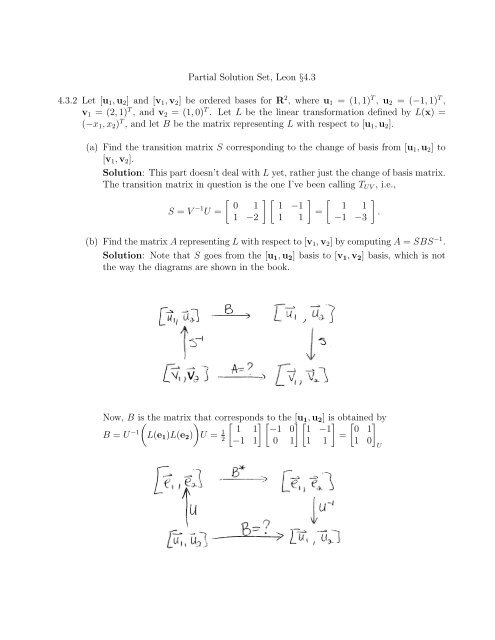
<strong>4.3.2</strong> <strong>Let</strong> [u1, u2] and [v1, v2] be ordered bases for R 2 , where u1 = (1, 1) T , u2 = (−1, 1) T ,<br />
v1 = (2, 1) T , and v2 = (1, 0) T . <strong>Let</strong> L be the linear transformation defined by L(x) =<br />
(−x1, x2) T , and let B be the matrix representing L with respect to [u1, u2].<br />
(a) Find the transition matrix S corresponding to the change of basis from [u1, u2] to<br />
[v1, v2].<br />
<strong>Solution</strong>: This part doesn’t deal with L yet, rather just the change of basis matrix.<br />
The transition matrix in question is the one I’ve been calling TUV , i.e.,<br />
S = V −1 U =<br />
� 0 1<br />
1 −2<br />
� � 1 −1<br />
1 1<br />
� �<br />
=<br />
1 1<br />
−1 −3<br />
(b) Find the matrix A representing L with respect to [v1, v2] by computing A = SBS −1 .<br />
<strong>Solution</strong>: Note that S goes from the [u1, u2] basis to [v1, v2] basis, which is not<br />
the way the diagrams are shown in the book.<br />
Now, B is the matrix that corresponds to the [u1, u2] is obtained by<br />
B = U −1<br />
� �<br />
L(e1)L(e2) U = 1<br />
� � � � � � � �<br />
1 1 −1 0 1 −1 0 1<br />
=<br />
2 −1 1 0 1 1 1 1 0<br />
�<br />
.<br />
U
Next we find S−1 = 1<br />
� �<br />
3 1<br />
. Then it is a simple matter to determine that<br />
2 −1 −1<br />
A = SBS −1 � � � � � � � �<br />
1 1 0 1 1 3 1 1 0<br />
=<br />
=<br />
.<br />
−1 −3 1 0 2 −1 −1 −4 −1<br />
V<br />
1. Verify that L(v1) = a11v1 + a21v2 and L(v2) = a12v1 + a22v2<br />
� � � � � � � �<br />
2 −2<br />
<strong>Solution</strong>: Note that L v1 = L = and on the other hand<br />
� � � �<br />
1<br />
� �<br />
1<br />
2 1 −2<br />
a11v1 + a21v2 = 1 · + (−4) = , so they match.<br />
1 0 1<br />
� � � � � � � �<br />
1 −1<br />
Also L v2 = L = and on the other hand<br />
�<br />
0<br />
�<br />
0<br />
� � � �<br />
2 1 −1<br />
a12v1 + a22v2 = 0 · + (−1) = , so they match.<br />
1 0 0<br />
4.3.3 <strong>Let</strong> L be the linear transformation on R 3 given by<br />
L(x) = (2x1 − x2 − x3, 2x2 − x1 − x3, 2x3 − x1 − x2) T ,<br />
and let A be the matrix representing L with respect to the standard basis for R 3 . If<br />
u1 = (1, 1, 0) T , u2 = (1, 0, 1) T , and u3 = (0, 1, 1) T , then [u1, u2, u3] is an ordered basis<br />
for R 3 .<br />
(a) Find the transition matrix U corresponding to the change of basis from [u1, u2, u3]<br />
to the standard basis.<br />
(b) Determine the matrix B representing L with respect to [u1, u2, u3].<br />
<strong>Solution</strong>:<br />
⎡<br />
(a) This is simply U = ⎣<br />
1 1 0<br />
1 0 1<br />
0 1 1<br />
⎤<br />
⎦ .<br />
2
(b) Somewhat surprisingly, B = U −1 AU = A. An interesting sidelight: this means that<br />
UA = AU, i.e., we have an instance of a commuting pair of matrices.<br />
4.3.4 <strong>Let</strong> L be the linear operator mapping R3 into R3 ⎡<br />
⎤<br />
defined by L(x) = Ax, where A =<br />
3 −1 −2<br />
⎣ 2 0 −2 ⎦ . <strong>Let</strong> v1 = (1, 1, 1)<br />
2 −1 −1<br />
T , v2 = (1, 2, 0) T , and v3 = (0, −2, 1) T . Find the<br />
transition matrix V corresponding to a change of basis from [v1, v2, v3] to the standard<br />
basis, and use it to determine the matrix B representing L with respect to [v1, v2, v3].<br />
⎡ ⎤<br />
1 1 0<br />
<strong>Solution</strong>: The transition matrix is V = ⎣ 1 2 −2 ⎦ . We want<br />
1 0 1<br />
B = V −1 ⎡<br />
−2 1<br />
⎤ ⎡<br />
2 3 −1<br />
⎤ ⎡<br />
−2 1 1<br />
⎤<br />
0<br />
⎡<br />
0 0<br />
⎤<br />
0<br />
AV = ⎣ 3 −1 −2 ⎦ ⎣ 2 0 −2 ⎦ ⎣ 1 2 −2 ⎦ = ⎣ 0 1 0 ⎦ .<br />
2 −1 −1 2 −1 −1 1 0 1 0 0 1<br />
4.3.5 <strong>Let</strong> L be the linear operator on P3 defined by<br />
L(p(x)) = xp ′ (x) + p ′′ (x).<br />
(a) Find the matrix A representing L with respect to [1, x, x 2 ].<br />
(b) Find the matrix B representing L with respect to basis B given by [1, x, 1 + x 2 ].<br />
(c) Find the matrix S such that B = S −1 AS.<br />
(d) Given p(x) = a0 + a1x + a2(1 + x 2 ), find L n (p(x)).<br />
(e) Given p(x) = a0 + a1x + a2(x 2 ), find L n (p(x)) (this is not in the book, but try it!).<br />
<strong>Solution</strong>:<br />
(a) We start by applying L to the basis vectors: L(1) = 0, L(x) = x, and L(x2 ) = 2x2 ⎡ ⎤+<br />
0 0 2<br />
2. The corresponding coordinate vectors become the columns of A = ⎣ 0 1 0 ⎦ .<br />
0 0 2<br />
(b) The coordinate vectors for 1 and x are unchanged, but the coordinate vector for<br />
2x2 + 2 is now (0, 0, 2) T ⎡ ⎤<br />
0 0 0<br />
, so B = ⎣ 0 1 0 ⎦ .<br />
0 0 2<br />
(c) The change of basis matrix has for its columns the vectors in R3 corresponding<br />
to each of the vectors in [1, x, 1 + x2 ] since we have to find the change of basis<br />
matrix from the arbitrary basis [1, x, 1 + x2 ] to the standard basis [1, x, x2 ⎡ ⎤<br />
]: S =<br />
1 0 1<br />
⎣ 0 1 0 ⎦ .<br />
0 0 1<br />
3
(d) The coordinate vector of p(x) is (a0, a1, a2) T B<br />
with respect to the basis B given by<br />
[1, x, 1 + x2 ]. The nth power of L is given by the nth power of B, which is simple<br />
to compute because of the simple diagonal structure of B; Bn ⎡<br />
0 0 0<br />
= ⎣ 0 1 0<br />
0 0 2n ⎤<br />
⎦ . It<br />
follows that the coordinate vector for L n (p(x)) is B n (a0, a1, a2) T = (0, a1, 2 n a2), so<br />
L n (p(x)) = a1x + 2 n a2(1 + x 2 ).<br />
(e) There isn’t a part (e), but I would like to emphasis how this B = S−1AS helps:<br />
The coordinate vector of p(x) is (a0, a1, a2) T with respect to standard basis. The<br />
nth power of L is given by the nth power of A, which is not so simple to computer<br />
since A is not diagonal as it was in part (d). However, from B = S−1AS we can<br />
find A = SBS −1 , so then A2 = (SBS −1 ) 2 = SBS −1SBS −1 = SB2S −1 . Similarly,<br />
A100 = SB100S−1 , or generally An = SBnS −1 , for all natural numbers n. Thus<br />
⎡<br />
A n = ⎣<br />
1 0 1<br />
0 1 0<br />
0 0 1<br />
⎤ ⎡<br />
⎦ ⎣<br />
0 0 0<br />
0 1 0<br />
0 0 2 n<br />
⎤ ⎡<br />
⎦ ⎣<br />
1 0 1<br />
0 1 0<br />
0 0 1<br />
which is easy to computer as a product of three matrices, instead of multiplying A<br />
by itself n times. It follows that the coordinate vector for L n (p(x)) is A n (a0, a1, a2) T<br />
which is<br />
4.3.8 Suppose that A = SΛS −1 , where Λ is a diagonal matrix with main diagonal λ1, λ2, . . . , λn.<br />
(a) Show that Asi = λisi for each 1 ≤ i ≤ n.<br />
n�<br />
(b) Show that if x = αisi, then Ak n�<br />
x =<br />
i=1<br />
i=1<br />
αiλ k i si.<br />
(c) Suppose that |λi| < 1 for each 1 ≤ i ≤ n. What happens to A k x as k → ∞?<br />
<strong>Solution</strong>:<br />
(a) For any choice of i, 1 ≤ i ≤ n, we have<br />
Asi = � SΛS −1� =<br />
si<br />
SΛ � S −1 �<br />
si<br />
= SΛei<br />
= S (Λei)<br />
4<br />
= Sλiei<br />
= λiSei<br />
= λisi.<br />
⎤<br />
⎦<br />
−1<br />
,
The reason that S −1 si = ei is because when you multiply S −1 S = I, and so when<br />
you multiply the ith column of S by S−1 you get the ith column of I, which is ei.<br />
(b) This is easily proven by induction: A0 n�<br />
x = x = αisi.<br />
Assume that A k x =<br />
n�<br />
i=1<br />
and the result follows by induction.<br />
i=1<br />
αiλ k i si for some k ∈ N. Then<br />
A k+1 x = AA k x<br />
= A<br />
=<br />
=<br />
=<br />
=<br />
n�<br />
i=1<br />
n�<br />
i=1<br />
n�<br />
i=1<br />
n�<br />
i=1<br />
n�<br />
i=1<br />
αiλ k i si<br />
Aαiλ k i si<br />
αiλ k i Asi<br />
αiλ k i λisi<br />
αiλ k+1<br />
i si,<br />
(c) Each term in the preceding sum vanishes, since if |λ| < 1 then lim<br />
k→∞ λ k = 0.<br />
4.3.9 Suppose that A = ST , where S is nonsingular. <strong>Let</strong> B = T S. Show that B is similar to<br />
A.<br />
Proof: Assume that A is as described, i.e., that A = ST and that S is nonsingular.<br />
Then<br />
B = T S = (S −1 S)T S = S −1 (ST )S = S −1 AS,<br />
so B is similar to A.<br />
A second way to present the proof above would be:<br />
Proof: Assume that A is as described, i.e., that A = ST and since S is nonsingular<br />
T = S −1 A. Then<br />
B = T S = (S −1 A)S = S −1 AS,<br />
so B is similar to A.<br />
What’s the point? Given any square S and T , with at least one of the two nonsingular,<br />
we know that it’s unlikely that ST = T S. But at least ST and T S are similar. And that<br />
(as we shall see) means that they have much in common (eigenvalues, for example).<br />
5
4.3.11 Show that if A and B are similar matrices, then det(A) = det(B).<br />
<strong>Solution</strong>: If A and B are similar, then B = S −1 AS for some nonsingular S. Now use<br />
the fact that the determinant of a product is the product of the determinants, along with<br />
the commutativity of real multiplication: det B = det(S −1 AS) = det S −1 det A det S =<br />
det S −1 det S det A = det(S −1 S) det A = det I det A = det A.<br />
6