Trans-ABySS v1.1.0: User Manual - Canada's Michael Smith ...
Trans-ABySS v1.1.0: User Manual - Canada's Michael Smith ...
Trans-ABySS v1.1.0: User Manual - Canada's Michael Smith ...

You also want an ePaper? Increase the reach of your titles
YUMPU automatically turns print PDFs into web optimized ePapers that Google loves.
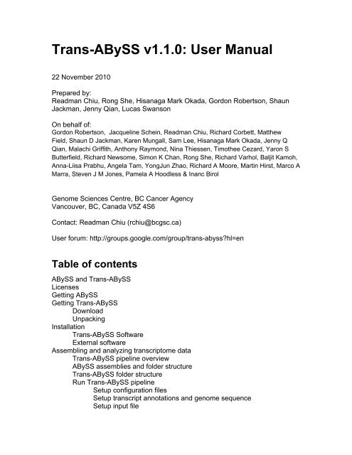
<strong>Trans</strong>-<strong>ABySS</strong> <strong>v1.1.0</strong>: <strong>User</strong> <strong>Manual</strong><br />
22 November 2010<br />
Prepared by:<br />
Readman Chiu, Rong She, Hisanaga Mark Okada, Gordon Robertson, Shaun<br />
Jackman, Jenny Qian, Lucas Swanson<br />
On behalf of:<br />
Gordon Robertson, Jacqueline Schein, Readman Chiu, Richard Corbett, Matthew<br />
Field, Shaun D Jackman, Karen Mungall, Sam Lee, Hisanaga Mark Okada, Jenny Q<br />
Qian, Malachi Griffith, Anthony Raymond, Nina Thiessen, Timothee Cezard, Yaron S<br />
Butterfield, Richard Newsome, Simon K Chan, Rong She, Richard Varhol, Baljit Kamoh,<br />
Anna-Liisa Prabhu, Angela Tam, YongJun Zhao, Richard A Moore, Martin Hirst, Marco A<br />
Marra, Steven J M Jones, Pamela A Hoodless & Inanc Birol<br />
Genome Sciences Centre, BC Cancer Agency<br />
Vancouver, BC, Canada V5Z 4S6<br />
Contact: Readman Chiu (rchiu@bcgsc.ca)<br />
<strong>User</strong> forum: http://groups.google.com/group/trans-abyss?hl=en<br />
Table of contents<br />
<strong>ABySS</strong> and <strong>Trans</strong>-<strong>ABySS</strong><br />
Licenses<br />
Getting <strong>ABySS</strong><br />
Getting <strong>Trans</strong>-<strong>ABySS</strong><br />
Download<br />
Unpacking<br />
Installation<br />
<strong>Trans</strong>-<strong>ABySS</strong> Software<br />
External software<br />
Assembling and analyzing transcriptome data<br />
<strong>Trans</strong>-<strong>ABySS</strong> pipeline overview<br />
<strong>ABySS</strong> assemblies and folder structure<br />
<strong>Trans</strong>-<strong>ABySS</strong> folder structure<br />
Run <strong>Trans</strong>-<strong>ABySS</strong> pipeline<br />
Setup configuration files<br />
Setup transcript annotations and genome sequence<br />
Setup input file
Datesets<br />
Large<br />
Small<br />
References<br />
Run trans-<strong>ABySS</strong><br />
Setting up contigs for analysis<br />
Process <strong>ABySS</strong> contigs for each k-mer assembly<br />
Create the merged assembly<br />
Using the wrapper<br />
Contig and read alignments<br />
Read alignments to contigs<br />
Contig alignments to a reference genome<br />
Aligning reads to a reference genome<br />
<strong>Trans</strong>criptome assembly analysis<br />
Identify candidate novel transcript structures<br />
Estimate gene-level expression<br />
Identify candidate gene fusion events<br />
Identify putative chimeric transcripts<br />
Additional <strong>Trans</strong>-<strong>ABySS</strong> functions<br />
Identify candidate SNVs and INDELs<br />
Identify candidate polyadenylation sites<br />
Insr_UTR<br />
Polyadenylation site analysis<br />
<strong>ABySS</strong> and <strong>Trans</strong>-<strong>ABySS</strong><br />
<strong>ABySS</strong> is a de Bruijn graph-based short-read assembler that can process<br />
genome or transcriptome sequence data (Simpson et al. 2009, Birol et al. 2009).<br />
<strong>Trans</strong>-<strong>ABySS</strong> is an analysis pipeline for post-processing <strong>ABySS</strong> assemblies of<br />
transcriptome sequencing data. It addresses varying transcript expression levels<br />
by processing multiple assemblies across a range of k values (Robertson et al.<br />
2010).<br />
The current pipeline can map assembled contigs to annotated transcripts (e.g.<br />
RefSeq, Ensembl,...), and can identify candidate novel splicing events such<br />
as exon-skipping, novel exons, retained introns, novel introns, and alternative<br />
splicing. It can also extract candidate SNVs, INDELs, and gene fusion events<br />
from contig alignment data. It also finds putative chimeric transcript events and<br />
candidate polyA sites.<br />
The <strong>Trans</strong>-<strong>ABySS</strong> pipeline consists of a) Perl wrapper scripts; b) Python, Perl<br />
and bash scripts; and c) command line applications. The pipeline can be run on<br />
any POSIX-compliant platform. Processing large datasets will require a computer
cluster.<br />
Licenses<br />
<strong>ABySS</strong> and <strong>Trans</strong>-<strong>ABySS</strong> are released under the terms of the BC Cancer<br />
Agency software license agreement. http://www.bcgsc.ca/platform/bioinfo/<br />
license/bcca_2010<br />
Getting <strong>ABySS</strong><br />
The <strong>Trans</strong>-<strong>ABySS</strong> pipeline will process outputs from <strong>ABySS</strong> v1.1.2+. <strong>ABySS</strong><br />
v1.1.1 was used for the Nature Methods publication. Source code for v1.1.1 and<br />
for the most current release of <strong>ABySS</strong> is available at:<br />
www.bcgsc.ca/platform/bioinfo/software/abyss<br />
The <strong>ABySS</strong>-users discussion group is available at:<br />
http://groups.google.com/group/abyss-users<br />
<strong>ABySS</strong> can be compiled to run on any POSIX-compliant system. Use the<br />
following commands to read <strong>ABySS</strong> man pages:<br />
man doc/abyss-pe.1<br />
man doc/ABYSS.1<br />
Getting <strong>Trans</strong>-<strong>ABySS</strong><br />
1. Download<br />
The pipeline software can be downloaded from:<br />
http://www.bcgsc.ca/platform/bioinfo/software/trans-abyss<br />
2. Unpacking<br />
After unpacking, files will be automatically organized into five folders:<br />
analysis Contains Python modules and Perl scripts that are used for<br />
analyzing <strong>ABySS</strong>-assembled transcriptome assemblies.
annotations Contains transcript and repeat annotation files used in analysis.<br />
It is organized by reference genome assembly (e.g. hg18,<br />
mm9, etc).<br />
configs Contains configuration files (.cfg) that are used for running the<br />
trans-<strong>ABySS</strong> pipeline.<br />
utilities Contains Python modules (.py) and <strong>ABySS</strong>-related binaries that<br />
support the analysis modules.<br />
wrappers Contains Perl scripts (.pl) that are wrappers for running the<br />
<strong>Trans</strong>-<strong>ABySS</strong> pipeline.<br />
sample_data Contains a small sample dataset that can be used for testing<br />
Installation<br />
1. <strong>Trans</strong>-<strong>ABySS</strong> Software<br />
Most of the software is written in Python. Because <strong>Trans</strong>-<strong>ABySS</strong> uses Pysam<br />
(http://code.google.com/p/pysam/) to parse .sam files, Python 2.6 or later is<br />
required.<br />
The wrapper scripts for running the pipeline are written in Perl. All Perl5 versions<br />
should work. To use the wrappers, you must add to the Perl path a simple<br />
custom configuration module for parsing config files. This module is supplied in<br />
the “wrappers” folder.<br />
By setting the following environmental variables you should be ready to run the<br />
<strong>Trans</strong>-<strong>ABySS</strong> software:<br />
export TRANSABYSS_PATH=/home/user/trans-<strong>ABySS</strong><br />
export PYTHONPATH=.:$PYTHONPATH:$TRANSABYSS_PATH<br />
export PERL5LIB=.:$PERL5LIB:$TRANSABYSS_PATH/wrappers<br />
For convenience, a “setup” file is included in the trans-<strong>ABySS</strong> root<br />
folder, which includes the setup of the environmental variables.<br />
Change “TRANSABYSS_PATH” to your own trans-<strong>ABySS</strong> directory. Then<br />
type “source setup” at the command line.<br />
In addition, the reference genomes and their annotations that are used in<br />
analysis should be present in the "annotations" folder. For each reference<br />
genome, there should be a "genome.fa" file in its corresponding folder. To run<br />
chimeric transcript event finder code, a “2bit” format genome file is used. Please<br />
refer to Section 4.2 for details of required annotation files. The current trans-<br />
<strong>ABySS</strong> package provides annotation files for two reference genomes: “hg18”
and “mm9”, which can be downloaded separately from the software download<br />
page. For analysis on other genomes, please set up their annotation folders in<br />
the same fashion.<br />
For convenience, the trans-<strong>ABySS</strong> software package provides two scripts<br />
in the root directory: “setup_hg18” and “setup_mm9”, to allow automatic<br />
download and setup of the “hg18” and “mm9” annotation folders. Simply<br />
type “source setup_hg18” and/or “source setup_mm9” to download and set<br />
up annotations for hg18 and mm9.<br />
The ‘External software’ section (below) lists other required software.<br />
2. External Software<br />
In addition to Python and Perl, <strong>Trans</strong>-<strong>ABySS</strong> requires the following:<br />
1. Blat (http://users.soe.ucsc.edu/~kent/src/)<br />
Blat is used for:<br />
1. Merging: pairwise alignment of contigs to remove redundant contigs.<br />
2. Aligning contigs to a reference genome.<br />
2. Pysam (http://code.google.com/p/pysam/)<br />
Pysam is used for parsing .bam files for parsing read-to-contig alignments.<br />
3. BioPython (http://www.biopython.org/wiki/Download)<br />
Biopython is used in two parts of <strong>Trans</strong>-<strong>ABySS</strong> analysis:<br />
1. <strong>Trans</strong>lating DNA sequence into peptide sequence for identifying<br />
potential open reading frames.<br />
2. The “NCBIStandalone.py" module is used for parsing Blast-format<br />
output from Blat to extract candidate single nucleotide variants (SNVs)<br />
and insertion-deletions (INDELs). After downloading the module, edit the<br />
following line in so that HSPs of all scores will be parsed:<br />
r"Score =\s*([0-9.e+]+) bits \(([0-9]+)\)", line,<br />
should be changed to:<br />
r"Score =\s*([0-9.e+-]+) bits \(([0-9-]+)\)", line,<br />
4. Samtools (http://samtools.sourceforge.net/)<br />
Samtools is used for merging and indexing read alignment files.
5. Bowtie (http://bowtie-bio.sourceforge.net/index.shtml)<br />
Bowtie is used in single-end alignment for aligning reads to contigs.<br />
6. The CPAN Perl module Config::General, IO::Compress, Set::IntSpan<br />
http://search.cpan.org/~tlinden/Config-General-2.49/General.pm<br />
http://search.cpan.org/~pmqs/IO-Compress-2.030/lib/IO/Uncompress/<br />
Gunzip.pm<br />
http://search.cpan.org/dist/Set-IntSpan/<br />
IO::Compress is only required if the input reads are gzipped or bzipped.<br />
The Config::General and IO::Compress modules are used by the<br />
polyadenylation site scripts. The Config::General and Set::IntSpan module is<br />
used by the chimeric transcript event finder scripts.<br />
7. BWA (http://bio-bwa.sourceforge.net/bwa.shtml)<br />
BWA is used to align PAM and EJ reads to known transcript sequences in<br />
the polyadenylation site analysis.<br />
Assembling and analyzing transcriptome data<br />
1. <strong>Trans</strong>-<strong>ABySS</strong> Pipeline Overview<br />
Because transcriptome samples typically contain transcripts with a wide range of<br />
expression levels, and assemblies generated with different k-mer lengths perform<br />
differently in capturing transcripts expressed at different levels, we recommend<br />
using a wide range of k-mer values to assemble read data from an RNA-seq<br />
library (Robertson et al. 2010). Currently, for a read length L, we typically use a<br />
range from L/2 to L-1 for libraries with L 50 bp.<br />
<strong>Trans</strong>-<strong>ABySS</strong> starts with a set of <strong>ABySS</strong> assemblies for a range of k values.<br />
It processes them into a merged assembly, which is then used to generate<br />
alignments, identify novel events and perform other analyses. Figure 1 shows an<br />
overview of the pipeline.
Figure 1. <strong>Trans</strong>-<strong>ABySS</strong> pipeline overview.
2. <strong>ABySS</strong> assemblies and folder structure<br />
<strong>Trans</strong>-<strong>ABySS</strong> expects the output from <strong>ABySS</strong> multi-k assemblies for each library<br />
to be organized as follows: a single parent folder is used to hold all k-assemblies,<br />
where each subfolder is named “kn” (n is the value of k, e.g. k35) and stores<br />
the <strong>ABySS</strong> assembly output files for that particular k value (Fig. 2). In addition,<br />
a simple text file named “in” should be present in the <strong>ABySS</strong> assembly folder,<br />
which lists all the paths of all input read files.<br />
LIB0001/<br />
k1/<br />
k2/<br />
…<br />
in<br />
LIB-contigs.fa<br />
LIB-1.adj<br />
LIB-1.fa<br />
LIB-4.adj<br />
[other <strong>ABySS</strong> output files]<br />
LIB-contigs.fa<br />
LIB-1.adj<br />
LIB-1.fa<br />
LIB-4.adj<br />
[other <strong>ABySS</strong> output files]<br />
Figure 2. The <strong>ABySS</strong> assembly folder structure that <strong>Trans</strong>-<strong>ABySS</strong> expects.<br />
Each ‘k’ folder holds the output of an <strong>ABySS</strong> assembly that was generated using<br />
that k value. Here, schematic folder ‘k’ names are shown; typical names might<br />
be: k26, k27, ....<br />
The read files specified by the “in” file can be in any of the following formats:<br />
bam, qseq, export, or fastq. They can be compressed using gzip or bzip2<br />
(with “.gz” or “.bz2” extensions). Fig. 3 shows an example “in” file.<br />
/archive/solexa1_4/analysis2/HS1136/3153YAAXX_2/<br />
3153YAAXX_2_1_export.txt.gz<br />
/archive/solexa1_4/analysis2/HS1136/3153YAAXX_2/<br />
3153YAAXX_2_2_export.txt.gz<br />
/archive/solexa1_4/analysis3/HS1136/42HVVAAXX_1/<br />
42HVVAAXX_1_1_export.txt.gz<br />
/archive/solexa1_4/analysis3/HS1136/42HVVAAXX_1/<br />
42HVVAAXX_1_2_export.txt.gz<br />
/archive/solexa1_4/analysis3/HS1136/42HVVAAXX_2/<br />
42HVVAAXX_2_1_export.txt.gz<br />
/archive/solexa1_4/analysis3/HS1136/42HVVAAXX_2/<br />
42HVVAAXX_2_2_export.txt.gz
Figure 3. An example “in” file that specifies paths to all input read files.<br />
Once the “in” file is created, <strong>ABySS</strong> can be run with multiple k values on the<br />
same set of read files. For convenience, an example shell script “run-abyss”<br />
is included in <strong>Trans</strong>-<strong>ABySS</strong> “utilities” folder, which demonstrates how to<br />
generate <strong>ABySS</strong> multi-k assemblies in the required folder structure:<br />
for k in {26..49}; do mkdir k$k; cd k$k; abyss-pe<br />
in=`paste -sd' ' in` OVERLAP_OPTIONS=--no-scaffold<br />
SIMPLEGRAPH_OPTIONS=--no-scaffold E=0 n=10 v=-v; cd ..;<br />
done<br />
The following are example scripts to run <strong>ABySS</strong> on a computer cluster and<br />
generate multi-k assemblies in the required folder structures using qsub:<br />
Script: utilities/qsub-l50-64<br />
#!/bin/sh<br />
set -eu<br />
qsub -N `basename $PWD` -t 33-49 ../qsub-l50-k64<br />
Script: utilities/qsub-l50-k64<br />
#!/bin/env qsub<br />
#$ -q mpi.q<br />
#$ -pe openmpi-1.3.1 16<br />
#$ -l hostname=qn*<br />
##$ -l mem_used=300M<br />
setenv PATH [PATH-TO-ABYSS-BINARIES]:$PATH<br />
setenv in `paste -sd' ' in`<br />
mkdir k$SGE_TASK_ID && cd k$SGE_TASK_ID && \<br />
abyss-pe OVERLAP_OPTIONS=--no-scaffold<br />
SIMPLEGRAPH_OPTIONS=--no-scaffold E=0 n=10 v=-v<br />
Note that <strong>ABySS</strong> scaffold option produces sequences with Ns and ambiguity<br />
codes, which may cause difficulty in some process of the current trans-<strong>ABySS</strong><br />
pipeline. Thus we recommend either running <strong>ABySS</strong> with scaffold option off<br />
or breaking scaffolds after <strong>ABySS</strong> assembly is done. For more help on how to<br />
generate <strong>ABySS</strong> multi-k assemblies or other <strong>ABySS</strong>-related problems, please<br />
refer to the <strong>ABySS</strong> help group at http://groups.google.com/group/abyss-users.<br />
3. <strong>Trans</strong>-<strong>ABySS</strong> folder structure<br />
<strong>Trans</strong>-<strong>ABySS</strong> and <strong>ABySS</strong> have similar working directory structures (Fig.
4). The <strong>Trans</strong>-<strong>ABySS</strong> folder structure can be set up by running “transabyss”<br />
or “setup.pl”, both of which are in the “wrappers” folder (see<br />
Section 3.3 below). Each k-mer sub-folder should initially be empty, and will be<br />
populated by the “setup.pl” script to hold the processed assembly file from<br />
the corresponding <strong>ABySS</strong> k-mer assembly. The other directories are used to<br />
hold various <strong>Trans</strong>-<strong>ABySS</strong> output files, which will be discussed in detail in the<br />
following sections.<br />
Project/<br />
Library/<br />
Reads_to_genome/<br />
Reads_to_genome.bam<br />
Assembly/<br />
Abyss-1.2.1/<br />
source -> <strong>ABySS</strong> assembly path<br />
k1/<br />
Library-contigs.fa<br />
k2/<br />
Library-contigs.fa<br />
…<br />
merge/<br />
Library-contigs.fa<br />
reads_to_contigs/<br />
tracks/<br />
novelty/<br />
fusions/<br />
anomalous_contigs/<br />
Figure 4. A typical <strong>Trans</strong>-<strong>ABySS</strong> working folder.<br />
4. Running the <strong>Trans</strong>-<strong>ABySS</strong> Pipeline<br />
4.1 Set up configuration files<br />
<strong>Trans</strong>-<strong>ABySS</strong> analyses are performed on individual libraries, i.e. short-read<br />
sequencing datasets. However, to support work on a project that involves<br />
multiple related libraries (e.g. tens of patients for a disease), sets of libraries can<br />
be organized under a common project directory, and can share common run<br />
configuration settings. Settings are specified in configuration files, as follows.<br />
The wrapper scripts use the following configuration files (in “configs” folder) to<br />
run the pipeline:<br />
● projects.cfg
For each project, the user specifies the reference genome and the<br />
top-level ‘project’ directory (Fig. 5). A ‘project’ directory will contain<br />
a subdirectory for each of its libraries. In “projects.cfg”, default<br />
parameters for each script are specified in the “default” section. Defaults<br />
can be overridden by values set with each project. Uppercase words<br />
(e.g. MERGINGDIR) are used by calling scripts as templates that will be<br />
automatically replaced with appropriate values during a pipeline run.<br />
[default]<br />
merge.pl: VERDIR LIB contigs MERGINGDIR<br />
align_parser.py: BLAT_DIR blat -n 1 -u -m 90 -d -k<br />
TRACK_NAME -o PSL -f CONTIGS<br />
...<br />
[projectA]<br />
topdir: /projects/projectA<br />
reference: hg18<br />
[projectB]<br />
...<br />
Figure 5. Example organization of “projects.cfg”<br />
● binaries.cfg<br />
Paths to external software are specified in “software: path” format, with<br />
one line for each executable (Fig. 6). An example file is provided in<br />
the distribution. Note in the example file, two versions of “python” are<br />
specified: “python” points to the executable of the correct version of<br />
python that runs on GSC’s cluster, and “python_xhost” points to the<br />
executable of the version of python that runs locally. Please replace all<br />
paths to point to proper binaries in your own computing environment. Do<br />
not change the name of software (the part before “:”).<br />
[binaries]<br />
python: /gsc/software/linux-x86_64/python-builder-2.6.4/bin/<br />
python<br />
python_xhost: /home/rshe/bin/bin/python<br />
perl: /usr/local/bin/perl5.8.3<br />
blat: /home/pubseq/BioSw/blat/blat34/blat<br />
exonerate: /home/pubseq/BioSw/exonerate/exonerate-2.2.0-x86_64/<br />
bin/exonerate<br />
bwa: /home/pubseq/BioSw/bwa/bwa-0.5.6/bwa<br />
bowtie: /home/rchiu/bin/bowtie-0.12.5/bowtie<br />
bowtie_build: /home/rchiu/bin/bowtie-0.12.5/bowtie-build<br />
samtools: /home/pubseq/BioSw/samtools/0.1.6/samtools<br />
export2fq: /home/pubseq/BioSw/Maq/maq-0.7.1_x86_64-linux/<br />
scripts/fq_all2std.pl export2std<br />
biopython: /home/rchiu/python/biopython-1.52
mqsub: /opt/mqtools/bin/mqsub<br />
Figure 6. Example of “binaries.cfg”<br />
● cluster.cfg<br />
Specify cluster job settings including the memory requirement for running<br />
different scripts on cluster, and the file used for each reference genome<br />
(FIg. 7). This file is required when running jobs on a cluster.<br />
[memory]<br />
merge.pl: 1G<br />
fusion.py: 1G<br />
model_matcher.py: 10G<br />
reads_to_contigs.py: 1G<br />
align_parser.py: 1G<br />
cluster_align.py: 5G<br />
gene_coverage.py: 1G<br />
[genomes]<br />
hg18: /var/tmp/genome/lymphoma/ucsc-hg18.fa<br />
mm9: /var/tmp/genome/mouse/mm9_build37_mouse.fasta<br />
Figure 7. Example of “cluster.cfg”<br />
● align.cfg<br />
Specify parameters used by each aligner when contigs are aligned to the<br />
reference genome.<br />
● model_matcher.cfg<br />
Specify settings of annotations for “model_matcher.py”, for finding<br />
novel transcripts and transcript events, relative to reference transcript<br />
annotations (Fig. 8). Each section specifies the annotation files and their<br />
order for a reference genome. See section 4.4.3A for more details.<br />
[hg18]<br />
k: knownGene_ref.txt<br />
e: ensGene_ref.txt<br />
r: refGene.txt<br />
a: acembly_ref.txt<br />
x: ensg.txt<br />
order: k,e,r,a<br />
[mm9]<br />
k: knownGene_ref.txt<br />
e: ensGene_ref.txt<br />
r: refGene.txt<br />
a: acembly_ref.txt<br />
order: k,e,r,a
Figure 8. Example of “model_matcher.cfg”<br />
● submitjobs.sh<br />
The “submitjobs.sh” script in the “utilities” folder is used to run<br />
jobs on a computer cluster. The GSC cluster is currently a ~2000+ core<br />
(CPUs) Beowulf-style cluster running Red Hat Enterprise Linux 4. The<br />
infrastructure consists of a headnode to which users submit jobs, and<br />
the rest of the cluster consists of compute nodes that are involved only in<br />
computation. The headnode, called “apollo”, runs OSCAR 5.0pre with Sun<br />
Grid Engine 6.1u3. We submit jobs to apollo with this command:<br />
submitjobs.sh apollo /opt/mqtools/bin/mqsub <br />
<br />
Please adjust “submitjobs.sh” to be appropriate to your cluster.<br />
4.2 Set up transcript annotations and genome sequence<br />
<strong>Trans</strong>-<strong>ABySS</strong> compares genome alignments of assembled contigs to known<br />
annotations to discover transcript variants that are novel relative to reference<br />
transcript annotations.<br />
<strong>Trans</strong>cript annotation files are downloaded from the UCSC genome browser.<br />
Annotation files are organized by reference genome (Fig. 9). Currently trans-<br />
<strong>ABySS</strong> comes with “hg18” and “mm9” annotations (under “annotations”<br />
folder) that include Ensembl, UCSC, Aceview and Refseq transcripts.<br />
annotations/<br />
hg18/<br />
genome.fa -> ucsc-hg18.fa<br />
knownGene.txt<br />
knownGene_ref.txt<br />
knownGene_ref.idx<br />
knownGene_exons.txt<br />
hg18.2bit<br />
hg18_all_rmsk.coord<br />
RNA.repeat.txt<br />
splice_motives.txt<br />
…<br />
mm9/<br />
…<br />
shared/<br />
splice_motives.txt<br />
README<br />
Figure 9. Organization of the “annotations” folder.
4.2.1 Reference Genome<br />
The reference genome fasta file is expected to be either copied or linked to<br />
genome folder as “genome.fa”. In addition, a “.2bit” genome<br />
file is needed when running scripts that find chimeric transcript events (transabyss<br />
stage 8 and 9), where is the reference name such as “hg18”<br />
or “mm9”.<br />
4.2.2 <strong>Trans</strong>cript Annotations<br />
<strong>Trans</strong>cript annotation files<br />
(“knownGene.txt”, “ensGene.txt”, “acembly.txt”) (downloaded<br />
from UCSC) need to be modified slightly to include the common<br />
gene names at the end of each record<br />
(“knownGene_ref.txt”, “ensGene_ref.txt”, “acebmly_ref.txt”).<br />
The “refGene.txt” file (also downloaded from UCSC) does not require such<br />
processing. The “README” file in the “annotations” folder describes how to do<br />
this.<br />
4.2.3 Indexes (“.idx” files)<br />
The transcript annotation files are indexed by genomic locations to expedite the<br />
searching and matching of contigs. Indexing is achieved by running the scripts<br />
in the “analysis/annotations” folder, one for each transcript model. For<br />
example, to index Ensembl transcripts, run the following command:<br />
python ~mapper/trans-<strong>ABySS</strong>/analysis/annotations/<br />
ensembl.py ~mapper/trans-<strong>ABySS</strong>/annotations/hg18/<br />
ensGene.txt -i ~mapper/trans-<strong>ABySS</strong>/annotations/hg18/<br />
ensGene.idx<br />
Currently, the following four scripts are supplied: ensembl.py, knownGene.py<br />
(for ucsc known genes), aceview.py (aceview genes), refGene.py (for refseq<br />
genes).<br />
<strong>Trans</strong>cript model files with other formats can be used if you create a custom<br />
parser. This can be easily done by modifying any of the existing parsers in<br />
the “analysis/annotations/” folder.<br />
4.2.4 Exon coordinates<br />
To find chimeric transcript events (trans-abyss stage 8 and 9, see Section 4.4),<br />
each genome should have the exon coordinate annotation file (*-exons.txt).<br />
There can be multiple exon coordinate files, with one file being used as the<br />
primary annotation (required) and multiple other files can be used as secondary
annotations (optional) that provide support for putative events that are detected<br />
based on the primary annotation.<br />
These files are generated based on transcript annoation files downloaded<br />
from UCSC. The “README” file in the “annotations” folder describes how to<br />
generate them from UCSC files.<br />
4.2.5 Repeat annotations<br />
The chimeric transcript finder script (trans-abyss stage 8 and 9) is also<br />
able to take into consideration of repeats in annotation. To enable this,<br />
each genome should have a coordinate file that contains coordinates of all<br />
repeats (_all_rmsk.coord) and/or coordinate file for RNA repeats<br />
(RNA.repeat.txt).<br />
These files are generated using repeatmasker files downloaded from UCSC.<br />
The “README” file in the “annotations” folder also contains description on how<br />
to generate them.<br />
An example config file can be seen at “sample_data/Insr_UTR/Insr_UTR/<br />
Assembly/current/anomalous_contigs/ver_15.5.0/config”, which lists the<br />
annotation files that are used by the chimeric transcript event finder script.<br />
4.2.6 Splice motifs<br />
The “splice_motives.txt” file specifies motives of known splice sites for<br />
each genome. It is used by “align_parser.py” and “model_matcher.py”<br />
(see Section 4.4.3A) for determining whether a splice site is novel or known.<br />
There is also a shared “splice_motives.txt” file (under “shared” folder) that<br />
can be used as common splice motifs, and the “splice_motifs.txt” file in<br />
each reference genome can be a symbolic link to this file.<br />
4.3 Set up the input file<br />
The wrapper scripts take an input file as the argument (Fig. 10). The input file<br />
specifies the libraries that need to be processed. Each library is specified by 5<br />
fields in one line:<br />
<br />
The fields are separated by spaces. The is the<br />
name of the parent folder that holds all <strong>ABySS</strong> k-assemblies for that library,<br />
where each k-assembly is in a subfolder kn (see Fig. 2). is<br />
the smallest read length in the library (note that it is possible to have different-
length reads in one library). If is not specified, it is defaulted<br />
to 50.<br />
LIB0001 1.2.1 /projects/<strong>ABySS</strong>/assemblies/LIB0001 projectA 50<br />
LIB0002 1.2.1 /projects/<strong>ABySS</strong>/assemblies/LIB0002 projectA 50<br />
LIB0003 1.2.1 /projects/<strong>ABySS</strong>/assemblies/LIB0003 projectA 75<br />
Figure 10. Example input file.<br />
Note that library names should be unique in the same input file. To process a<br />
library with different parameters (e.g. with different <strong>ABySS</strong>-versions), each run<br />
should be put in a different input file.<br />
4.4 Running trans-<strong>ABySS</strong><br />
The current pipeline can be run with a wrapper script: “trans-abyss” (in<br />
the “wrappers” folder). It carries out analysis work in 9 stages:<br />
1. generate the transcriptome assembly<br />
1.1 set up the <strong>Trans</strong>-<strong>ABySS</strong> folder structure (as in Section 3 above);<br />
1.2 process each <strong>ABySS</strong> k-mer assembly (see Section 4.4.1A below);<br />
1.3 merge all k-mer assemblies into one assembly (see Section 4.4.1B<br />
below);<br />
2. align reads to contigs (see Section 4.4.2A below);<br />
3. align contigs to the genome (see Section 4.4.2B below);<br />
4. filter contigs-to-genome alignments and generate a track file that can be<br />
loaded to UCSC browser as a custom track (see Section 4.4.3A below);<br />
5. find candidate novel transcript events (see Section 4.4.3A below);<br />
6. report gene expression levels (see Section 4.4.3B below).<br />
7. find candidate fusion genes (see Section 4.4.3C below).<br />
8. find putative chimeric transcript events (see Section 4.4.3D below).<br />
9. group and filter putative chimeric transcript events (see Section 4.4.3D).<br />
Each stage depends on the completion of previous stages. Please refer to the<br />
pipeline overview for the workflow (Fig. 1).<br />
To run “trans-abyss”, use the following command:<br />
trans-abyss [options] <br />
where “input-file” is the input file described in Section 4.3 above. Specify the<br />
stage number to run trans-<strong>ABySS</strong> in corresponding stage: “-1”, “-2”, “-3”, “-4”, “-<br />
5”, “-6”, “-7”, “-8” or “-9”.
The options are as follows:<br />
-c <br />
name of the cluster head node to submit jobs (if applicable). For<br />
large datasets, it is necessary to run the jobs on a cluster.<br />
-s <br />
“start library”, i.e. the name of the first library to be processed<br />
in the list of libraries in the input file; can be used in combination<br />
with “-num” option (see below)<br />
-n <br />
number of libraries to process starting from "start library". Use<br />
this option in combination with “-start” option to specify the<br />
libraries that need to be processed.<br />
For example, given an input file as shown in [Figure 10], use “start<br />
LIB0002 -num 2” to start from library “LIB0002” and<br />
process 2 libraries, i.e. LIB0002 and LIB0003.<br />
If only “-start” option is specified, and “-num” is not specified,<br />
then all libraries from the start library onwards will be processed.<br />
-l <br />
library that needs to be processed (for processing single library).<br />
If only a single library needs to be processed, use this option<br />
instead of “-start” and “-num” combination.<br />
Running “trans-abyss” without “-start”, “-num”, or “-lib” options<br />
will process all libraries in the input file.<br />
-h | --help<br />
Print help message.<br />
--version<br />
Print version message.<br />
Note that most scripts in trans-<strong>ABySS</strong> package can be run with “-h”, “--help” or “-man”<br />
option to get help on the description and usage of the script.<br />
4.4.1 Setting up contigs for analysis<br />
A. Processing <strong>ABySS</strong> contigs for each k-mer assembly<br />
For each assembly, a working set of contigs will comprise the following:<br />
- all paired-end contigs; “Paired-end contigs” are contigs that were assembled<br />
during the pair-end stage of <strong>ABySS</strong> (Simpson et al. 2009).<br />
- all junction contigs; “Junction contigs” are single-end contigs that have one<br />
and only one neighbour on either side in the <strong>ABySS</strong> assembly graph and should<br />
represent the lesser-expressed branch of a heterozygous allele (indels, splice<br />
variants, etc) in the transcriptome. Junction contigs are fully extended on either<br />
side and the extended contigs that are bigger than the read length of the library<br />
(or the minimum if multiple read lengths exist) are kept .
- single-end contigs of length greater than 150bp;<br />
- single-end contigs that are not “islands” and are between (2k-1)bp and 150bp in<br />
length. “Islands” are contigs that have no neighbours in the <strong>ABySS</strong> graph.<br />
The contig set can be generated by running “assembly.py” in the “utilities”<br />
folder:<br />
assembly.py –d /k50 –o<br />
/k50/library-contigs.fa –k<br />
50 -j <br />
Running this command for each <strong>ABySS</strong> k-mer assembly will generate a single<br />
FASTA file (named “LIBRARY-contigs.fa”) in the corresponding trans-<strong>ABySS</strong> kmer<br />
directory. This filtered contig set will be used for all downstream analysis.<br />
“assembly.py” makes use of two <strong>ABySS</strong>-related programs “MergeContigs”<br />
and “SimpleGraph” which are included in trans-<strong>ABySS</strong> “utilities” folder.<br />
The “MergeContigs” program is the same program as in the <strong>ABySS</strong> package<br />
and can also be downloaded from <strong>ABySS</strong> download page. The “SimpleGraph”<br />
program is different from the version that is included in the <strong>ABySS</strong> package, thus<br />
the source file “SimpleGraph.cpp” is also included in the “utilities” folder if there is<br />
need to re-compile it.<br />
Note: “assembly.py” reads from several <strong>ABySS</strong> files in addition to the final<br />
<strong>ABySS</strong> fasta file, including “library-4.fa”, and “library-4.adj”. To process singleend<br />
<strong>ABySS</strong> assemblies that do not have “library-4.adj”, please create a symbolic<br />
link “library-4.adj” in the <strong>ABySS</strong> assembly folder that points to “library-3.adj”.<br />
B. Creating the merged assembly<br />
After each assembly has been processed, sets of contigs for assemblies across<br />
a range of k values are then merged to create a smaller, non-redundant contig<br />
set. The merging algorithm (“merge.pl”), which is described in the manuscript<br />
(Robertson et al. 2010), uses Blat to perform iterative pairwise alignments<br />
between assemblies:<br />
merge.pl contigs<br />
/merge/merging<br />
The final result is another FASTA file (also named “LIBRARY-contigs.fa”, but<br />
under the “merge” sub-folder) that consists of the non-redundant contig set from<br />
all k-mer assemblies.<br />
C. Using the wrapper<br />
For convenience, the wrapper script “trans-abyss” is set up to<br />
call “assembly.py” and “merge.pl” automatically in its stage “-1” as follows:
trans-abyss [options] -1<br />
The options are specified in Section 4.4 above. This command will run through all<br />
k-mer assemblies and merge the results into the final FASTA file.<br />
4.4.2 Contig and read alignments<br />
A. Read alignments to contigs<br />
Read alignments to contigs are required for providing evidence ‘support’ for<br />
novel transcript events, and for estimating gene-level expression. <strong>Trans</strong>-<strong>ABySS</strong><br />
currently uses Bowtie in single-end mode to perform read-contig alignments.<br />
Because contigs can overlap, we allow multi-mapping, but require exact match<br />
alignments.<br />
The wrapper script “trans-abyss” can be used to perform reads-to-contigs<br />
alignments as follows:<br />
trans-abyss [options] -2<br />
B. Contig alignments to a reference genome<br />
All the analyses described below (except for polyadenylation sites) require that<br />
assembled contigs be aligned to the reference genome. <strong>Trans</strong>-<strong>ABySS</strong> currently<br />
supports Blat and exonerate aligners. However, outputs from other aligners<br />
that can generate .psl outputs (e.g. GMAP) can be treated as Blat outputs (by<br />
specifying the aligner as “blat” when required) and so can be processed by trans-<br />
<strong>ABySS</strong>.<br />
As noted in the manuscript (Robertson et al. 2010), to minimize the time required<br />
to review candidate novel transcript events, it is important that a contig aligner<br />
have a low error rate, and that its error rate be addressed.<br />
Because even after merging there will typically be a large number of<br />
contigs, contig alignments are usually performed in parallel on a computer<br />
cluster. Computing systems at different laboratories will differ, and<br />
the “submitjobs.sh” script in “utilities” should be tailored by users to suit<br />
their cluster configuration.<br />
To run BLAT alignments on a cluster, we split the merged assembly file into<br />
many smaller files, and run each job independently. The current default is<br />
to separate the assembly into 1,000 contigs per file. These files and their<br />
corresponding cluster job scripts and output can be found in the “merge/<br />
cluster/” subdirectory in the trans-<strong>ABySS</strong> working directory (Fig.
4):<br />
merge/cluster//input<br />
merge/cluster//jobs<br />
merge/cluster//output<br />
The “trans-abyss” wrapper script can be used to perform contig-to-genome<br />
alignments as follows:<br />
trans-abyss [options] -3<br />
Some alignment jobs may not finish successfully on the cluster. To check<br />
whether all BLAT alignment jobs for a certain library are finished completely, use<br />
the tool “check_complete_blat.pl” (supplied in the “utilities” folder) as<br />
follows:<br />
check_complete_blat.pl <br />
is the name of the directory that holds the inputs, job scripts, and<br />
outputs of the blat jobs.<br />
C. Aligning reads to a reference genome<br />
Mate-pair read alignments to a reference genome are directly used as supporting<br />
evidence to rank fusion gene candidates. A fusion candidate that is well<br />
supported by mate-pairs will be prioritized for manual review.<br />
The current pipeline does not include code for handling exon-exon junctions<br />
for such read alignments. For the results in the publication, we make a BWAaligned<br />
.bam format file, and a .bigWig file derived from it, available for download<br />
from the <strong>Trans</strong>-<strong>ABySS</strong> software v1.0 download page. These were generated with<br />
an internal GSC pipeline (unpublished).<br />
4.4.3 <strong>Trans</strong>criptome assembly analysis<br />
<strong>Trans</strong>-<strong>ABySS</strong> currently offers the following functionality.<br />
A. Identify candidate transcript structures that are novel relative to one or<br />
more sets of annotated transcript models (e.g. RefSeq, Ensembl, …).<br />
We recommend filtering contig alignments to retain only the best alignment that<br />
is unique (i.e. a contig cannot align to multiple genomic locations with the same
score) and covers the majority of the length of the contig (e.g. 90%):<br />
python align_parser.py blat_output_dir/blat_output_file<br />
blat -n 1 -u m90 -d -k “track name” -o filtered.psl -f<br />
merged_contigs.fa<br />
The wrapper script “trans-abyss” can be used to run this job:<br />
trans-abyss [options] -4<br />
After filtering, the resulting PSL-format file can be loaded into the UCSC genome<br />
browser for review, and can also be compared to reference transcript model files<br />
(e.g. in UCSC gene table format) by the “model_matcher.py” script in order to<br />
find novel transcripts and transcript events in the contig alignments:<br />
model_matcher.py filtered_track.psl genome -l -d -o<br />
output_dir -f merged_contigs.fa -r<br />
The wrapper script “trans-abyss” can be used to do this job by specifying<br />
stage “-5”:<br />
trans-abyss [options] -5<br />
The output directory will contain:<br />
1. “mapping.txt” – details the mappings of contigs to known transcripts<br />
2. “events.txt” – reports novel transcript variants relative to all transcript models<br />
(e.g. skipped exons, novel exons, …)<br />
3. “events.bed” – novel transcript variants in bed format<br />
4. “coverage.txt” – transcript coverage statistics<br />
The “mapping.txt” file is a text file where each line reports a match between a<br />
contig and a transcript, for example:<br />
k38:11 matches uc009krd.2(Insr) model:k(wt:4) in 1 blocks total_blocks=1 total_exons=21<br />
partial_match coord:chr8:3154550-3154852 score:2.0 events:0 coverage:0.032<br />
The format of each line is:<br />
matches () model: (wt: in blocks total blocks=<br />
total exons= coord:<br />
score: events: coverage:<br />
where:<br />
= contig id<br />
= transcript id<br />
= gene symbol
= gene model abbreviation, as specified in configuration<br />
file for model_matcher.py (e.g. ‘k’ = known genes, ‘e’ = Ensembl, ‘r’ = Refseq, ‘a’<br />
= Aceview)<br />
= determined by order of models used for matching, which is<br />
specified in “configs/model_matcher.cfg” file (the models are specified<br />
in the order from highest to lowest weight). This serves as a tie-breaker when<br />
contigs are aligned with the same score to different gene models, in which case<br />
the gene model with the highest weight will be considered the best match.<br />
= number of alignment blocks matching exons<br />
= total number of alignment blocks in contig alignment<br />
= total number of exons in transcript<br />
= “full_match”: all edges of alignment blocks aligned (outermost edges<br />
not included); “partial_match”: a subset of the total number of block edges<br />
aligned; “non_match”: none of the block edges aligned<br />
= coordinate of contig alignment in UCSC genome<br />
browser format (chr:start-end)<br />
= total number of edges perfectly aligned + 0.5 * number of splice site<br />
variants<br />
= number of novel splicing events<br />
= number of bases aligned / transcript length<br />
The “events.txt” file reports an event per contig per line in space-delimited<br />
columns, for example:<br />
1.1 novel_exon k40:5-,2+,8- uc009krd.2(Insr) 11,12 12 chr8:3181702-3181737 36<br />
3174889,3181701,--,3181738,3184950 orf:AGV...NPS,1399aa,162-4361,4199nt,0.88,1<br />
The columns in each line are as follows:<br />
1. event id: the same event shown by different contigs are grouped using event<br />
id, e.g. for event N, N.1, N.2, N.3 indicates that three contigs captured the same<br />
event<br />
2. event type:<br />
‘AS3’ = novel 3’ splice site<br />
‘AS5’ = novel 5’ splice site<br />
‘AS53’ = novel 5’ splice site and novel 3’ splice site<br />
‘skipped_exon’ = exon skipping<br />
‘retained_intron’ = retained intron<br />
‘novel_intron’ = novel intron<br />
‘novel_exon’ = novel exon<br />
‘novel_utr’ = novel UTR<br />
‘novel_transcript’ = novel transcript<br />
3. transcript id (gene symbol)<br />
4. alignment block number<br />
5. exon number: exons are numbered in ascending order of genome coordinate,<br />
regardless of transcript orientation<br />
6. event coordinate: overall event coordinate from start to end<br />
7. splice-site info, may differ depending on the type of event
a) for AS/novel_utr/novel_intron/novel_exon/novel_transcript:<br />
()<br />
b) for retained_intron:<br />
3x:False/True<br />
c) for skipped_exon:<br />
not applicable<br />
8. surrounding coordinate: event region masked in “--”, surrounded by<br />
neighboring coordinates e.g. ,,--,,<br />
9. longest open reading frame: ...,aa,-,nt,,<br />
The “events.bed” file contains several UCSC-format .bed tracks with each track<br />
representing one type of novel event (listed in 2, above). Each line represents<br />
one event. For reviewing novel event predictions, it is helpful to load this file into<br />
the UCSC genome browser, along with the contig alignments.<br />
The “coverage.txt” is a tab-delimited txt file that reports the coverage of individual<br />
transcripts by contigs, for example:<br />
InsrandD630014A15Rik.cSep07 InsrandD630014A15Rik 219 547 k26:8<br />
0.043 7 k33:2,k45:18,k42:8,k35:13,k38:11,k26:8,k44:20 0.400 8.2<br />
The columns are as follows:<br />
1. transcript<br />
2. gene<br />
3. total_coverage - total number of bases of transcript covered by contig<br />
4. transcript_length - transcript length in base pairs<br />
5. best_contig - best contig covering the transcript in terms of bases covered<br />
6. best_contig_coverage - coverage of best contig<br />
7. nbr_contigs - number of contigs covering the transcript<br />
8. contigs - list of contigs covering the transcript<br />
9. coverage - total bases covered (column 3) divided by transcript length (column<br />
4)<br />
10. normalized_k_coverage_best_contig - k-mer coverage divided by contig<br />
length<br />
B. Estimate gene-level expression<br />
<strong>Trans</strong>-<strong>ABySS</strong> maps contigs to reference annotated transcripts by default. Genelevel<br />
expression is estimated by mapping to the gene the coverage on contigs<br />
aligned to a gene’s transcripts. For the mouse adult liver data described in the<br />
Nature Methods publication (Robertson et al. 2010), trans-<strong>ABySS</strong> expression<br />
values correlated closely to those from ALEXA-seq (Griffith et al. Nat Methods.
2010 7(10):843-7).<br />
There are three parts to the calculations:<br />
1. Align reads to contigs. This is part of the standard pipeline. Alignments can<br />
be generated by running the wrapper script "trans-abyss" with stage “-2” or by<br />
directly running the Python script "reads_to_contigs.py".<br />
2. Map contig alignments to annotated transcripts to generate a ‘coverage’ file.<br />
This can be done by directly running "model_matcher.py" or running the<br />
wrapper “trans-abyss” with stage “-5”.<br />
3. Run gene_coverage.py to determine gene coverage:<br />
python gene_coverage.py coverage-file-from-model_matcher<br />
reads-to-contgs-bamfile track-file-used-for-model_matcher libaryname<br />
output-file<br />
This step can also be run with the wrapper “trans-abyss” as follows:<br />
trans-abyss [options] -6<br />
The output of "gene_coverage.py" is stored in “gene_cover.txt” as a tabdelimited<br />
text file with the following 5 columns:<br />
1. gene name<br />
2. number of reads mapped to gene<br />
3. total read bases mapped to gene<br />
4. union of contig alignment block lengths<br />
5. normalized coverage (column 3 / column 4).<br />
C. Identify candidate gene fusion events.<br />
Split genomic alignments of contigs are reported as candidate gene fusion<br />
events. To generate a file with such candidate events, run:<br />
fusion.py blat_out_dir output -l library -B genomic_bam -<br />
b contig_bam<br />
To minimize time spent in manually reviewing fusion candidates, we recommend<br />
filtering outputs on: a) the minimum number of read pairs from read-to-genome<br />
alignments, b) the minimum number of spanning reads (from read-to-contig<br />
alignments), c) the minimum percentage of identity in the contig-to-genome<br />
alignments, etc.:<br />
fusion.py output filtered_output -X -F<br />
The wrapper script “trans-abyss” can be used to do this job, which is<br />
equivalent to running the above two “fusion.py” commands:
trans-abyss [options] -7<br />
The output of “fusion.py” is a space-delimited txt file that reports one candiate<br />
fusion event per line, for example:<br />
CTG:k30:253500+,938187+,1140721-(7146bp) TARGET:chr4:13210525-13238093,chr4:13209979-<br />
13210251 CONTIG:1-6881,6874-7146 -,+<br />
TO:0.00,CO:0.00,CC:1.00,I1:100.0,I2:100.0,AF1:0.96,AF2:0.04 READPAIRS:1001 SPAN_READS:2<br />
Each line is in the following format:<br />
CTG:(bp) TARGET:, CONTIG:, , TO:,CO:,CC:,I1:,I2:,AF1:,AF2:<br />
where:<br />
= fraction of overlap between target regions over sum of<br />
target regions aligned<br />
= fraction of overlap between contig regions over sum of<br />
contig regions aligned<br />
= fraction of contig covered by both alignments<br />
= identity of alignment 2<br />
= identity of alignment 1<br />
= fraction of contig aligned to region 1<br />
= fraction of contig aligned to region 2<br />
D. Identify putative chimeric transcript events.<br />
<strong>Trans</strong>-<strong>ABySS</strong> can be used to examine contig-to-reference genome alignments<br />
and identify putative chimeric transcript events, then annotate these events and<br />
add support from single-end read-to-contig and paired-end read-to-genome<br />
alignments.<br />
To identify putative chimeric transcript events from contig-to-reference<br />
alignments, run:<br />
trans-abyss [options] -8<br />
This will prepare the output directories and essentially calls the “acfinder.pl” script<br />
with “-check_aligns” option.<br />
Then, to annotate and add support to the putative chimeric transcript events, run:
trans-abyss [options] -9<br />
which essentially calls the “acfinder.pl” script with “-add_support” option.<br />
The output will be several files containing chimeric transcript event records.<br />
The “.data” file will contain all putative events identified. The “.pass” file will<br />
contain all putative events that passed the initial filtering values. If the “-split”<br />
option was used, there will also be individual files containing the passing events<br />
for each event type. These files will all have the same format. Each event record<br />
will be made up of a group data line and one or more member data lines. Event<br />
records will be separated by blank lines. Member data lines will be one of two<br />
types: split member data lines and gapped member data lines. An example event<br />
record is shown below:<br />
GRPNUM:413 TYPE:intrachr-opp-strand COORDS:chr2:234054565-234134606;chr2:234147236-<br />
234151219 MEMBERS:2 CONTIGS:2 ALIGNERS:1 CLENS:3678bp,846bp LOCAL:Y<br />
PAIR_TO_GENOME_0:13 PAIR_TO_GENOME_10:13 EXON_BOUNDS:2<br />
REPEATS:LINE;Simple_repeat STATUS:PASS VER:15.2.1 A00002<br />
413a) intrachr-opp-strand contigs:k30:1147673(3678bp:2k+3618) ctg:1-3420(3420bp)=chr2:234054565-<br />
234134606(80042bp,+);AF:0.93,PID:99.9 ctg:3357-3678(322bp)=chr2:234151219-234147236(3984bp,-<br />
);AF:0.09,PID:100.0 ALIGN:blat,neighbour READ_TO_CTG:8 READ_TO_CTG_UNIQUE:8(74bp:0.11)<br />
CTGLOCAL:Y NUM_EVENTS:1 OVERLAPPING_GENES:USP40;UCH<br />
CO:64bp(0.199),CR:1.00,JD:16613,TD:12630,QG:1,SP:2,MM:0,GF:N JUNCTION:chr2:234134606(up)chr2:234151219(up)<br />
413b) intrachr-opp-strand contigs:k29:1253630(846bp:2k+788) ctg:1-588(588bp)=chr2:234127665-<br />
234134606(6942bp,+);AF:0.70,PID:100.0 ctg:525-846(322bp)=chr2:234151219-234147236(3984bp,-<br />
);AF:0.38,PID:100.0 ALIGN:blat,neighbour READ_TO_CTG:8 READ_TO_CTG_UNIQUE:8(74bp:0.11)<br />
CTGLOCAL:Y NUM_EVENTS:1 OVERLAPPING_GENES:USP40;UCH<br />
CO:64bp(0.199),CR:1.00,JD:16613,TD:12630,QG:0,SP:2,MM:0,GF:N JUNCTION:chr2:234134606(up)chr2:234151219(up)<br />
For a specification of the output format, refer to the file “analysis/acf/README”.<br />
4.4.4 Additional <strong>Trans</strong>-<strong>ABySS</strong> Functions<br />
<strong>Trans</strong>-<strong>ABySS</strong> provides some additional functions that are currently not handled<br />
by the wrapper scripts, but can be run separately.<br />
A. Identify candidate SNVs and INDELs.<br />
<strong>ABySS</strong> outputs a “bubbles” file (“bubbles.fa”) that contains bubble contigs that<br />
represent potential SNVs. Alignments of the bubble contigs to both the genome<br />
and the paired-end contig set can be used to report SNVs:<br />
python bubble.py k-len bubbles.fa align-genome.psl aligncontigs.psl<br />
blat -o logfile -n 1 -u -m 90 -b align-genome-
last-output<br />
Genome alignments of contigs can also be mined to extract potential SNVs and<br />
INDELs. Currently, this requires the contigs genome alignment in both psl and<br />
blast formats (note that BLAT is able to output in blast format):<br />
python align_parser.py blat_output_psl_file blat -n 1 -u m90<br />
-d -k “track name” -o filtered.psl -f merged_contigs.fa -b<br />
blat_output_blast_file -v -w output<br />
The .snv file generated from the above commands reports the following columns:<br />
1. type: snv (single or multiple bases substitution), ins (insertion), or del (deletion)<br />
2. chr: chromosome<br />
3. chr_start: start coordinate of event<br />
4. chr_end: end coordinate of event<br />
5. strand: strand of alignment<br />
6. ctg: contig id<br />
7. ctg_len: contig length<br />
8. ctg_start: contig start base<br />
9. ctg_end: contig end base<br />
10. len: length of event (bases)<br />
11. change: e.g. G->A, or bases inserted or deleted<br />
12. from_end: shortest distance of event from contig end<br />
Work is in progress to rank candidate SNVs and INDELs by using read<br />
alignments as evidence. This functionality will be made available in a future<br />
version of the pipeline.<br />
B. Identify candidate polyadenylation sites.<br />
Polyadenylation site candidates are detected using a combination of Perl<br />
scripts, the BWA short-read aligner and UNIX commands. To perform the basic<br />
operations, a configuration file needs to be set up that points to the locations of<br />
BWA and the reference transcript models (Refseq, Ensembl, etc. sequence files<br />
in FASTA). The wrapper scripts ‘polyareads.pl’ and ‘polyafinder.pl’ can<br />
run the necessary commands.<br />
Below, we outline the workflow. For more detailed information on each<br />
script, please refer to their respective perldocs, and to the README in<br />
the “polyascripts” folder under the “analysis” folder.<br />
The “analysis/polyascripts” folder has this structure<br />
bin<br />
conf<br />
Perl scripts
polyafinder.conf<br />
eg_data<br />
DISCLAIMER.txt<br />
README.txt<br />
The wrapper script requires as input: raw Illumina read sequence files (or FASTQ<br />
files), eference transcript sequences in FASTA format, and contig FASTA<br />
sequences from the assembly pipeline.<br />
As described in the publication’s Supplementary Information (Robertson et al.<br />
2010), the method uses two types of reads: paired-end mate (PAM) and endjunction<br />
(EJ).<br />
Run the wrapper script to extract PAM reads from the read files:<br />
polyareads.pl -p -f -r [-F<br />
-l ...] [-r -r ...] [-conf<br />
]<br />
Perform the PAM read alignment to reference transcript sequences:<br />
polyafinder.pl -f -r -t<br />
[-t ] -a [-cont -<br />
capp]<br />
Extract EJ reads from the read files:<br />
polyareads.pl -e -f -r [-F<br />
-l ...] [-r -r ...] [-conf<br />
]<br />
Perform the EJ read alignment to reference transcript sequences:<br />
polyafinder.pl -e -a -f -r -t<br />
[-t ] [-mf -mr<br />
]<br />
Optionally, it is possible to create visual images of the reads mapped to the<br />
genome by creating .bed files with getremappedBED.pl or samse2bed.pl, .wig<br />
files with bed2Wig.pl. Both can be used as viewable tracks within the UCSC<br />
genome browser. To summarize high-hit alignments and generate genome<br />
browser URLs that facilitate reviewing predictions at UCSC, use the script<br />
getpolyTmapcoord_extracols.pl.<br />
Align reads to the genome by either extracting from the raw Illumina read file:<br />
cat | getremappedBED.pl <br />
or if no raw Illumina reads are available, use FASTQ to align to genome:<br />
bwa aln > <br />
bwa samse -n 20 |<br />
samse2bed.pl > <br />
Then, convert the alignments to .wig:<br />
cat | bed2Wig.pl > <br />
To rank the transcripts by number of PAM/EJ reads mapped and to create UCSC<br />
linked URLs:<br />
getpolyTmapcoord_extracols.pl -t [-b ]<br />
[-z ] [-c CUTOFF1,C2,C3,...,Cn] [-u 'http:/<br />
/genome.ucsc.edu/cgi-bin/hgTracks?<br />
org=&db=&position='] [-o] [-d 500] ><br />
<br />
To limit the number of false positives due to high poly-A and poly-T regions, use<br />
the script calcPolyAinSeqs.pl for the transcript and contig sequences, and<br />
use the script findgenomicpolya.pl for the genome.<br />
Data sets<br />
1. Large<br />
MM0472 library at the SRA (Short Read Archive). This 147 M read PE dataset<br />
can be downloaded from http://www.ncbi.nlm.nih.gov/sra/SRX017642?report=full<br />
Once downloaded, run <strong>ABySS</strong> with multiple k values (we ran every k from 26 to<br />
50) and then use trans-<strong>ABySS</strong> to process the assemblies and perform analyses.<br />
The reads-to-genome (mm9) alignments and bigWig files can be downloaded<br />
from <strong>Trans</strong>-<strong>ABySS</strong> software v1.0 release web page.<br />
2. Small<br />
2.1 Insr_UTR<br />
We include a dataset that consists of all 15,024 reads that aligned with Bowtie<br />
to contigs that the pipeline matched to annotated insulin receptor gene, Insr,<br />
including its UTR regions. <strong>Trans</strong>-<strong>ABySS</strong> identified an exon in this gene that was<br />
novel when we discovered it, but was subsequently (but temporarily) included<br />
in ‘UCSC gene’ transcript models for this gene.<br />
This set of reads can be assembled with <strong>ABySS</strong>, and processed and analyzed<br />
with <strong>Trans</strong>-<strong>ABySS</strong> on a single CPU in less than 2 hours. All data/results are<br />
stored in “sample_data/Insr_UTR” folder and can be used for testing. You should
e able to duplicate the results by running trans-<strong>ABySS</strong> on your own machine.<br />
2.2 Polyadenylation site analysis<br />
In the data_pam folder, we include a small dataset that contains 25 PAM reads<br />
in FASTQ format, 4 genes in FASTA format, and 2 contig sequence in FASTA<br />
format. The PAM reads were chosen to illustrate finding novel polyadenylation<br />
sites. Specifically, the two ‘gene’ examples show candidate novel short 3’ UTRs<br />
while the ‘contig’ example shows a candidate novel lengthened 3’ UTR.<br />
In the data_ej folder, we include 13 EJ reads in FASTQ format, and 1 gene in<br />
FASTA format. Similarly, these were chosen to illustrate the detection of novel<br />
short polyadenylation site.<br />
The wrapper scripts polyareads.pl and polyafinder.pl can be used to<br />
extract and align the reads to the transcripts. Refer to cmd.txt for commands that<br />
can be used. cmd.txt can also be run as a shell script.<br />
References<br />
Birol I, Jackman SD, Nielsen CB, Qian JQ, Varhol R, Stazyk G, Morin RD, Zhao<br />
Y, Hirst M, Schein JE, Horsman DE, Connors JM, Gascoyne RD, Marra MA,<br />
Jones SJ. De novo transcriptome assembly with <strong>ABySS</strong>. Bioinformatics. 2009<br />
Nov 1;25(21):2872-7.<br />
Robertson G, Schein J, Chiu R, Corbett R, Field M, Jackman SD, Mungall K, Lee<br />
S, Okada HM, Qian JQ, Griffith M, Raymond A, Thiessen A, Cezard T, Butterfield<br />
Y, Newsome R, Chan SK, She R, Varhol R, Kamoh B, Prabhu A-L, Tam A, Zhao<br />
Y-J, Moore R, Hirst M, Marra MA, Jones SJM, Hoodless PA, Birol B. De novo<br />
Assembly and Analysis of RNA-seq data. Nature Methods, in press.<br />
Simpson JT, Wong K, Jackman SD, Schein JE, Jones SJ, Birol I. <strong>ABySS</strong>:<br />
a parallel assembler for short read sequence data. Genome Res. 2009<br />
Jun;19(6):1117-23.