1 Excel functions =NORMSDIST( z value) =NORMSINV ( probability ...

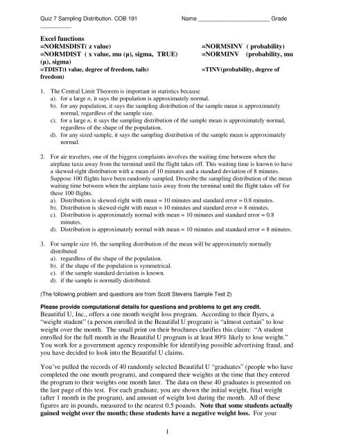
Quiz 7 Sampling Distribution. COB 191 Name _______________________ Grade
__________
Excel functions
=NORMSDIST( z value) =NORMSINV ( probability)
=NORMDIST ( x value, mu (µ), sigma, TRUE) =NORMINV (probability, mu
(µ), sigma)
=TDIST(t value, degree of freedom, tails) =TINV(probability, degree of
freedom)
1. The Central Limit Theorem is important in statistics because
a). for a large n, it says the population is approximately normal.
b). for any population, it says the sampling distribution of the sample mean is approximately
normal, regardless of the sample size.
c). for a large n, it says the sampling distribution of the sample mean is approximately normal,
regardless of the shape of the population.
d). for any sized sample, it says the sampling distribution of the sample mean is approximately
normal.
2. For air travelers, one of the biggest complaints involves the waiting time between when the
airplane taxis away from the terminal until the flight takes off. This waiting time is known to have
a skewed-right distribution with a mean of 10 minutes and a standard deviation of 8 minutes.
Suppose 100 flights have been randomly sampled. Describe the sampling distribution of the mean
waiting time between when the airplane taxis away from the terminal until the flight takes off for
these 100 flights.
a). Distribution is skewed-right with mean = 10 minutes and standard error = 0.8 minutes.
b). Distribution is skewed-right with mean = 10 minutes and standard error = 8 minutes.
c). Distribution is approximately normal with mean = 10 minutes and standard error = 0.8
minutes.
d). Distribution is approximately normal with mean = 10 minutes and standard error = 8 minutes.
3. For sample size 16, the sampling distribution of the mean will be approximately normally
distributed
a). regardless of the shape of the population.
b). if the shape of the population is symmetrical.
c). if the sample standard deviation is known.
d). if the sample is normally distributed.
(The following problem and questions are from Scott Stevens Sample Test 2)
Please provide computational details for questions and problems to get any credit.
Beautiful U, Inc., offers a one month weight loss program. According to their flyers, a
“weight student” (a person enrolled in the Beautiful U program) is “almost certain” to lose
weight over the month. The small print on their brochures clarifies this claim: “A student
enrolled for the full month in the Beautiful U program is at least 80% likely to lose weight.”
You work for a government agency responsible for identifying possible advertising fraud, and
you have decided to look into the Beautiful U claims.
You’ve pulled the records of 40 randomly selected Beautiful U “graduates” (people who have
completed the one month program), and compared their weights at the time that they entered
the program to their weights one month later. The data on these 40 graduates is presented on
the last page of this test. For each graduate, you are shown the initial weight, final weight
(after 1 month in the program), and amount of weight lost during the month. All of these
figures are in pounds, measured to the nearest 0.5 pounds. Note that some students actually
gained weight over the month; these students have a negative weight loss. For your
1

convenience, there is also a column recording whether a student lost weight (0 = “no weight
lost”, 1 = “some weight lost”).
The pulled records reveal that only 24 on the 40 graduates achieved any weight loss during
the month. That means that only 60% of the records pulled demonstrate any weight loss. The
question you must now consider is: is this evidence strong enough to justify an accusation of
false advertising by Beautiful U?
THE QUESTION:
Suppose that the average weight lost by a student in the program is 5 pounds, with a
standard deviation of 20 pounds. How likely is it that the average weight loss in a
random sample of 40 students will be 8.45 pounds or more?
4. Our task to find the probability that something is greater than or equal to 8.45. What is that “something”?
a) z b) σ c) s d) µ e) x (x-bar)
5. Our sample size is 40, so we’ll be able to apply our 191 techniques to answer THE QUESTION. This is
because the histogram of a 40 student sample suggests that the population is
a) perfectly normal b) roughly normal c) roughly symmetric d) roughly binomial e) bimodal
6. Question #2 says that “we’ll be able to apply our 191 techniques to answer THE QUESTION”. This is
because the observation that we made in Question #2 allows us to conclude that
a). the population is approximately normal
b). µ is approximately normal
c). the sampling distribution of the mean is approximately normal
d). s is a good approximation for σ
e). µ is a good approximation for x .
7. To answer THE QUESTION, we need to find
the standard deviation of the sampling
distribution of the mean. It is equal to
a). 20
b). 20/40 = 0.5
c). (8.45 - 5)/20 = 0.1725
d). SQRT(8.45 × (20 – 8.45)/40) = 1.562
e). 20/SQRT(40) = 3.162
2
8. We also need to know the mean of the
sampling distribution of the mean. In this
problem, this is
a). =NORMSINV(0.1725) = -0.9443
b). =NORMSINV(1-0.1725) = 0.9443
c). 5
d). =SQRT(40) = 6.325
e). 8.45
9. Which calculation would give the probability that one student chosen at random from the Beautiful U
graduates would have lost 8.45 pounds or more? (Assume, for this problem only, that weight loss is
normally distributed.)
a). = NORMDIST( 5, 8.45, 20, TRUE)
b). = NORMDIST( 5, 8.45, 3.162, TRUE)
c). = NORMDIST( 8.45, 5, 20, TRUE)
d). =1 - NORMDIST( 8.45, 5, 20, TRUE)
e). =1 - NORMDIST( 8.45, 5, 3.162, TRUE)
10. Suppose that the answer to THE QUESTION is 0.1376. What does this mean?
a). About 14% of all Beautiful U students lose 5 pounds or more.
b). About 14% of all Beautiful U students lose 8.45 pounds or more.
c). About 14% of the students in a sample of 40 students would be expected to lose 5 pounds or more.
d). About 14% of the students in a sample of 40 students would be expected to lose 8.45 pounds or more.
e). None of these interpretations is correct.

11. Suppose that the answer to THE QUESTION is 0.1376. Use this information to answer this question: How
likely is it that the average weight loss in a random sample of 40 Beautiful U students is between 1.55
pounds and 5 pounds? (Hint: Note that 1.55 + 3.45 = 5, and that 5 + 3.45 = 8.45. Draw a picture.)
i. a) About 14%. b) About 21% c) About 29% d) About 36% e) About 86%
12. Use the excerpt from Table E.2b appearing on the last page of this test to compute
P(-0.23 < z < 0.58). Its value is
i. a) 0.2888 b) 0.310 0 c) 0.690 0 d) 0.7112 e) 1.128
13. Consider these Excel expressions:
i. =NORMSINV(NORMSDIST(2))
ii. =NORMSDIST(NORMSINV(2)).
iii. Which of the following statements is true about the values that Excel assigns to these expressions?
(You may wish to draw a picture.)
iv. both expressions equal 2.
v. I equals 2, II is undefined.
vi. I is undefined, II equals 2.
vii. both expressions are undefined.
viii. the expressions are equal, but the value is probably not 2.
14. Consider these Excel expressions:
i. =NORMSINV(0.3)
ii. =NORMSINV(0.7).
Which of the following statements is true about the values that Excel assigns to these expressions?
(Hint: draw a picture.)
a). both expressions give the same value (i.e., I = II)
b). the value assigned to the two expressions add to one (i.e., I + II = 1)
c). the value assigned to the second expression is the negative of the value assigned to the first (i.e., II = -
I).
d). The difference of the two values would equal =NORMSINV(0.4)
e). (i.e., II – I = NORMSINV(0.4))
f). The difference of the two values would equal =NORMSINV(0.5) (i.e., II – I = NORMSINV(0.5))
15. Which of the following Excel expressions would give exactly the same value as =NORMSDIST(0.6)?
a). =NORMDIST(0.6, 1, 0, TRUE)
b). =NORMDIST(0.6, 0, 1, TRUE)
c). =NORMDIST(0.6, 1, 1, TRUE)
3
d) =NORMDIST(0.6, 1, 0,
FALSE)
e) =NORMSINV(0.4)

Weight
before
program
weight after
program
lost
weight?
weight
loss
189.5 198.0 0 -8.5
186 208.0 0 -22.0
175.5 176.0 0 -0.5
210 174.0 1 36.0
182 156.5 1 25.5
178 172.5 1 5.5
214 188.5 1 25.5
196 158.0 1 38.0
160 155.5 1 4.5
184 191.5 0 -7.5
184.5 148.5 1 36.0
171.5 123.0 1 48.5
176.5 151.5 1 25.0
160.5 169.0 0 -8.5
161.5 138.0 1 23.5
188 177.0 1 11.0
180.5 153.0 1 27.5
198 192.0 1 6.0
175 180.5 0 -5.5
175.5 179.0 0 -3.5
171 168.5 1 2.5
170 181.0 0 -11.0
165.5 139.5 1 26.0
192 189.5 1 2.5
157 165.5 0 -8.5
185.5 175.0 1 10.5
183 192.0 0 -9.0
213.5 187.5 1 26.0
162 189.5 0 -27.5
207 209.5 0 -2.5
184 162.5 1 21.5
221.5 239.0 0 -17.5
163.5 157.5 1 6.0
158 176.5 0 -18.5
158.5 179.0 0 -20.5
230.5 219.5 1 11.0
165 137.5 1 27.5
177 178.5 0 -1.5
171.5 138.5 1 33.0
174.5 143.0 1 31.5
average loss= 8.45 pounds
# losing wt = 24 students
# of graduates
12
10
8
6
4
2
0
z 0.00 0.01 0.02 0.03 0.04 0.05 0.06 0.07 0.08 0.09
-0.5 0.3085 0.3050 0.3015 0.2981 0.2946 0.2912 0.2877 0.2843 0.2810 0.2776
-0.4 0.3446 0.3409 0.3372 0.3336 0.3300 0.3264 0.3228 0.3192 0.3156 0.3121
-0.3 0.3821 0.3783 0.3745 0.3707 0.3669 0.3632 0.3594 0.3557 0.3520 0.3483
-0.2 0.4207 0.4168 0.4129 0.4090 0.4052 0.4013 0.3974 0.3936 0.3897 0.3859
-0.1 0.4602 0.4562 0.4522 0.4483 0.4443 0.4404 0.4364 0.4325 0.4286 0.4247
0 0.5000 0.5040 0.5080 0.5120 0.5160 0.5199 0.5239 0.5279 0.5319 0.5359
0.1 0.5398 0.5438 0.5478 0.5517 0.5557 0.5596 0.5636 0.5675 0.5714 0.5753
0.2 0.5793 0.5832 0.5871 0.5910 0.5948 0.5987 0.6026 0.6064 0.6103 0.6141
0.3 0.6179 0.6217 0.6255 0.6293 0.6331 0.6368 0.6406 0.6443 0.6480 0.6517
0.4 0.6554 0.6591 0.6628 0.6664 0.6700 0.6736 0.6772 0.6808 0.6844 0.6879
0.5 0.6915 0.6950 0.6985 0.7019 0.7054 0.7088 0.7123 0.7157 0.7190 0.7224
Entry represents area under the cumulative standardized normal distribution from -infinity to Z
4
-30 to
-20-
Weight Loss of 40 Graduates
-20 to
-10-
-10 to
0-
0 to
10-
10 to
20-
# of pounds lost
20 to
30-
30 to
40-
40 to
50-