by Milton Harris and Artur Raviv - Faculty
by Milton Harris and Artur Raviv - Faculty
by Milton Harris and Artur Raviv - Faculty

You also want an ePaper? Increase the reach of your titles
YUMPU automatically turns print PDFs into web optimized ePapers that Google loves.
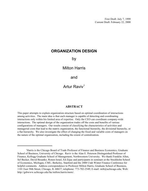
ORGANIZATION DESIGN<br />
<strong>by</strong><br />
<strong>Milton</strong> <strong>Harris</strong><br />
<strong>and</strong><br />
<strong>Artur</strong> <strong>Raviv</strong> 1<br />
ABSTRACT<br />
First Draft: July 7, 1999<br />
Current Draft: February 22, 2000<br />
This paper attempts to explain organization structure based on optimal coordination of interactions<br />
among activities. The main idea is that each manager is capable of detecting <strong>and</strong> coordinating<br />
interactions only within his limited area of expertise. Only the CEO can coordinate company-wide<br />
interactions. The optimal design of the organization trades off the costs <strong>and</strong> benefits of various<br />
configurations of managers. Our results consist of classifying the characteristics of activities <strong>and</strong><br />
managerial costs that lead to the matrix organization, the functional hierarchy, the divisional hierarchy, or<br />
a flat hierarchy. We also investigate the effect of changing the fixed <strong>and</strong> variable costs of managers on<br />
the nature of the optimal organization, including the extent of centralization.<br />
1 <strong>Harris</strong> is the Chicago Board of Trade Professor of Finance <strong>and</strong> Business Economics, Graduate<br />
School of Business, University of Chicago. <strong>Raviv</strong> is the Alan E. Peterson Distinguished Professor of<br />
Finance, Kellogg Graduate School of Management, Northwestern University. We thank Franklin Allen,<br />
Sel Becker, David Besanko, Ronen Israel, Ed Zajac <strong>and</strong> participants in seminars at the Stockholm School<br />
of Economics, Michigan, CMU, Berkeley, Stanford <strong>and</strong> the 2000 Utah Winter Finance Conference for<br />
helpful comments. Address correspondence to Professor <strong>Milton</strong> <strong>Harris</strong>, Graduate School of Business,<br />
1101 East 58th Street, Chicago, IL 60637; telephone: 773-702-2549; E-mail: milt@uchicago.edu; Web:<br />
http://gsbwww.uchicago.edu/fac/milton.harris/more/.
Organization Design<br />
<strong>by</strong> <strong>Milton</strong> <strong>Harris</strong> <strong>and</strong> <strong>Artur</strong> <strong>Raviv</strong><br />
Organizations are observed to exist with various structures. Many organizations are designed as<br />
hierarchies with each manager reporting to one <strong>and</strong> only one manager at the next higher level. Other<br />
organizations employ a matrix structure in which each low level manager reports to two or more<br />
superiors.<br />
Within the hierarchical structure, there is considerable variation in the number of levels <strong>and</strong> in<br />
the set of activities grouped together. The two main groupings are “divisional” <strong>and</strong> “functional.” In a<br />
divisional hierarchy, all the activities pertaining to a single product (or perhaps set of products) are<br />
grouped together into a division. For example, until the late 1980s Procter <strong>and</strong> Gamble (P & G) had a<br />
relatively flat hierarchical structure with only two levels. At the lower level were the br<strong>and</strong> managers.<br />
“Each br<strong>and</strong> – such as Tide, Crisco, Head <strong>and</strong> Shoulders <strong>and</strong> Scope – had its own br<strong>and</strong> manager who<br />
was singularly accountable for his or her br<strong>and</strong>’s performance.” [Robbins (1990, p. 295)]. The only<br />
other layer was headquarters. P & G then introduced a layer in between the br<strong>and</strong> managers <strong>and</strong><br />
headquarters. This layer contains division managers for product categories, such as laundry detergents,<br />
each responsible for advertising, sales, production, research, etc. for the br<strong>and</strong>s in his or her category. In<br />
a functional hierarchy, <strong>by</strong> contrast, activities pertaining to a particular function are organized into<br />
departments. For example, at Maytag, these departments include R & D, manufacturing, marketing,<br />
corporate planning, personnel, finance, labor relations, <strong>and</strong> legal [see Robbins (1990, pp. 286-87)]. In a<br />
functional hierarchy, the marketing department would, for example, coordinate marketing activities for<br />
all products.<br />
Matrix structure, which involves “dual-authority relations” [Jennergren (1981, p. 43)] can<br />
combine divisional <strong>and</strong> functional structures. For example, the manager in charge of design for project A<br />
D:\Userdata\Research\Hierarchies\temp.wpd 1 February 22, 2000 (11:18AM)
eports both to the Project A division manager <strong>and</strong> to the head of the design engineering group. In<br />
another example of the matrix form, the president of a unit producing power transformers in Norway for<br />
Asea Brown Boveri (ABB) reports to the president of ABB Norway <strong>and</strong> to the head of the Power<br />
Transformer Business Area [see Baron <strong>and</strong> Besanko (1997, p. 2)].<br />
To clarify the various ways firms are typically organized, consider the following hypothetical<br />
example. ABC Company produces <strong>and</strong> sells two versions of a product in two countries, Norway <strong>and</strong> the<br />
U.S. Each version of the product requires occasional country-specific design adaptations, <strong>and</strong>, of course,<br />
each version must be marketed in each country. There are thus four basic tasks, design <strong>and</strong> marketing for<br />
each version of the product. These four activities may be organized in one of four commonly observed<br />
structures, depicted in Figure 1-Figure 4. In Figure 1, the structure is flat with the manager in charge of<br />
each activity reporting directly to the CEO. Figure 2 depicts a divisional hierarchy in which there are<br />
two mid-level managers, each coordinating the two functions for a given country (product). In Figure 3,<br />
the hierarchy is organized along functional lines, i.e., each of the two middle managers is in charge of a<br />
function for both countries (products). Finally, Figure 4 shows a matrix organization in which each<br />
bottom level manager reports to two middle managers, e.g., the marketing manager for Norway reports<br />
both to the middle manager in charge of Norway <strong>and</strong> the middle manager in charge of global marketing.<br />
Figure 1: Flat Structure<br />
D:\Userdata\Research\Hierarchies\temp.wpd 2 February 22, 2000 (11:18AM)
Figure 2: Divisional Hierarchy<br />
Figure 3: Functional Hierarchy<br />
D:\Userdata\Research\Hierarchies\temp.wpd 3 February 22, 2000 (11:18AM)
CEO<br />
President,<br />
ABC<br />
Norway<br />
President,<br />
ABC US<br />
Chief,<br />
Global<br />
Marketing<br />
Head,<br />
Norway<br />
Marketing<br />
Head,<br />
US<br />
Marketing<br />
Figure 4: Matrix Organization<br />
Chief,<br />
Design<br />
Head,<br />
Norway<br />
Design<br />
Head,<br />
US<br />
Design<br />
An interesting topic in the theory of the firm, relatively under explored in the economics<br />
literature, is what determines whether an organization adopts a matrix or hierarchical structure, how<br />
many levels are involved <strong>and</strong> how activities are grouped. Several authors in the organization behavior<br />
literature have argued that the choice between divisional <strong>and</strong> functional structures is driven <strong>by</strong> the<br />
relative importance of coordination of functional activities within a product line <strong>and</strong> economies of scale<br />
from combining similar functions across product lines. 2 The advantage of a divisional structure is that it<br />
allows better coordination among the various functions, such as manufacturing, product design,<br />
personnel, <strong>and</strong> marketing, required to produce <strong>and</strong> sell a product. Segregating these functions <strong>by</strong> product<br />
divisions, however, results in the failure to exploit economies of scale available if, for example,<br />
marketing for all products is h<strong>and</strong>led <strong>by</strong> a central marketing department. Trading off these advantages, it<br />
2 See the survey <strong>by</strong> Jennergren (1981) for a summary of this literature.<br />
D:\Userdata\Research\Hierarchies\temp.wpd 4 February 22, 2000 (11:18AM)
is argued, determines whether one adopts a divisional or a functional hierarchy.<br />
We address the issues relating to organization design mentioned above using a model based on<br />
coordinating interactions across various activities. In our view, coordinating interactions requires costly<br />
expertise embodied in managers. The optimal organizational structure trades off the benefits of<br />
coordination against the cost of the necessary expertise. In this sense it is similar to the arguments of<br />
organization theorists summarized in the previous paragraph. We provide a formal model that extends<br />
the ideas beyond the functional vs. divisional choice. The model endogenizes the choice of organization<br />
structure allowing us to make predictions regarding the use of matrix vs. hierarchical structures <strong>and</strong> the<br />
extent of decentralization. If a hierarchy is used, we rationalize the choice of functional vs. divisional<br />
grouping <strong>and</strong> vertical span.<br />
We model a firm as consisting of activities such as producing products or components, designing<br />
products, marketing products, etc. Each activity originates with a “project manager” who is assumed to<br />
be essential to generating the activity <strong>and</strong> to have no function other than generating <strong>and</strong> possibly<br />
managing his activity. If a set of activities interacts, there are benefits to coordinating these activities.<br />
Reaping these benefits requires coordination <strong>by</strong> a manager with the correct expertise (project managers<br />
have no coordination expertise). The territory between the project managers <strong>and</strong> the CEO, may be<br />
populated <strong>by</strong> various “middle managers.” Each middle manager is capable of detecting <strong>and</strong> coordinating<br />
a specific pair of interactions. In addition to the benefits of coordinating pairs of activities, there are<br />
incremental benefits to coordinating a set of activities on a company-wide basis. Only the CEO is<br />
capable of this company-wide coordination (the CEO can also coordinate pairs of activities <strong>and</strong> may<br />
engage in other, unmodeled activities). It is important to note that we abstract entirely from incentive<br />
problems. That is, in our model, managers act in the best interest of shareholders <strong>and</strong> have no incentive<br />
to hide or distort information that they discover. We return to this issue briefly in the concluding section.<br />
These managers may have both fixed <strong>and</strong> variable costs. The fixed cost of a manager must be<br />
D:\Userdata\Research\Hierarchies\temp.wpd 5 February 22, 2000 (11:18AM)
paid if the manager is available to coordinate activities for the firm, regardless of whether that manager is<br />
actually used. A manager’s variable cost is paid only if the manager’s expertise is actually used to<br />
coordinate activities. This is an opportunity cost of the manager’s time that is related to his value in<br />
other activities not modeled here. For example, the variable cost of a CEO might be related to her value<br />
in strategic planning.<br />
The organization design problem is to choose a set of middle managers who are available for<br />
coordinating activities <strong>and</strong> a set of instructions for using these managers, the project managers <strong>and</strong> the<br />
CEO, given the costs of having <strong>and</strong> using these managers <strong>and</strong> the expected coordination benefits. Our<br />
results consist of classifying the characteristics of activities <strong>and</strong> managerial costs that lead to various<br />
structures. When the fixed cost of middle managers is high, no middle managers are employed, <strong>and</strong> the<br />
resulting structure is a flat organization consisting only of the CEO <strong>and</strong> the project managers. When the<br />
middle managers’ fixed cost is low, the resulting structure resembles a matrix form rich in middle<br />
managers. For intermediate fixed costs of the middle managers, a hierarchy with some middle managers<br />
is optimal. Increases in the variable cost of the CEO may also result in employing more middle managers<br />
as well as reducing the involvement of the CEO in coordination activities, i.e., reducing the centralization<br />
of decision making. Also, increases in the synergy gains from coordinating company-wide interactions<br />
increase centralization.<br />
It is not surprising that increases in the fixed cost of middle managers lead to reduction in their<br />
employment or that increases in synergy gains or reductions in CEO variable cost lead to greater<br />
centralization. To underst<strong>and</strong> the intuition for the result that increases in the variable cost of the CEO<br />
lead to more middle-management-intensive structures, it is helpful first to realize that the middle<br />
managers have two functions in our model. One is to coordinate pairs of projects when they interact.<br />
The other is to generate information that allows more efficient use of the CEO, i.e., to protect the CEO.<br />
In particular, middle managers allow a more accurate assessment of whether a company-wide interaction<br />
D:\Userdata\Research\Hierarchies\temp.wpd 6 February 22, 2000 (11:18AM)
is present. This information enables the firm to reap the benefits of company-wide coordination in some<br />
situations when it would otherwise be suboptimal. It also allows the firm to avoid wasting the CEO’s<br />
time when the company-wide interaction is unlikely to be present. Consequently, as the cost of the<br />
CEO’s time in coordination activities increases, middle managers become more valuable in their function<br />
as protectors of the CEO.<br />
A number of empirical implications follow from these results. Under certain additional<br />
assumptions, we show that organization structure will exhibit a sort of “life cycle” as the organization<br />
grows in complexity <strong>and</strong> size. In particular, we show that the structure will progress from a flat, but<br />
highly centralized structure, to a divisional hierarchy to a functional hierarchy <strong>and</strong> then either to a matrix<br />
structure or to a flat, highly decentralized structure. We also show that conglomerates that are organized<br />
as hierarchies may be expected to exhibit divisional, as opposed to functional, hierarchies. Finally, we<br />
show that firms that do not face tight resource constraints, highly regulated firms, <strong>and</strong> firms in stable<br />
environments will tend to have decentralized organizational structures.<br />
The remainder of the paper is organized as follows. A brief review of the literature is contained<br />
in the next section. The model is presented formally in Section 2. We then solve the problem of how to<br />
use a given set of middle managers in Section 3. This results in an optimal value (i.e., coordination<br />
benefits net of costs) for each set of middle managers. These values are compared to obtain an overall<br />
best design in Section 4. Comparative statics results are presented in Section 5, empirical implications<br />
are considered in Section 6, <strong>and</strong> conclusions are presented in Section 7.<br />
1 Literature Review<br />
The economics literature on organization design is, as mentioned above, somewhat sparse. One<br />
approach, adopted <strong>by</strong> Radner (1993), is to assume that processing information takes valuable time. To<br />
reduce the delay, one can use “parallel processing” involving several people processing part of the<br />
D:\Userdata\Research\Hierarchies\temp.wpd 7 February 22, 2000 (11:18AM)
information at the same time. Delay reduction can be traded off against the cost of more “processors.”<br />
Generally, this does not result in the types of organization structures we usually observe. Bolton <strong>and</strong><br />
Dewatripont (1994) have a similar approach but emphasize the tradeoff between specialization <strong>and</strong><br />
communication. They show that in most cases, the optimal organization structure combines a hierarchy<br />
with a “conveyer belt” type of structure. Sah <strong>and</strong> Stiglitz (1986) also focus on sequential vs. parallel<br />
processing of information but investigate the tradeoff between type I <strong>and</strong> type II errors to determine when<br />
sequential processing is better than parallel processing <strong>and</strong> vice versa.<br />
Garicano (1997) provides an elegant theory of hierarchies, based on expertise, that is similar in<br />
some respects to ours. He postulates the presence of experts who can be ranked according to the<br />
difficulty of the problems they can solve. Experts in a given cohort can solve all problems that can be<br />
solved <strong>by</strong> those in lower cohorts plus some more difficult problems. Experts who can solve more<br />
problems are correspondingly more expensive. More difficult problems occur less frequently than less<br />
difficult ones, however. This results in a pyramidical hierarchy with more workers at lower levels <strong>and</strong><br />
fewer at higher levels. In analyzing hierarchies, we more-or-less assume a pyramidical structure but<br />
allow contingent referral of projects. We also consider experts with non-nested expertise allowing for<br />
the optimality of matrix forms.<br />
Hart <strong>and</strong> Moore (1999) provide a model of hierarchies based on authority over the<br />
implementation of ideas for using assets. In their model, if individual i has authority over individual j<br />
with respect to ideas for a set of assets, then j’s idea for those assets will be implemented if <strong>and</strong> only if i<br />
has no idea. The issue is how best to assign identical individuals to sets of assets, i.e., to which assets to<br />
assign each individual <strong>and</strong> in which order (where order indicates authority). Hart <strong>and</strong> Moore distinguish<br />
between coordination activities, in which an individual is assigned to more than one asset, <strong>and</strong><br />
specialization activities, in which an individual is assigned to only one asset. To implement one’s idea<br />
for a set of assets, one must have the highest authority of those who have an idea for any asset in the set.<br />
D:\Userdata\Research\Hierarchies\temp.wpd 8 February 22, 2000 (11:18AM)
Hart <strong>and</strong> Moore show that if the probability of having an idea for a set of assets decreases as the size of<br />
the set increases <strong>and</strong> if sets of assets for which synergies exist are disjoint, then the optimal structure will<br />
involve a pyramidical hierarchy with individuals whose tasks cover a larger set of assets appearing higher<br />
in the chain of comm<strong>and</strong>. Although this model shares with ours the idea that coordination of activities is<br />
an important determinant of organization design, the approaches are quite different. The Hart-Moore<br />
model focuses on authority, whereas we focus on information. Their results explain authority relations<br />
(e.g., coordinators should be senior to specialists) but do not explain hierarchical groupings (functional<br />
vs. divisional) or matrix forms as we do. Hart <strong>and</strong> Moore relate the extent of centralization to the size of<br />
coordination benefits, whereas we focus on costs of expertise as the main determinants of centralization.<br />
Vayanos (1997) stresses the interaction of information, i.e., the idea that the best project in a<br />
subset may depend on the nature of projects outside that subset. This feature is absent from other models<br />
in the economics literature, e.g., Radner (1993), Bolton <strong>and</strong> Dewatripont (1994), <strong>and</strong> Garicano (1997),<br />
but is one we emphasize. The application Vayanos models is portfolio selection. He assumes a<br />
hierarchy in which managers at each level examine a set of portfolios suggested <strong>by</strong> subordinates <strong>and</strong> an<br />
exogenously determined set of assets (except the lowest level managers who examine only assets). Each<br />
manager chooses weights for combining these portfolios <strong>and</strong> assets into a larger portfolio (without<br />
changing the weights of the items in the submitted portfolios). Managers ignore assets outside their<br />
purview when choosing weights. The main result is that each agent in the hierarchy (except the lowest)<br />
has exactly one subordinate <strong>and</strong> also examines some assets directly. 3<br />
The organization behavior literature has investigated the empirical relationships between<br />
decentralization of decisions <strong>and</strong> such variables as size (measured <strong>by</strong> employment) <strong>and</strong> vertical<br />
integration. Blau <strong>and</strong> Schoenherr (1971), Child (1973), Donaldson <strong>and</strong> Warner (1974), Hinings <strong>and</strong> Lee<br />
3 Calvo <strong>and</strong> Wellisz (1979) also assume a hierarchical structure. Their main focus is explaining<br />
wage differentials across levels of the hierarchy.<br />
D:\Userdata\Research\Hierarchies\temp.wpd 9 February 22, 2000 (11:18AM)
(1971), Kh<strong>and</strong>walla (1974) <strong>and</strong> Pugh et al. (1969) all find a positive relationship between size <strong>and</strong> extent<br />
of decentralization. K<strong>and</strong>walla (1974) also documents a positive relationship between vertical<br />
integration <strong>and</strong> decentralization. Child (1973) finds that the vertical span (number of levels) of hierarchy<br />
is positively related to size.<br />
2 Model<br />
We model a firm that, for tractability, is assumed to engage in only four projects, labeled A, B,<br />
C, <strong>and</strong> D over a single period. Various subsets of these four projects may or may not interact. We<br />
denote an interaction between two projects <strong>by</strong> juxtaposing their labels, e.g., AB denotes an interaction<br />
between projects A <strong>and</strong> B. The set of feasible pairwise interactions is denoted <strong>by</strong> Ω = {AB,CD,AC,BD}.<br />
Note that we have excluded two interactions, i.e., AD <strong>and</strong> BC. This greatly simplifies the analysis <strong>and</strong><br />
reflects the idea that some interactions are a priori extremely unlikely. For example, the design of a<br />
product intended for sale in Norway <strong>and</strong> marketing of the U.S. version of the product are not likely to<br />
interact directly. Which of the feasible interactions occurs is given <strong>by</strong> an elementary event e @ Ω. That<br />
is, e is interpreted as the event that exactly those pairs of projects ω e interact <strong>and</strong> no others. Thus, for<br />
example, the event e = {AB,CD} indicates that projects A <strong>and</strong> B interact, projects C <strong>and</strong> D interact, <strong>and</strong><br />
no other projects interact. The event e = Ω indicates that all four possible interactions occurred. We<br />
refer to this event as a “company-wide” interaction. The event e = E indicates that no interaction has<br />
occurred. The set of elementary events is denoted <strong>by</strong> E = 2 Ω (the set of all subsets of Ω).<br />
To simplify the analysis <strong>and</strong> to capture the notion that some interactions tend to be similar to<br />
each other, we divide the set of feasible interactions, Ω, into two groups, P = {AB,CD} <strong>and</strong> R =<br />
{AC,BD}. For example, suppose A is production of Tide, B is marketing of Tide, C is production of<br />
Cheer, <strong>and</strong> D is marketing of Cheer. Then the above grouping reflects the assumption that interactions<br />
within a product line are similar to each other. We take similarity to the extreme <strong>by</strong> assuming the<br />
D:\Userdata\Research\Hierarchies\temp.wpd 10 February 22, 2000 (11:18AM)
interactions in a given group are identical in terms of probability of occurrence (later we assume that the<br />
benefits of coordinating these interactions are also the same). Formally, assume that the probability of<br />
either interaction in P is p, <strong>and</strong> the probability of either interaction in R is r. We also assume that<br />
interactions are independent, <strong>and</strong> these probabilities are observed <strong>by</strong> everyone in the firm. 4 We assume p<br />
> r, i.e, interactions between A <strong>and</strong> B <strong>and</strong> between C <strong>and</strong> D are the more likely interactions, while<br />
interactions between A <strong>and</strong> C <strong>and</strong> B <strong>and</strong> D are less likely. In terms of the above example, the assumption<br />
is that interactions within a product line are more likely than those across product lines. If, on the other<br />
h<strong>and</strong>, the economies of scale from combining production activities <strong>and</strong> those from combining marketing<br />
activities are more likely than interactions across functions within product lines, then we would simply<br />
relabel the activities so that A is production of Tide, B is production of Cheer, C is marketing of Tide,<br />
<strong>and</strong> D is marketing of Cheer.<br />
There are three types of potential managers, project managers (one for each project), middle<br />
managers, <strong>and</strong> a CEO. Project managers are required to generate the projects <strong>and</strong> participate in<br />
managing them but cannot coordinate interactions between projects. They do, however, refer projects to<br />
middle management or the CEO for investigation <strong>and</strong> coordination of possible interactions.<br />
If a set of projects does interact, there are benefits to coordinating them. Discovering <strong>and</strong><br />
reaping these benefits requires investigation <strong>and</strong> coordination <strong>by</strong> a middle manager with the correct<br />
expertise (or <strong>by</strong> the CEO). For each interaction ω Ω, a middle manager, denoted m ω, may be hired who<br />
can discover <strong>and</strong> coordinate this interaction <strong>and</strong> only this interaction. The set of potentially available<br />
middle managers is denoted <strong>by</strong> M = {m ω�ω Ω}. We can think of the middle managers in M as product<br />
division managers, managers of functional areas (e.g., marketing manager), country managers, etc.,<br />
depending on the interpretation of the activities A, B, C, <strong>and</strong> D. Let M P (M R) denote the set of middle<br />
4 As was pointed out in the Introduction, we abstract from all private information <strong>and</strong> incentive<br />
problems. While these may also be important determinants of organization structure [see Qian (1994),<br />
Singh (1985)], we limit the scope of the current paper to a consideration of coordination issues.<br />
D:\Userdata\Research\Hierarchies\temp.wpd 11 February 22, 2000 (11:18AM)
managers who can discover <strong>and</strong> coordinate interactions in P (respectively, R), i.e.,<br />
M P = {m ω�ω P} <strong>and</strong> M R = {m ω�ω R}.<br />
Incremental benefits from coordinating the pairwise interactions are assumed to be the same for all pairs<br />
<strong>and</strong> are normalized to one. Thus, the probabilities p <strong>and</strong> r also play the role of expected benefits of the<br />
potential interactions.<br />
The CEO, denoted m*, is assumed to be able to discover <strong>and</strong> exploit any interaction, but only the<br />
CEO can exploit the company-wide interaction which is assumed to be present if all four pairwise<br />
interactions occur. Incremental benefits from coordinating the company-wide interaction are given <strong>by</strong> s. 5<br />
Incremental benefits produced <strong>by</strong> the CEO depend on which benefits, if any, middle managers have<br />
already exploited. In particular, m* generates benefits of 1 for each interaction present but not exploited<br />
<strong>by</strong> a middle manager plus s if all four pairwise interactions are present.<br />
This formalism admits many possible interpretations. For example, A <strong>and</strong> C can be electrical<br />
devices in Chevies <strong>and</strong> Cadillacs, respectively, <strong>and</strong> B <strong>and</strong> D can be chassis of Chevies <strong>and</strong> Cadillacs,<br />
respectively. If project A turns out to be headlight improvement <strong>and</strong> B crash resistance, then A <strong>and</strong> B are<br />
likely to interact in that both improve the safety of Chevies. If they do interact, exploiting this interaction<br />
through a coordinated marketing effort emphasizing safety will produce incremental benefits. If,<br />
however, B is roominess, then A <strong>and</strong> B are unlikely to interact. One can interpret m AB (m CD) as the<br />
manager of the Chevy (Cadillac) Division <strong>and</strong> m AC (m BD) as the head of electronics (chassis).<br />
An alternative interpretation is that A <strong>and</strong> B are innovations in products 1 <strong>and</strong> 2, respectively,<br />
while C <strong>and</strong> D are new marketing techniques for the two products, respectively. The innovations may<br />
have common components calling for coordinated production. The new marketing techniques may call<br />
for a common ad campaign for the two products. One can interpret m AB (m CD) as the manager of the<br />
5 One role of the CEO in an organization may be to resolve conflicts in coordinating between two<br />
or more interactions involving the same project, e.g., between AB <strong>and</strong> AC. One can interpret s in our<br />
model as the benefit to such conflict resolution.<br />
D:\Userdata\Research\Hierarchies\temp.wpd 12 February 22, 2000 (11:18AM)
Production (Marketing) Division <strong>and</strong> m AC (m BD) as the manager of the Product 1 (2) Division.<br />
As mentioned in the Introduction, managers have both fixed <strong>and</strong> variable costs. The fixed cost is<br />
a cost associated with employing the manager whether that manager is actually used to coordinate any<br />
projects. Empirically, we identify the manager’s fixed cost with his salary. A manager’s variable cost is<br />
an opportunity cost of the manager’s time that is related to his value in other activities not modeled here.<br />
Since project managers are assumed to be essential to generating projects <strong>and</strong> to have no function<br />
other than generating <strong>and</strong> possibly managing projects, the cost (both fixed <strong>and</strong> variable) of project<br />
managers can be ignored. For simplicity, we assume that all middle managers have the same fixed cost,<br />
denoted F <strong>and</strong> that the middle managers have no function other than discovering <strong>and</strong> coordinating<br />
interactions between projects. Therefore, the variable cost of the middle managers is zero. The CEO,<br />
however, is assumed to have other duties such as strategic planning. Consequently the CEO’s variable<br />
cost is positive <strong>and</strong> is denoted <strong>by</strong> Q. These other duties of the CEO are sufficiently valuable that the<br />
CEO is required. Consequently, her fixed cost can be ignored. We further simplify the problem (<strong>and</strong><br />
eliminate some uninteresting cases) <strong>by</strong> assuming that the value added <strong>by</strong> the CEO in coordinating the<br />
company-wide interaction exceeds her variable cost, i.e.,<br />
Assumption 1. s > Q.<br />
3 Optimal Use of a Given Set of Middle Managers<br />
We find an optimal organization design in two stages. In this section, for each possible subset of<br />
available middle managers, we optimize their use <strong>and</strong> calculate the expected net benefits associated with<br />
this program. The overall organization design problem can then be solved <strong>by</strong> comparing these expected<br />
net benefits. This is done in Section 4.<br />
Given the available middle managers <strong>and</strong> the project characteristics, p <strong>and</strong> r, the problem is to<br />
decide which managers should be used to check for <strong>and</strong> coordinate possible interactions <strong>and</strong> in what<br />
D:\Userdata\Research\Hierarchies\temp.wpd 13 February 22, 2000 (11:18AM)
order <strong>and</strong> in which contingencies they should be used. The problem is vastly simplified, however, <strong>by</strong> the<br />
assumption that the middle managers have no variable costs. It follows that it is optimal to use any<br />
middle managers that are available.<br />
In the next three subsections, we analyze in turn the cases of no middle managers, two middle<br />
managers, <strong>and</strong> all four middle managers, respectively.<br />
3.1 No Middle Managers: Centralized <strong>and</strong> Decentralized Flat Structure<br />
When no middle managers are employed (i.e., the structure is flat), the problem is simply to<br />
decide whether to refer all four projects to the CEO or to give up any coordination benefits <strong>and</strong> let the<br />
project managers run the projects. We refer to the flat structure when all projects are referred to the CEO<br />
as the centralized flat structure. The expected benefit of this structure is the expected benefit from<br />
coordinating the four pairwise interactions, p+p+r+r, plus the synergy gain, s, from the company-wide<br />
interaction times the probability of the company-wide interaction, p 2 r 2 . The cost of referring projects to<br />
the CEO is her opportunity cost, Q. Therefore, expected net profit for the centralized flat structure is<br />
2(p+r)+p 2 r 2 s Q. We refer to the flat structure when no projects are referred to the CEO as the<br />
decentralized flat structure. In this case, there are no coordination benefits <strong>and</strong> also no costs, so the<br />
expected net profit is zero. Therefore, the net value of the flat structure is<br />
3.2 Two Middle Managers: Hierarchies<br />
V F max$2(p r) p 2 r 2 s Q,0�. (1)<br />
In this subsection we consider the problem assuming that only two middle managers are<br />
available. Since interactions are identical within a group, either P or R, there are only two relevant cases:<br />
only managers in M R are available or only those in M P are available. 6 We consider, for each case, the<br />
6 There is one other possibility, namely employing one manager from each of MP <strong>and</strong> M R. This<br />
structure does not, however, resemble a hierarchy (since one project will be referred to two middle<br />
managers) or any other commonly observed organizational forms. Consequently, we rule out this<br />
D:\Userdata\Research\Hierarchies\temp.wpd 14 February 22, 2000 (11:18AM)
optimal use of the given two managers.<br />
possibility.<br />
When only managers from M R or only those from M P are available, the structure resembles a<br />
hierarchy in which each project is referred (at most) to one <strong>and</strong> only one manager at the next level. For<br />
example, if only managers from M P are available, projects A <strong>and</strong> B are referred to m AB <strong>and</strong> projects C<br />
<strong>and</strong> D are referred to m CD. Consequently, we refer to these two situations as the R-hierarchy <strong>and</strong> the P-<br />
hierarchy, respectively.<br />
First suppose only managers in M R are present. To calculate the value of an optimal strategy in<br />
this case, we use backward induction. Suppose projects have been referred to the two managers in M R.<br />
At this point one may either stop or refer all projects to the CEO. In the former case, the middle<br />
managers coordinate their interactions, <strong>and</strong> the CEO is not involved. Consequently, we refer to this case<br />
as the decentralized R-hierarchy. In the latter case, the middle managers coordinate their interactions,<br />
while the CEO coordinates the other pairwise interactions <strong>and</strong> the company-wide interaction.<br />
Accordingly, we refer to this case as the centralized R-hierarchy. Stopping results in a net additional<br />
expected benefit of zero. Referring projects to the CEO results in a net additional expected benefit that<br />
depends on whether the two managers in M R both found interactions. If both interactions are found (this<br />
happens with probability r 2 ), the additional expected benefit of referring all projects to the CEO consists<br />
of the expected coordination benefits for the two projects in P, 2p, <strong>and</strong> the expected company-wide<br />
synergy gain, p 2 s. The cost of referring to the CEO is Q, so the expected net benefit is 2p+p 2 s Q. If at<br />
least one of the interactions from the R group failed to occur (this happens with probability 1 r 2 ), the<br />
additional net benefit of referring all projects to the CEO is only 2p Q, since the company-wide<br />
interaction is not present in this case. Thus the expected value of an optimal continuation strategy, given<br />
that both managers from M R have been consulted, is r 2 max{2p+p 2 s Q,0}+(1 r 2 )max{2p Q,0}. The<br />
expected benefit from referring projects to the two middle managers is simply 2r. Therefore, the optimal<br />
D:\Userdata\Research\Hierarchies\temp.wpd 15 February 22, 2000 (11:18AM)
value of the R-hierarchy (net of fixed costs) is<br />
V R 2r r 2 max$2p p 2 s Q,0� (1 r 2 )max$2p Q,0� 2F. (2)<br />
By symmetry we have the following analogous value for a P-hierarchy: 7<br />
V P 2p p 2 max$2r r 2 s Q,0� (1 p 2 )max$2r Q,0� 2F. (3)<br />
3.3 Four Middle Managers: Matrix Structure<br />
As mentioned above, given that all four middle managers are present, it is optimal to have them<br />
investigate the four possible interactions first, before referring any decisions to the CEO. This strategy<br />
allows the firm to reap any benefits from interactions that are present <strong>and</strong> involve the CEO only if it is<br />
known that a company-wide interaction requiring her special expertise exists. The strategy corresponds<br />
to the matrix organization described in the Introduction. That is, each project manager refers his project<br />
to two upper level managers: project A is referred both to m AB <strong>and</strong> m AC, project B is referred both to m AB<br />
<strong>and</strong> m BD, etc.<br />
computed as<br />
Using Assumption 1, the value of the matrix organization net of fixed costs can easily be<br />
V M 2(p r) p 2 r 2 (s Q) 4F. (4)<br />
The intuition for this expression is as follows. Given that all four middle managers will be used <strong>and</strong> that,<br />
if the company-wide interaction occurs, projects are referred to the CEO, the expected benefit is the<br />
expected benefit from each single interaction, p+p+r+r, plus the expected value added of the CEO net of<br />
her variable cost, p 2 r 2 (s Q). The expected cost is the fixed cost of the four middle managers, 4F. The<br />
difference between the expected benefit <strong>and</strong> the expected cost gives the value of the matrix form in (4).<br />
7 Note that, for the R-hierarchy, if Q < 2p, then all projects will eventually be referred to the CEO<br />
no matter what is discovered <strong>by</strong> the middle managers. A similar statement holds for the P-hierarchy<br />
when Q < 2r. For either hierarchy, this is equivalent simply to referring all projects directly to the CEO,<br />
skipping the middle managers. In this case, hierarchies would clearly be suboptimal, since a hierarchy<br />
would provide the same benefit as the centralized flat structure but would cost 2F more. Consequently,<br />
in an optimal design, if a centralized hierarchy is used, it will be one in which the CEO is involved only<br />
if both middle managers find interactions.<br />
D:\Userdata\Research\Hierarchies\temp.wpd 16 February 22, 2000 (11:18AM)
We summarize the results of this section in Table 1 which shows, for various values of the<br />
opportunity cost Q of the CEO, the optimal value of each organization design. In constructing the table,<br />
we have made the following simplifying assumption.<br />
Assumption 2. r 2 (1 p 2 )s >2p.<br />
This assumption allows us to define six ranges for Q such that in each range, the max operator that<br />
appears in the formulas for the values of each design can be resolved. Assumption 2 is consistent with<br />
the spirit of Assumption 1, namely that the value added of the CEO in coordinating activities is large.<br />
For Q V F V R V P V M<br />
[0,2r)<br />
[2r,2p)<br />
[2p,G)<br />
[G,2r+r 2 s)<br />
[2r+r 2 s,2p+p 2 s)<br />
G Q<br />
D(Q) 2(p r) p 2r 2 (s Q),<br />
G 2(p r) p 2r 2s, Kxy (Q) 4x 2x 2 (2y y 2 In the above table, the symbols D, G, <strong>and</strong> K are defined <strong>by</strong><br />
s Q), for (x,y) $(p,r),(r,p)�.<br />
4 Optimal Organization Design<br />
Table 1: Value of Each Design as a Function of Q<br />
G Q 2F<br />
2F+K rp(Q)/2<br />
[2p+p 2 s,") 2r 2F<br />
The optimal organization design is found <strong>by</strong> comparing the values of the various designs. This<br />
comparison is most easily performed <strong>by</strong> row in Table 1.<br />
0<br />
G Q 2F<br />
2F+K pr(Q)/2<br />
2p 2F<br />
D(Q) 4F<br />
For very low opportunity cost of the CEO, Q < 2r, even if there is no company-wide interaction,<br />
D:\Userdata\Research\Hierarchies\temp.wpd 17 February 22, 2000 (11:18AM)
it is still optimal to use the CEO to discover <strong>and</strong> coordinate pairwise interactions. This fact has two<br />
important implications. First, it implies that, when using the flat structure, it is optimal to refer all<br />
projects to the CEO, i.e, use the centralized flat structure. Second, it also implies that, for either<br />
hierarchy, it is optimal to refer all projects to the CEO, regardless of what is found <strong>by</strong> the two middle<br />
managers. In this case, however, the cost, 2F, of the two middle managers is wasted, because the same<br />
result can be obtained from the flat structure with no middle managers <strong>by</strong> referring all projects directly to<br />
the CEO. Therefore, for Q < 2r, the optimal design is either the centralized flat structure or the matrix<br />
organization. In this range of Q, both designs exploit all interactions that are present. The advantage of<br />
the matrix is that the opportunity cost of the CEO is incurred only when it is known for sure that the<br />
company-wide interaction is present. That is, the matrix saves A(Q) � Q(1 p 2 r 2 ) on average relative to<br />
the flat structure. The disadvantage is, of course, the fixed cost of the four middle managers, 4F. Thus<br />
when this fixed cost is large relative to the CEO’s opportunity cost, the flat structure is preferred, i.e., the<br />
optimal design in this range of Q is the centralized flat structure when 4F > A(Q) <strong>and</strong> the matrix<br />
organization otherwise.<br />
For Q [2r,2p), the same argument as in the previous paragraph applies to the R-hierarchy, i.e.,<br />
in the R-hierarchy, it is optimal to refer all projects to the CEO, regardless of what is found <strong>by</strong> the two<br />
middle managers. This is not true for the P-hierarchy, because for that hierarchy the expected payoff of<br />
referring to the CEO in the absence of a company-wide interaction is only 2r < Q. Thus in this range of<br />
Q, the optimal design is either the centralized flat structure, the P-hierarchy, or the matrix organization.<br />
As before, the centralized flat structure dominates the matrix when 4F > A(Q). The advantages of the<br />
flat structure relative to the P-hierarchy are that it saves 2F in fixed costs of middle managers <strong>and</strong> it<br />
exploits all interactions that are present. The P-hierarchy refers projects to the CEO (it is centralized) but<br />
only when both of the high probability interactions are present. As a result, the centralized P-hierarchy<br />
saves Q(1 p 2 ) on average in CEO costs but forgoes benefits of 2r(1 p 2 ) on average relative to the flat<br />
D:\Userdata\Research\Hierarchies\temp.wpd 18 February 22, 2000 (11:18AM)
structure. Thus, the flat structure is better than the centralized P-hierarchy when 2F > (1 p 2 )(Q 2r) or<br />
4F > B pr(Q) �2(1 p 2 )(Q 2r). Consequently, for Q [2r,2p), the flat structure is optimal when 4F > A(Q)<br />
<strong>and</strong> 4F > B pr(Q).<br />
Obviously, the matrix organization is better than the flat structure in this range of Q when 4F <<br />
A(Q). Relative to the centralized P-hierarchy, the matrix saves the opportunity cost of the CEO when the<br />
two high-probability interactions are present, but the company-wide interaction is not, i.e., the matrix<br />
saves Q(p 2 p 2 r 2 ). The matrix also always exploits the low-probability interactions when present, while<br />
the centralized P-hierarchy exploits them only when the high-probability interactions are present. Thus<br />
the matrix produces additional expected benefits of 2r(1 p 2 ) relative to the centralized P-hierarchy. On<br />
the other h<strong>and</strong>, the matrix costs 2F more in middle manager fixed costs. Thus the matrix is better than<br />
the centralized P-hierarchy when 2F < Qp 2 (1 r 2 )+2r(1 p 2 ) or 4F < C pr(Q) � 2Qp 2 (1 r 2 )+4r(1 p 2 ).<br />
Consequently, for Q [2r,2p), the matrix organization is optimal when 4F < A(Q) <strong>and</strong> 4F < C pr(Q).<br />
When neither of the conditions in the previous two paragraphs is satisfied, i.e., when A(Q) < 4F<br />
< C pr(Q), the centralized P-hierarchy is optimal.<br />
For Q [2p,G), the comparisons between the flat structure, the matrix, <strong>and</strong> the P-hierarchy are<br />
the same as for Q [2r,2p). In this range of Q, however, the R-hierarchy becomes a viable alternative.<br />
The comparisons between the R-hierarchy <strong>and</strong> the flat <strong>and</strong> matrix structures are, however, the same as<br />
those between the P-hierarchy <strong>and</strong> the other two organizations except that the roles of p <strong>and</strong> r are<br />
reversed. Thus, the centralized flat structure is optimal when 4F > max{A(Q),B pr(Q),B rp(Q)}, the matrix<br />
organization is optimal when 4F < min{A(Q),C pr(Q),C rp(Q)}, <strong>and</strong> otherwise one of the hierarchies is<br />
optimal. To compare the two hierarchies, first, recall that the difference between them is which two<br />
middle managers are available for discovering <strong>and</strong> coordinating interactions. In the R-hierarchy, the<br />
managers who can analyze the low-probability interactions are available. In the P-hierarchy, it is the<br />
managers who can analyze the high-probability interactions that are present. The advantage of the R-<br />
D:\Userdata\Research\Hierarchies\temp.wpd 19 February 22, 2000 (11:18AM)
hierarchy is that the firm need pay the opportunity cost, Q, of the CEO only if both the low-probability<br />
interactions are discovered rather than when both high-probability interactions are discovered. Thus the<br />
R-hierarchy saves Q(p 2 r 2 ) on average relative to the P-hierarchy. The advantage of the P-hierarchy is<br />
that, <strong>by</strong> starting with the high-probability interactions, one obtains a larger expected benefit from the two<br />
middle managers (2p vs. 2r) <strong>and</strong> has a higher probability of obtaining the benefits of the other<br />
interactions than if one had started with the low-probability interactions (p 2 (2r+r 2 s) vs. r 2 (2p+p 2 s) ). Thus<br />
the net advantage of the P-hierarchy over the R-hierarchy for Q [2p,G) is<br />
2p+p 2 (2r+r 2 s) [2r+r 2 (2p+p 2 s)] Q(p 2 r 2 ) = (p r)[2(1+pr) Q(p+r)]. This implies that the centralized P-<br />
hierarchy is better than the centralized R-hierarchy for Q [2p,G) when Q < J � 2(1+pr)/(p+r).<br />
For Q [G,2r+r 2 s), it is no longer optimal in the flat structure to refer projects to the CEO, so the<br />
flat structure is decentralized <strong>and</strong> its value is zero. Now, the decentralized flat structure is optimal<br />
whenever the other designs generate net losses, i.e., for the matrix, when 4F > 2(p+r)+p 2 r 2 (s Q) � D(Q),<br />
for the (centralized) P-hierarchy when 4F > K pr(Q), <strong>and</strong> for the (centralized) R-hierarchy when 4F ><br />
K rp(Q) [see Table 1]. The comparison between the matrix organization <strong>and</strong> the two (centralized)<br />
hierarchies, as well as that between the two hierarchies themselves, is the same as for Q [2p,G).<br />
For Q [2r+r 2 s,2p+p 2 s), the comparisons, except for the P-hierarchy, are the same as in the<br />
previous paragraph. In particular, the opportunity cost of the CEO is now sufficiently high that it is<br />
optimal not to refer projects to the CEO in the P-hierarchy even if both middle managers find<br />
interactions, i.e., the P-hierarchy is decentralized. Now the flat structure is better than the decentralized<br />
P-hierarchy when 2F > 2p or 4F > 4p, <strong>and</strong> the matrix is better than the decentralized P-hierarchy when 2F<br />
> D(Q) 2p or 4F > 2D(Q) 4p � E(Q). Finally, the decentralized P hierarchy is better than the<br />
(centralized) R-hierarchy if 2p > K rp(Q)/2 or Q > T, where T � 2p+p 2 s 2(p r)/r 2 is the Q at which K rp(Q)<br />
= 4p.<br />
For Q 2p+p 2 s, the opportunity cost of the CEO is sufficiently high that it is optimal not to refer<br />
D:\Userdata\Research\Hierarchies\temp.wpd 20 February 22, 2000 (11:18AM)
projects to the CEO in either hierarchy even if both middle managers find interactions, i.e., both<br />
hierarchies are decentralized. In this range of Q, the decentralized P-hierarchy is clearly better than the<br />
decentralized R-hierarchy, since it produces greater expected benefits at the same cost. The comparison<br />
among the remaining three organizations is similar to that of the previous paragraph, i.e., the<br />
decentralized flat structure is optimal when 4F > max{D(Q),4p}, the matrix is optimal when 4F <<br />
min{D(Q),E(Q)}, <strong>and</strong> otherwise the decentralized P-hierarchy is optimal.<br />
The above discussion is summarized in the following proposition.<br />
Proposition 1. The optimal organization design as a function of the opportunity cost of the CEO, Q, <strong>and</strong><br />
the fixed cost of middle managers, F, is given <strong>by</strong> Table 2:<br />
D:\Userdata\Research\Hierarchies\temp.wpd 21 February 22, 2000 (11:18AM)
5 Comparative Statics<br />
For Q Optimal Design<br />
[0,2r)<br />
[2r,2p)<br />
[2p,G)<br />
[G,2r+r 2 s)<br />
[2r+r 2 s,2p+p 2 s)<br />
[2p+p 2 s,")<br />
Table 2: Optimal Design as a Function of Q <strong>and</strong> F<br />
In this table,<br />
A(Q) = Q(1 p2r2 ) = D(Q) G+Q<br />
Bxy(Q) = 2(1 x2 )(Q 2y) = Kxy(Q) 2(G Q)<br />
Cxy(Q) = 4y(1 x2 )+2x2 (1 y2 )Q = 2D(Q) Kxy(Q) D(Q) = 2(p+r)+p2r2 (s Q)<br />
Centralized Flat if 4F > A(Q)<br />
Matrix otherwise<br />
Centralized Flat if 4F > max{A(Q),B pr(Q)}<br />
Matrix if 4F < min{A(Q),C pr(Q)}<br />
Centralized P-hierarchy otherwise<br />
Centralized Flat if 4F > max{A(Q),B pr(Q),B rp(Q)}<br />
Matrix if 4F < min{A(Q),C pr(Q),C rp(Q)}<br />
Centralized P-hierarchy if C pr(Q) < 4F < B pr(Q) & Q < J<br />
Centralized R-hierarchy otherwise<br />
Decentralized Flat if 4F > max{D(Q),K pr(Q),K rp(Q)}<br />
Matrix if 4F < min{D(Q),C pr(Q),C rp(Q)}<br />
Centralized P-hierarchy if C pr(Q) < 4F < K pr(Q) & Q < J<br />
Centralized R-hierarchy otherwise<br />
Decentralized Flat if 4F > max{D(Q),4p,K rp(Q)}<br />
Matrix if 4F < min{D(Q),E(Q),C rp(Q)}<br />
Decentralized P-hierarchy if E(Q) < 4F < 4p & Q > T<br />
Centralized R-hierarchy otherwise<br />
Decentralized Flat if 4F > max{D(Q),4p}<br />
Matrix if 4F < min{D(Q),E(Q)}<br />
Decentralized P-hierarchy otherwise<br />
E(Q) = 2[2r+p 2 r 2 (s Q)] = 2D(Q) 4p<br />
G = 2(p+r)+p 2 r 2 s<br />
J = 2(1+pr)/(p+r)<br />
T = 2p+p 2 s 2(p r)/r 2<br />
K xy(Q) = 4x+2x 2 (2y+y 2 s Q)<br />
In this section, we analyze how the optimal design varies with the opportunity cost of the CEO,<br />
Q, <strong>and</strong> the fixed cost of the middle managers, F. Although Table 2 defines the optimal design for each<br />
pair (Q,F), it is difficult to see from the table the effect of changing Q or F on the optimal design.<br />
D:\Userdata\Research\Hierarchies\temp.wpd 22 February 22, 2000 (11:18AM)
Consequently, here we first present the results in Table 2 in the form of graphs in which, for each pair<br />
(Q,F), we show which organization design is optimal.<br />
Notice from Table 2 that the optimal design involves the relationship between 4F <strong>and</strong> the<br />
maximum or minimum among several linear functions of Q. Which of these linear functions is maximal<br />
or minimal turns out to depend on the relationships among several parameters that themselves depend on<br />
p, r, <strong>and</strong> s. Some of these, namely G, J, <strong>and</strong> T, have already been introduced. In particular, G is the<br />
expected gain to coordinating all interactions that are present. The parameter J is the value of Q at which<br />
the centralized P- <strong>and</strong> R-hierarchies are equivalent when Q is between G <strong>and</strong> 2r+r 2 s. The parameter T is<br />
the value of Q at which the function K rp(Q) = 4p. In addition to these three parameters, we will also<br />
make use of the following:<br />
Q B(x,y) = the Q for which B xy(Q) = A(Q) for (x,y) {(p,r),(r,p)};<br />
Q K(x,y) = the Q for which K xy(Q) = D(Q) for (x,y) {(p,r),(r,p)};<br />
Q 4p = the Q for which D(Q) = 4p.<br />
Formulas for G, J, <strong>and</strong> T are given above; formulas for the other parameters are given in the appendix.<br />
In the appendix, we show that there are six possible graphs. The six graphs are similar from the<br />
point of view of comparative statics results, the main differences being that for some configurations, one<br />
or more organization designs are suboptimal for all combinations of Q <strong>and</strong> F. In particular, of the six<br />
possible structures listed in Table 2, both flat structures, the matrix organization, <strong>and</strong> the decentralized P-<br />
hierarchy appear in all graphs. In some configurations, however, one or both of the centralized P- <strong>and</strong> R-<br />
hierarchies are suboptimal for all combinations of Q <strong>and</strong> F. In the text, we present <strong>and</strong> discuss in detail<br />
only one figure in which all six designs appear, i.e., each of the six is optimal for some region of the Q-F<br />
parameter space. 8 The other cases are included in the appendix.<br />
8 This graph corresponds to Case 3 in the appendix.<br />
D:\Userdata\Research\Hierarchies\temp.wpd 23 February 22, 2000 (11:18AM)
Figure 5: Optimal Organization Design for G > J Q B(r,p)<br />
Generally speaking, Proposition 1 implies that when the middle managers’ fixed cost is high, the<br />
flat structure is optimal. It is not surprising that, when middle managers are expensive, it is optimal to do<br />
without them. One employs the flat structure with high CEO involvement (centralized) when the<br />
opportunity cost of the CEO’s time is low <strong>and</strong> the flat structure with low CEO involvement<br />
(decentralized) when her opportunity cost is high. When the middle managers’ fixed cost is low, the<br />
matrix organization is optimal (except for very low CEO cost). If the middle managers are sufficiently<br />
cheap, it is optimal to hire all four (even if the CEO is fairly expensive). This guarantees all pairwise<br />
interactions are exploited <strong>and</strong> that one never uses the CEO to coordinate projects unless the company-<br />
wide interaction is present. For intermediate fixed costs of the middle managers, one of the hierarchies is<br />
optimal (which one depends on the opportunity cost of the CEO).<br />
In what follows, we discuss the effect of increasing the fixed costs of the middle managers on the<br />
D:\Userdata\Research\Hierarchies\temp.wpd 24 February 22, 2000 (11:18AM)
optimal design for various values of the CEO’s opportunity cost using Figure 5 (results are qualitatively<br />
similar for the other figures).<br />
• For Q < Q B(p,r), except for very low values of F, the firm will exhibit the centralized flat<br />
structure in which there are no middle managers <strong>and</strong> all projects are referred to the CEO. For<br />
very low F, however, one obtains the same result (i.e., all interactions are exploited) more<br />
cheaply <strong>by</strong> hiring all four middle managers (i.e., the matrix organization) <strong>and</strong> incurring the cost<br />
of the CEO only when the company-wide interaction is present. Obviously, the range of 4F for<br />
which this strategy is optimal, [0,A(Q)), increases with Q. One might wonder why, as F<br />
increases, it is not optimal to move from the matrix organization to one of the hierarchies. The<br />
reason is that, for such low values of Q, it is never optimal to forego coordination benefits (as<br />
sometimes happens when using a hierarchy) to save on CEO costs.<br />
• For Q B(p,r) Q < J, as F increases, the optimal design changes from the matrix organization to<br />
the centralized P-hierarchy to the centralized flat structure. The intuition is similar to the<br />
previous situation, except that now Q is sufficiently large that it is optimal, for an intermediate<br />
range of fixed costs, to hire only two middle managers <strong>and</strong> forego some coordination benefits if<br />
at least one of the two middle managers fails to find an interaction. The advantage of the P-<br />
hierarchy is that, <strong>by</strong> starting with the high-probability interactions, one obtains a larger expected<br />
benefit from the two middle managers (2p vs. 2r) <strong>and</strong> has a higher probability of obtaining the<br />
benefits of the other interactions than if one had started with the low-probability interactions.<br />
The disadvantage of the P-hierarchy is that there is a greater chance of wasting the CEO’s time<br />
because the low probability interactions are less likely to be present. Since the CEO’s<br />
opportunity cost is still relatively low, the advantages of the P-hierarchy over the R-hierarchy<br />
outweigh the disadvantage.<br />
• For J Q < G, the situation is similar to that of the previous paragraph, except that now, for<br />
D:\Userdata\Research\Hierarchies\temp.wpd 25 February 22, 2000 (11:18AM)
intermediate values of F, the centralized R-hierarchy is optimal (instead of the centralized P-<br />
hierarchy). The intuition is the same as above, except that, since the opportunity cost of the CEO<br />
is larger, the disadvantage of the P-hierarchy, relative to the R-hierarchy, outweighs its<br />
advantages.<br />
• For G Q < Q K(r,p) , the situation is similar to that of the previous paragraph, except that now,<br />
for large values of F, the decentralized flat structure is optimal (instead of the centralized flat<br />
structure). The intuition is simply that the CEO’s opportunity cost is sufficiently high that it is<br />
no longer worthwhile to refer all projects directly to the CEO.<br />
• For Q K(r,p) Q < Q 4p, as F increases, the optimal design changes directly from the matrix<br />
organization to the decentralized flat structure. For this range of Q, the CEO is so expensive<br />
that, even if both high-probability interactions are known to be present, it is not worth taking a<br />
chance on incurring the cost Q to obtain the remaining coordination benefits. Thus if a hierarchy<br />
were used, it would be used in its decentralized form. Clearly, the decentralized P-hierarchy<br />
dominates the decentralized R-hierarchy (both obtain the benefits of only two pairwise<br />
interactions, but the P-hierarchy obtains these benefits with higher probability). The P-hierarchy<br />
is better than the decentralized flat structure only if p > F. For F below p, however, the matrix<br />
organization is better than the P-hierarchy for Q in this range (Q < Q 4p), i.e., the expected net<br />
benefit of the two additional pairwise interactions, 2r, <strong>and</strong> the company-wide interaction,<br />
p 2 r 2 (s Q), exceeds the cost of the two additional middle managers, 2F, required to obtain them.<br />
• For Q Q 4p, the same argument as in the previous paragraph that the decentralized P-hierarchy is<br />
the best hierarchy applies. In this case, however, Q is sufficiently large (Q Q 4p) <strong>and</strong> the<br />
expected net benefits of exploiting the company-wide interaction, p 2 r 2 (s Q), sufficiently small,<br />
that there is a range of F < p such that it is not worth paying the two additional managers. Thus<br />
for Q Q 4p, there is a range of F such that the optimal design is the decentralized P-hierarchy.<br />
D:\Userdata\Research\Hierarchies\temp.wpd 26 February 22, 2000 (11:18AM)
Note that, as Q increases, holding F constant, the optimal design moves from the centralized flat<br />
structure, in which projects are always referred to the CEO, toward either the decentralized flat structure<br />
or the decentralized P-hierarchy. In either of the latter two cases, projects are never referred to the CEO.<br />
For in-between values of Q, the optimal design may move from the centralized P-hierarchy to the<br />
centralized R-hierarchy to the matrix organization. The probability with which projects are referred to<br />
the CEO in these designs changes from p 2 to r 2 to p 2 r 2 . Although one or more of these intermediate<br />
structures may be missing from the progression (see the appendix), in all cases the probability of CEO<br />
involvement decreases as the optimal design changes with increases in CEO opportunity cost. We<br />
summarize this result in the following proposition.<br />
Proposition 2. As Q increases, ceteris paribus, the probability that projects are referred to the CEO<br />
decreases.<br />
This completes our comparative statics on Q <strong>and</strong> F. Comparative statics results on p <strong>and</strong> r are<br />
difficult to prove in general, because all the boundaries of the various regions in Figure 5 (<strong>and</strong> the<br />
figures in the appendix as well) shift in complicated ways with p <strong>and</strong> r. One result we can obtain,<br />
however, concerns the special case in which r is very small. It is easy to see from equations (1)-(4) that<br />
the R-hierarchy, the centralized P-hierarchy <strong>and</strong> the matrix organization are strictly suboptimal when r =<br />
0. By continuity, this statement also holds for r > 0 but sufficiently small (as long as F > 0). The result is<br />
quite intuitive: when the probability of low-probability interactions is sufficiently small, it makes no<br />
sense to pay the fixed costs of middle managers who are experts in detecting <strong>and</strong> coordinating these<br />
interactions or to waste the time of the CEO in such activities. We summarize this result in the following<br />
proposition.<br />
Proposition 3. For r sufficiently small, the R-hierarchy, the centralized P-hierarchy <strong>and</strong> the matrix<br />
organization are strictly suboptimal.<br />
Finally, we consider comparative statics results for s. The following result is proved in the<br />
D:\Userdata\Research\Hierarchies\temp.wpd 27 February 22, 2000 (11:18AM)
appendix.<br />
Proposition 4. Increases in the synergy gain, s, from exploiting the company-wide interaction may cause<br />
the optimal design to change from a decentralized to a centralized structure but not the reverse. In<br />
particular, if the organization design was originally any of the centralized structures (centralized flat,<br />
centralized P- or R-hierarchy, or matrix), the design will not change. If the new design is decentralized<br />
(either decentralized flat or decentralized P-hierarchy), the original design was identical. Moreover,<br />
some firms that were originally decentralized will move to a centralized structure when s increases.<br />
We now turn to the empirical implications of the results.<br />
6 Empirical Implications<br />
First, consider the optimal organization design of conglomerates. For such highly diversified<br />
firms, it seems reasonable to suppose that the most likely interactions are those across functions within a<br />
given product, <strong>and</strong> interactions across products are extremely unlikely. In terms of our model,<br />
conglomerates are firms in which the interactions with probability p are those within products, <strong>and</strong> r is<br />
very small. Consequently, Proposition 3 predicts that highly diversified conglomerates will not exhibit<br />
the matrix form, <strong>and</strong> those organized as hierarchies will be organized as divisional hierarchies, i.e., along<br />
product lines, as opposed to functional hierarchies.<br />
Second, consider the result of changes in the opportunity cost of the CEO’s time in coordinating<br />
projects. If we identify the CEO’s variable cost with the size or complexity of the firm, the model makes<br />
a prediction regarding the “life cycle” of the firm’s organization structure. 9 In particular, it suggests that<br />
young firms will have a centralized flat structure in which the CEO is highly involved in coordinating<br />
activities. Moreover, Proposition 2 implies that, as the firm matures, the frequency with which projects<br />
are referred to the CEO will decrease. This result is consistent with the findings of the organization<br />
9In discussing the life cycle implications of the model, we are holding constant the fixed cost of<br />
middle managers as well as other parameters.<br />
D:\Userdata\Research\Hierarchies\temp.wpd 28 February 22, 2000 (11:18AM)
ehavior literature cited in the Introduction which documents a positive relationship between size <strong>and</strong><br />
extent of decentralization.<br />
Firms for which the cost of middle managers is high will become highly decentralized with no<br />
middle managers <strong>and</strong> little involvement of the CEO as they mature. Firms for whom middle managers<br />
are inexpensive, will first switch from the centralized flat structure to the matrix organization then to a<br />
decentralized hierarchy oriented toward exploiting the most likely interactions. Finally, firms for whom<br />
middle managers are neither very cheap nor very expensive will switch from the centralized flat structure<br />
to a centralized hierarchy. This centralized hierarchy may be designed to exploit either the more likely or<br />
the less likely interactions or may switch from the more likely to the less likely as the CEO’s opportunity<br />
cost increases. As these firms become even larger <strong>and</strong>/or more complex, the structure will shift in one of<br />
three directions. For firms in this group with the most expensive middle managers, the structure will<br />
become flat with no CEO involvement. For firms in this group with the least expensive middle<br />
managers, the structure will shift to the matrix organization, then to a decentralized hierarchy oriented<br />
toward exploiting the most likely interactions. For firms in this group with in-between middle manager<br />
costs, the matrix phase will disappear. Such firms will move directly to a decentralized hierarchy that<br />
exploits the most likely interactions. 10<br />
Further implications are available if we identify more specifically which interactions are most<br />
likely <strong>and</strong> which are least likely. Suppose interactions between functions relating to a given product are<br />
more likely than economies of scale from combining a function across products. In this case, if, as the<br />
size/complexity of the firm increases, the firm’s organization structure changes from one type of<br />
centralized hierarchy to the other, the progression will be from a divisional (P-)hierarchy to a functional<br />
(R-)hierarchy. Moreover, if the firm exhibits a decentralized hierarchy, it will always be a decentralized<br />
10 The statements regarding firms with intermediate middle manager costs are true in all cases<br />
except one. In that case, the firm never exhibits a centralized hierarchy (see Case 1 in the appendix).<br />
D:\Userdata\Research\Hierarchies\temp.wpd 29 February 22, 2000 (11:18AM)
divisional hierarchy.<br />
Next we examine the effects of changes in the incremental benefit of coordinating company-wide<br />
interactions, s. Recall from Proposition 4 that increases in s shrink the set of combinations of Q <strong>and</strong> F<br />
that result in decentralized structures. Possible empirical proxies for s include tightness of resource<br />
constraints, the extent to which incentive schemes focus on unit performance, the extent of regulation,<br />
<strong>and</strong> the stability of the environment. When units must compete for scarce corporate resources, the gains<br />
to company-wide coordination of the allocation are likely to be large. Similarly, when compensation<br />
schemes do not give unit managers an incentive to take account of the effects of their choices on the<br />
company as a whole, there should be greater benefits to coordination <strong>by</strong> the CEO. On the other h<strong>and</strong>,<br />
severe regulation may allow little scope for the CEO to improve performance through coordination of<br />
activities. Likewise, stable environments do not require frequent intervention <strong>by</strong> the CEO to reap<br />
coordination benefits. Thus, firms with weak resource constraints, compensation schemes that reward<br />
company-wide performance, strong regulatory constraints, <strong>and</strong>/or stable environments are more likely to<br />
have highly decentralized organization structure. 11<br />
Finally, consider the impact of changes in the fixed cost (salaries) of the middle managers, i.e.,<br />
their productivity in the next best alternative employment, holding the variable cost of the CEO, Q, fixed.<br />
From the discussion in Section 5, as salaries increase, perhaps because of increased dem<strong>and</strong> for middle<br />
managers, one expects firms to move toward flatter structures. This might involve changing from a<br />
matrix form to a hierarchy or to a flat structure. For firms whose CEOs have relatively low opportunity<br />
cost of coordinating projects, as middle management salaries increase, the organization design will<br />
change from the matrix form to a centralized flat structure, possibly passing through a centralized<br />
hierarchical structure. For firms whose CEOs have relatively high opportunity cost of coordinating<br />
11Obviously we are assuming that firms with different values of s share the same distribution of<br />
Q <strong>and</strong> F.<br />
D:\Userdata\Research\Hierarchies\temp.wpd 30 February 22, 2000 (11:18AM)
projects, as middle management salaries increase, the organization design will change from the matrix<br />
form to a decentralized flat structure, possibly passing through a hierarchical structure. Note, however, in<br />
testing such implications, it is important to control for changes in the other parameters. In particular, it is<br />
likely that when salaries increase so do the benefits provided <strong>by</strong> middle managers, presenting a difficult<br />
identification problem.<br />
7 Conclusions<br />
This paper attempts to explain organization structure based on optimal coordination of<br />
interactions among activities. The main idea is that each middle manager is capable of detecting <strong>and</strong><br />
coordinating interactions only within his limited area of expertise. Only the CEO can coordinate<br />
company-wide interactions. The optimal design of the organization trades off the costs <strong>and</strong> benefits of<br />
various configurations of managers.<br />
The model provides a number of empirical predictions regarding firms’ organization design. In<br />
obtaining these results, we made a number of simplifying assumptions. Perhaps the most important of<br />
these is that middle managers have no opportunity cost of coordinating interactions. This assumption<br />
allows us to ignore a large number of solutions that would be optimal for various levels of this<br />
opportunity cost. Since these solutions are rarely observed in practice, we believe that ignoring the<br />
opportunity cost of middle managers is justified.<br />
A more important abstraction embedded in the model is the absence of incentive problems.<br />
These introduce a large set of considerations revolving around providing incentives to transfer<br />
information truthfully across managers within the organization structure. In particular, centralization of<br />
decisions will, no doubt, be more costly in such situations. This will bias the organization design toward<br />
flatter structures.<br />
D:\Userdata\Research\Hierarchies\temp.wpd 31 February 22, 2000 (11:18AM)
References<br />
Baron, David P. <strong>and</strong> David Besanko (1997), “Shared Incentive Authority <strong>and</strong> the Organization of the<br />
Firm,” Working Paper, Northwestern University.<br />
Blau, Peter M. <strong>and</strong> Richard A. Schoenherr (1971), The Structure of Organizations (New York: Basic<br />
Books).<br />
Bolton, Patrick <strong>and</strong> Mathias Dewatripont (1994), “The Firm as a Communication Network,” Quarterly<br />
Journal of Economics, CIX, 809-839.<br />
Calvo, Guillermo A. <strong>and</strong> Stanislaw Wellisz (1979), “Hierarchy, Ability, <strong>and</strong> Income Distribution,”<br />
Journal of Political Economy, 87, 991-1010.<br />
Child, John (1973), “Predicting <strong>and</strong> underst<strong>and</strong>ing organization structure,” Administrative Science<br />
Quarterly, 18, 168-185.<br />
Donaldson, Lex <strong>and</strong> Malcolm Warner (1974), “Structure of organizations in occupational interest<br />
associations,” Human Relations, 27, 721-738.<br />
Garicano, Luis (1997), “A Theory of Knowledge-Based Hierarchies,” University of Chicago Graduate<br />
School of Business Working Paper.<br />
Hart, Oliver <strong>and</strong> John Moore (1999), “On the design of hierarchies: Coordination versus specialization,”<br />
working paper, Harvard University Department of Economics.<br />
Hinings, Christopher R. <strong>and</strong> Gloria L. Lee (1971), “Dimensions of organization structure <strong>and</strong> their<br />
context: a replication,” Sociology, 5, 83-93.<br />
Jennergren, L. Peter (1981), “Decentralization in organizations,” in H<strong>and</strong>book of Organizational Design,<br />
Paul C. Nystrom <strong>and</strong> William H. Starbuck, eds. (New York: Oxford University Press).<br />
Kh<strong>and</strong>walla, Pradip N. (1974), “Mass orientation of operations technology <strong>and</strong> organizational structure,”<br />
Administrative Science Quarterly, 19, 74-97.<br />
Pugh, Derek S., Hickson, David J., Hinings, Christopher R., Macdonald, Keith M., Turner, Christopher,<br />
<strong>and</strong> Tom Lupton (1968), “Dimensions of organization structure,” Administrative Science<br />
Quarterly, 13, 65-105.<br />
Qian, Yingyi (1994), “Incentives <strong>and</strong> Loss of Control in an Optimal Hierarchy,” The Review of Economic<br />
Studies, 61, 527-544.<br />
Radner, Roy (1993), “The Organization of Decentralized Information Processing,” Econometrica, 61,<br />
1109-1146.<br />
Robbins, Stephen P. (1990), Organization Theory: Structure, Design <strong>and</strong> Applications, 3rd Edition<br />
(Englewood Cliffs, NJ: Prentice Hall).<br />
Sah, Raaj Kumar <strong>and</strong> Joseph E. Stiglitz (1986), “The Architecture of Economic Systems: Hierarchies <strong>and</strong><br />
Polyarchies,” The American Economic Review, 76, 716-727.<br />
Singh, Nirvikar (1985), “Monitoring <strong>and</strong> Hierarchies: the Marginal Value of Information In a<br />
Principal-agent Model,” Journal of Political Economy, 93, 599-609.<br />
Vayanos, Dimitri (1997), “Optimal Decentralization of Information Processing in the Presence of<br />
D:\Userdata\Research\Hierarchies\temp.wpd 32 February 22, 2000 (11:18AM)
Synergies,” MIT Working Paper.<br />
D:\Userdata\Research\Hierarchies\temp.wpd 33 February 22, 2000 (11:18AM)
Recall<br />
A(Q) Q(1 p 2 r 2 ) D G Q,<br />
B xy (Q) 2(1 x 2 )(Q 2y) K xy (Q) 2(G Q),<br />
C xy (Q) 4y(1 x 2 ) 2x 2 (1 y 2 )Q 2D(Q) K xy (Q),<br />
D(Q) 2(p r) p 2 r 2 (s Q),<br />
E(Q) 2[2r p 2 r 2 (s Q)] 2D(Q) 4p,<br />
G 2(p r) p 2 r 2 s,<br />
J<br />
2(1 pr)<br />
,<br />
p r<br />
T 2p p 2 s<br />
2(p r)<br />
,<br />
r 2<br />
K xy (Q) 4x 2x 2 (2y y 2 s Q).<br />
The following equalities are easy to check:<br />
Appendix<br />
B xy A A C xy , (5)<br />
B rp B pr C pr C rp K rp K pr 2(p 2 r 2 )(Q J), (6)<br />
A D Q G, (7)<br />
B xy K xy 2(A D) 2(Q G), (8)<br />
C xy D D K xy , (9)<br />
D 4p E D, (10)<br />
K xy 4p E C xy , (11)<br />
Note that B xy(Q) is upward sloping in Q <strong>and</strong> negative at Q = 0, whereas A(Q) is upward sloping<br />
in Q <strong>and</strong> A(Q) = 0 at Q = 0. Therefore B xy(Q) crosses A(Q) at most once. Let Q B(x,y) be such that<br />
B xy(Q) = A(Q) (if it exists), i.e.,<br />
D:\Userdata\Research\Hierarchies\temp.wpd 34 February 22, 2000 (11:18AM)
Q B (x,y)<br />
4(1 x 2 )y<br />
2(1 x 2 ) p 2 r 2 1 . (12)<br />
For our purposes, Q B(x,y) < 0 is the same as Q B(x,y) failing to exist. Henceforth, we will use the phrase<br />
Q B(x,y) < 0 to mean either situation. It is clear from (12) that Q B(x,y) < 0 if <strong>and</strong> only if 2(1-x 2 ) 1 p 2 r 2 .<br />
It is also easy to check that, since p > r, Q B(r,p) > 0. Also, if Q B(x,y) > 0, J Q B(x,y) if <strong>and</strong> only if<br />
2(1 p 2 )(1 r 2 ) (1 pr) 2 (1 pr). (13)<br />
Note also that K xy(Q) <strong>and</strong> D(Q) are downward sloping in Q <strong>and</strong> K xy(Q) is steeper than D(Q).<br />
Moreover, K pr(Q) is steeper than K rp(Q) <strong>and</strong> D(Q) = G at Q = 0. Consequently, K xy(Q) intersects D(Q)<br />
exactly once at<br />
Q K (x,y)<br />
2(x y) 4x 2y p 2r 2s x 2 (2 y 2 . (14)<br />
)<br />
Q K(p,r) > 0, but Q K(r,p) may be positive, negative or zero. Also, D(Q) intersects 4p exactly once at<br />
H 1 (Q)<br />
Q 4p s<br />
H 1 (Q) max $A(Q),B pr (Q),B rp (Q)�;<br />
L 1 (Q) min $A(Q),C pr (Q),C rp (Q)�;<br />
H 2 (Q) max $D(Q),K pr (Q),K rp (Q),4p�;<br />
2(p r)<br />
p 2 r 2 . (15)<br />
Again, Q 4p can be positive, negative or zero depending on whether G > 4p, G < 4p, or G = 4p.<br />
Let<br />
L 2 (Q) min $D(Q),C pr (Q),C rp (Q),E(Q)�.<br />
For Q < 2r, B pr(Q) < 0 < A(Q), <strong>and</strong>, for Q < 2p, B rp(Q) < 0 < A(Q). Therefore,<br />
A(Q), for Q
Similarly, for Q < 2r+r 2 s, K pr(Q) > 4p, for Q 2r+r 2 s, K pr(Q) 4p, <strong>and</strong> for Q 2p+p 2 s, K rp(Q) 4r < 4p.<br />
Therefore,<br />
H 2 (Q)<br />
Consequently, Table 2 can be rewritten as<br />
<strong>and</strong><br />
max $D(Q),K pr (Q),K rp (Q)�, for Q
• For J > Q B(r,p),<br />
H 1 (Q)<br />
L 1 (Q)<br />
H 1 (Q)<br />
L 1 (Q)<br />
A(Q), for Q < Q B (r,p),<br />
B rp (Q), for Q B (r,p) Q,<br />
A(Q), for Q < Q B (r,p),<br />
C rp (Q), for Q B (r,p) Q.<br />
A(Q), for Q < Q B (p,r),<br />
B pr (Q), for Q B (p,r) Q < J,<br />
B rp (Q), for J Q,<br />
A(Q), for Q < Q B (p,r),<br />
C pr (Q), for Q B (p,r) Q < J,<br />
C rp (Q), for J Q,<br />
Proof. First suppose Q B(r,p) J. It is easy to check, using (12) <strong>and</strong> (13), that if Q B(p,r) > 0, then Q B(p,r)<br />
> Q B(r,p) > 0 if <strong>and</strong> only if J < Q B(r,p). Therefore, for this case, either Q B(p,r) < 0, or Q B(p,r) > Q B(r,p).<br />
For Q < Q B(r,p), B rp(Q) < A(Q) since B rp(Q) < 0 at Q = 0. If Q B(p,r) < 0, B pr(Q) < A(Q) for all Q. If<br />
Q B(p,r) > Q B(r,p), Q < Q B(r,p) implies that Q < Q B(p,r), so B pr(Q) < A(Q) since B pr(Q) < 0 at Q = 0.<br />
Therefore H 1(Q) = A(Q) <strong>and</strong> (16) implies L 1(Q) = A(Q).<br />
For Q Q B(r,p), B rp(Q) A(Q) [B xy(Q) <strong>and</strong> A(Q) can cross at most once <strong>and</strong> B xy(Q) < A(Q) for<br />
Q < Q B(x,y)]. Also, (6) implies that for Q > J, B rp(Q) > B pr(Q). Hence, Q B(r,p) > J implies that B rp(Q) ><br />
B pr(Q) for all Q > Q B(r,p). Therefore H 1(Q) = B rp(Q) <strong>and</strong> (16) <strong>and</strong> (5) imply L 1(Q) = C rp(Q).<br />
Now suppose Q B(r,p) < J. We first show that, for this case, Q B(p,r) > 0. Suppose not. Then,<br />
since J > Q B(r,p), Q B(r,p) > 0 implies (13). But Q B(p,r) < 0 <strong>and</strong> (13) then imply that 1 r 2 1+pr, which<br />
D:\Userdata\Research\Hierarchies\temp.wpd 37 February 22, 2000 (11:18AM)
is impossible. Therefore, Q B(p,r) > 0.<br />
For Q < Q B(p,r) < Q B(r,p), B pr(Q) < A(Q) <strong>and</strong> B rp(Q) < A(Q) as argued for the previous case.<br />
Therefore, H 1(Q) = L 1(Q) = A(Q) as before.<br />
For J > Q Q B(p,r), B pr(Q) > B rp(Q) <strong>and</strong> B pr(Q) > A(Q). Therefore, H 1(Q) = B pr(Q) <strong>and</strong> (16) <strong>and</strong><br />
(5) imply L 1(Q) = C pr(Q).<br />
For Q J Q B(r,p), B rp(Q) B pr(Q) <strong>and</strong> B rp(Q) > A(Q). Therefore, H 1(Q) = B rp(Q) <strong>and</strong> (16) <strong>and</strong><br />
(5) imply L 1(Q) = C rp(Q).<br />
Now, let<br />
H(Q)<br />
H 1 (Q), for Q G,<br />
H 2 (Q), for Q > G.<br />
Define L(Q) similarly. We now use Lemma 1 to construct H <strong>and</strong> L as functions of the feasible<br />
relationships among the various parameters. Note that in all cases, the optimal organization design<br />
involves the centralized flat structure for 4F > H(Q) <strong>and</strong> Q < G, the decentralized flat structure for 4F ><br />
H(Q) <strong>and</strong> Q G, <strong>and</strong> the matrix organization for 4F < L(Q). The optimal design for L(Q) 4F H(Q)<br />
differs <strong>by</strong> case <strong>and</strong> will be developed for each case in what follows. Some cases will be ruled out <strong>by</strong> the<br />
following lemma.<br />
Q.E.D.<br />
Lemma 2. Under Assumption 2, Q K(r,p) T 2r+r 2 s is impossible for r > 0. Also, if 2r+r 2 s J, then T<br />
2r+r 2 s. In particular, G J implies T > 2r+r 2 s.<br />
Proof. It is easy to check that Q K(r,p) T if <strong>and</strong> only if 2p/(1 p 2 ) T. But Assumption 2 implies that<br />
r 2 s > 2p/(1 p 2 ). Therefore Q K(r,p) T 2r+r 2 s implies that r 2 s > 2r+r 2 s which is impossible.<br />
For the second part, since K rp is flatter than K pr, (6) implies that K rp(Q) > K pr(Q), for all Q J. In<br />
particular, if 2r+r 2 s J, K rp(2r+r 2 s) K pr(2r+r 2 s) = 4p. Consequently, T 2r+r 2 s. Moreover, <strong>by</strong><br />
D:\Userdata\Research\Hierarchies\temp.wpd 38 February 22, 2000 (11:18AM)
Assumption 2, 2r+r 2 s > G, so G J implies T > 2r+r 2 s.<br />
impossible.<br />
H(Q)<br />
L(Q)<br />
A(Q), for Q G,<br />
D(Q), for Q 4p > Q > G,<br />
4p, for Q Q 4p ,<br />
A(Q), for Q G,<br />
D(Q), for Q 4p > Q > G,<br />
E(Q), for Q Q 4p .<br />
Q.E.D.<br />
Lemma 2 implies that Q K(r,p) T <strong>and</strong> either T 2r+r 2 s or G > J or J 2r+r 2 s (or any of these) is<br />
Case 1: Q B(r,p) max{J,G}<br />
Since J Q B(r,p), if Q B(p,r) > 0, Q B(r,p) Q B(p,r). Hence, either Q B(p,r) < 0 or G Q B(r,p)<br />
Q B(p,r). In either case, B pr(G) A(G). Therefore, K pr(G) = B pr(G) A(G) = D(G), using (8). Also, G<br />
Q B(r,p) implies that B rp(G) A(G), so K rp(G) = B rp(G) A(G) = D(G) as before. Therefore, since D(Q)<br />
is less steep than K xy(Q), D(Q) K xy(Q) for all Q G. In particular, since G < 2r+r 2 s, D(2r+r 2 s) ><br />
K pr(2r+r 2 s) = 4p. Therefore, Q 4p > 2r+r 2 s, <strong>and</strong>, for this case, we have that<br />
<strong>and</strong><br />
Moreover, if T > G, then D(T) > K rp(T) = 4p. Therefore, if T > G, then Q 4p > T. Consequently, the<br />
optimal organization design in this case for 4F between L(Q) <strong>and</strong> H(Q) is the decentralized P-hierarchy.<br />
The optimal design is pictured in Figure 6.<br />
D:\Userdata\Research\Hierarchies\temp.wpd 39 February 22, 2000 (11:18AM)<br />
(18)<br />
(19)
Case 2: G > Q B(r,p) J<br />
<strong>and</strong><br />
Figure 6: Optimal Organization Design for 0 < max{G,J} Q B(r,p)<br />
Note that, <strong>by</strong> Lemma 2, since G > J, we must have T Q K(r,p). In this case,<br />
H(Q)<br />
A(Q), for Q Q B (r,p),<br />
B rp (Q), Q B (r,p)
L(Q)<br />
A(Q), for Q Q B (r,p),<br />
C rp (Q), Q B (r,p) J > Q B(r,p)<br />
Figure 7: Optimal Organization Design for G > Q B(r,p) J<br />
For Q G, H is the same as in Case 2 above. The only difference in this case is in the behavior<br />
of H for Q < G. Consequently, we have<br />
D:\Userdata\Research\Hierarchies\temp.wpd 41 February 22, 2000 (11:18AM)<br />
(21)
<strong>and</strong><br />
H(Q)<br />
L(Q)<br />
A(Q), for Q Q B (r,p),<br />
B pr (Q), Q B (r,p) G. The rest of<br />
this case follows as in Case 1 above. Therefore H <strong>and</strong> L are given <strong>by</strong> (18) <strong>and</strong> (19), <strong>and</strong> the optimal<br />
design is the same as for Case 1 above <strong>and</strong> pictured in Figure 6.<br />
Case 5: J > Q B(r,p), J > G > Q B(p,r), <strong>and</strong> min{J,2r+r 2 s} Q K(p,r)<br />
Since J > Q B(r,p), G < J, so H(Q) = max{A(Q),B pr(Q)} for Q G. Also, using (8), K pr(G) =<br />
B pr(G) > A(G) = D(G), so Q K(p,r) > G. Since Q K(p,r) J <strong>and</strong> D(Q) is less steep than K rp(Q), D(Q)<br />
K xy(Q) for Q Q K(p,r). Finally, since Q K(p,r) 2r+r 2 s, Q 4p > Q K(p,r). Therefore,<br />
D:\Userdata\Research\Hierarchies\temp.wpd 42 February 22, 2000 (11:18AM)<br />
(22)<br />
(23)
<strong>and</strong><br />
H(Q)<br />
L(Q)<br />
A(Q), for Q Q B (p,r),<br />
B pr (Q), Q B (p,r) G > Q B(p,r) <strong>and</strong><br />
min{J,2r+r 2 s} Q K(r,p)<br />
D:\Userdata\Research\Hierarchies\temp.wpd 43 February 22, 2000 (11:18AM)<br />
(24)<br />
(25)
Case 6: J > Q B(r,p), J > G > Q B(p,r), 2r+r 2 s max{J,Q K(p,r)}<br />
This case is the same as the previous case, except that, since K pr(2r+r 2 s) = 4p, for all Q such that<br />
D(Q) K pr(Q), D(Q) < 4p. Consequently,<br />
<strong>and</strong><br />
H(Q)<br />
L(Q)<br />
A(Q), for Q Q B (p,r),<br />
B pr (Q), Q B (p,r)
Figure 9: Optimal Organization Design for J > Q B(r,p), J > G > Q B(p,r) <strong>and</strong><br />
2r+r 2 s max{J,Q K(p,r)}<br />
Case 7: J > Q B(r,p), J > G > Q B(p,r), <strong>and</strong> J 2r+r 2 s<br />
Note that, <strong>by</strong> Lemma 2, J 2r+r 2 s implies that T > Q K(r,p). This case is similar to the previous<br />
one, except that, since Q 4p > T > Q K(r,p), D(Q) max{K rp(Q),4p} for Q K(r,p) Q < Q 4p. Therefore,<br />
<strong>and</strong><br />
H(Q)<br />
A(Q), for Q Q B (p,r),<br />
B pr (Q), Q B (p,r)
L(Q)<br />
A(Q), for Q Q B (p,r),<br />
C pr (Q), Q B (p,r) Q B(r,p), J > G > Q B(p,r),<br />
<strong>and</strong> J 2r+r 2 s<br />
The above cases exhaust the possible configurations.<br />
Finally, we state Proposition 4 formally <strong>and</strong> prove it.<br />
Proposition 4. Let [X] = {(Q,F)�the optimal design given synergy s is X}, for X = DF (decentralized flat<br />
D:\Userdata\Research\Hierarchies\temp.wpd 46 February 22, 2000 (11:18AM)<br />
(29)
structure), CF (centralized flat structure), M (matrix), DP (decentralized P-hierarchy), CP (centralized P-<br />
hierarchy) <strong>and</strong> CR (centralized R-hierarchy). Consider an increase in synergy gain from s to s� <strong>and</strong><br />
denote <strong>by</strong> [X]� the region corresponding to [X] given synergy s�. Then [DF]� @ [DF], [DP]� @ [DP], [M]<br />
@ [M�], [CP] @ [CP]�, [CR] @ [CR]�, <strong>and</strong> [CF] @ [CF]�. Moreover at least one of [DF]� @ [DF] <strong>and</strong> [DP]�<br />
@ [DP] is strict.<br />
Proof. Denote the functions H, L, G, J, <strong>and</strong> T evaluated using s� instead of s <strong>by</strong> H�, L�, G�, J� <strong>and</strong> T�,<br />
respectively. It is easy to check that G� > G, T� > T, J� = J, H� H with equality for Q G <strong>and</strong> strict<br />
inequality for Q > G, <strong>and</strong> L� L with equality for Q G.<br />
First suppose Q G. Then clearly (Q,F) [X] implies (Q,F) [X]� for all F <strong>and</strong> X. Thus<br />
[X]� {(Q,F)�Q G} = [X] {(Q,F)�Q G}. Therefore, we need only show the result for Q > G, so<br />
assume Q > G for the remainder of the proof.<br />
Now suppose (Q,F) [DF]�. Then H� > H implies that (Q,F) [DF]. Thus [DF]� @ [DF]. If<br />
(Q,F) [M], then L� L implies that (Q,F) [M]�. Thus [M] @ [M]�.<br />
Next suppose (Q,F) [CP]. Using Table 2, since C is independent of s, we have that H�(Q) ><br />
H(Q) > 4F > L(Q) = L�(Q) in this case. Therefore, since J� = J, (Q,F) [CP]�. This establishes that [CP]<br />
@ [CP]�. Inspection of Figure 5 to Figure 10 reveals that whenever (Q,F) [CR], L(Q) = C rp(Q). Since<br />
C is independent of s <strong>and</strong> T� > T, we have that (Q,F) [CR] implies that (Q,F) [CR]�, i.e., [CR] @<br />
[CR]�.<br />
Now suppose (Q,F) [DP]�. Then E(Q) < E�(Q) < 4F < 4p, <strong>and</strong> either T� < Q < 2p+p 2 s� or Q<br />
2p+p 2 s�. If the former, then T < Q, so (Q,F) [DP]. If the latter, then Q > 2p+p 2 s, so (Q,F) [DP].<br />
Therefore, [DP]� @ [DP].<br />
Finally, [CF] {(Q,F)�Q > G} = E @ [CF]�. Also, since G <strong>and</strong> T are strictly increasing in s <strong>and</strong> H<br />
is strictly increasing in s for Q > G, [X] U[X]� for at least one X. Suppose [DF]� = [DF] <strong>and</strong> [DP]� =<br />
[DP]. This implies that [M]?[CP]?[CR]?[CF] = [M]�?[CP]�?[CR]�?[CF]�. But the fact that [X] @ [X]�<br />
D:\Userdata\Research\Hierarchies\temp.wpd 47 February 22, 2000 (11:18AM)
for X = M, CP, CR, <strong>and</strong> CF implies that [X] = [X]� for X = M, CP, CR, <strong>and</strong> CF. This contradicts the fact<br />
that [X] U[X]� for at least one X.<br />
Q.E.D.<br />
D:\Userdata\Research\Hierarchies\temp.wpd 48 February 22, 2000 (11:18AM)