- Page 2 and 3:
BNAIC 2008 Belgian-Dutch Conference
- Page 4 and 5:
Preface This book contains the proc
- Page 6 and 7:
1 http://www.ctit.utwente.nl 2 http
- Page 8 and 9:
Contents Full Papers Actor-Agent Ba
- Page 10 and 11:
Extended Abstracts An Architecture
- Page 12 and 13:
Single-Player Monte-Carlo Tree Sear
- Page 14:
Full Papers BNAIC 2008
- Page 17 and 18:
2 Erwin J.W. Abbink et al. been org
- Page 19 and 20:
4 Erwin J.W. Abbink et al. the disr
- Page 21 and 22:
6 Erwin J.W. Abbink et al. Phase 4:
- Page 23 and 24:
8 Erwin J.W. Abbink et al. emergenc
- Page 25 and 26:
10 Sander Bakkes, Pieter Spronck an
- Page 27 and 28:
12 Sander Bakkes, Pieter Spronck an
- Page 29 and 30:
14 Sander Bakkes, Pieter Spronck an
- Page 31 and 32:
16 Sander Bakkes, Pieter Spronck an
- Page 33 and 34:
18 Maurice Bergsma and Pieter Spron
- Page 35 and 36:
20 Maurice Bergsma and Pieter Spron
- Page 37 and 38:
22 Maurice Bergsma and Pieter Spron
- Page 39 and 40:
24 Maurice Bergsma and Pieter Spron
- Page 41 and 42:
26 Guido Boella, Leendert van der T
- Page 43 and 44:
28 Guido Boella, Leendert van der T
- Page 45 and 46:
30 Guido Boella, Leendert van der T
- Page 47 and 48:
32 Guido Boella, Leendert van der T
- Page 49 and 50:
34 Janneke H. Bolt and Linda C. van
- Page 51 and 52:
36 Janneke H. Bolt and Linda C. van
- Page 53 and 54:
38 Janneke H. Bolt and Linda C. van
- Page 55 and 56:
40 Janneke H. Bolt and Linda C. van
- Page 57 and 58:
42 Rogier Brussee and Christian War
- Page 59 and 60:
44 Rogier Brussee and Christian War
- Page 61 and 62:
46 Rogier Brussee and Christian War
- Page 63 and 64:
48 Rogier Brussee and Christian War
- Page 65 and 66:
50 Adam Cornelissen and Franc Groot
- Page 67 and 68:
52 Adam Cornelissen and Franc Groot
- Page 69 and 70:
54 Adam Cornelissen and Franc Groot
- Page 72 and 73:
Hierarchical Planning and Learning
- Page 74 and 75:
Hierarchical Planning and Learning
- Page 76 and 77:
Hierarchical Planning and Learning
- Page 78 and 79:
Hierarchical Planning and Learning
- Page 80 and 81:
Mixed-Integer Bayesian Optimization
- Page 82 and 83:
Mixed-Integer Bayesian Optimization
- Page 84 and 85:
Mixed-Integer Bayesian Optimization
- Page 86 and 87:
Mixed-Integer Bayesian Optimization
- Page 88 and 89:
From Probabilistic Horn Logic to Ch
- Page 90 and 91:
From Probabilistic Horn Logic to Ch
- Page 92 and 93:
From Probabilistic Horn Logic to Ch
- Page 94 and 95:
From Probabilistic Horn Logic to Ch
- Page 96 and 97:
Visualizing Co-occurrence of Self-O
- Page 98 and 99:
Visualizing Co-occurrence of Self-O
- Page 100 and 101:
Visualizing Co-occurrence of Self-O
- Page 102 and 103:
Visualizing Co-occurrence of Self-O
- Page 104 and 105:
Linguistic Relevance in Modal Logic
- Page 106 and 107:
Linguistic Relevance in Modal Logic
- Page 108 and 109:
Linguistic Relevance in Modal Logic
- Page 110 and 111:
Linguistic Relevance in Modal Logic
- Page 112 and 113:
Beating Cheating: Dealing with Coll
- Page 114 and 115:
Beating Cheating: Dealing with Coll
- Page 116 and 117:
Beating Cheating: Dealing with Coll
- Page 118 and 119:
Beating Cheating: Dealing with Coll
- Page 120 and 121:
The Influence of Physical Appearanc
- Page 122 and 123:
The Influence of Physical Appearanc
- Page 124 and 125:
The Influence of Physical Appearanc
- Page 126 and 127:
The Influence of Physical Appearanc
- Page 128 and 129:
Discovering the Game in Auctions Mi
- Page 130 and 131:
Discovering the Game in Auctions 11
- Page 132 and 133:
Discovering the Game in Auctions 11
- Page 134 and 135:
Discovering the Game in Auctions 11
- Page 136 and 137:
Maximizing Classifier Yield for a g
- Page 138 and 139:
Maximizing Classifier Utility for a
- Page 140 and 141:
Maximizing Classifier Utility for a
- Page 142 and 143:
Maximizing Classifier Utility for a
- Page 144 and 145:
Stigmergic Landmarks Lead The Way N
- Page 146 and 147:
Stigmergic Landmarks Lead the Way 1
- Page 148 and 149:
Stigmergic Landmarks Lead the Way 1
- Page 150 and 151:
Stigmergic Landmarks Lead the Way 1
- Page 152 and 153:
Distribute the Selfish Ambitions Xi
- Page 154 and 155:
Distribute the Selfish Ambitions 13
- Page 156 and 157:
Distribute the Selfish Ambitions 14
- Page 158 and 159:
Distribute the Selfish Ambitions 14
- Page 160 and 161:
Closing the Information Loop Jan Wi
- Page 162 and 163:
Closing the Information Loop. 147 L
- Page 164 and 165:
Closing the Information Loop. 149 S
- Page 166:
Closing the Information Loop. 151 F
- Page 169 and 170:
154 Stefan A. van der Meer, Iris va
- Page 171 and 172:
156 Stefan A. van der Meer, Iris va
- Page 173 and 174:
158 Stefan A. van der Meer, Iris va
- Page 175 and 176:
160 Stefan A. van der Meer, Iris va
- Page 177 and 178:
162 Matthijs Melissen Intuitively w
- Page 179 and 180:
164 Matthijs Melissen Residuation r
- Page 181 and 182:
166 Matthijs Melissen ai → bi f
- Page 183 and 184: 168 Matthijs Melissen and is theref
- Page 185 and 186: 170 Mihail Mihaylov, Ann Nowé and
- Page 187 and 188: 172 Mihail Mihaylov, Ann Nowé and
- Page 189 and 190: 174 Mihail Mihaylov, Ann Nowé and
- Page 191 and 192: 176 Mihail Mihaylov, Ann Nowé and
- Page 193 and 194: 178 James Mostert and Vera Hollink
- Page 195 and 196: 180 James Mostert and Vera Hollink
- Page 197 and 198: 182 James Mostert and Vera Hollink
- Page 199 and 200: 184 James Mostert and Vera Hollink
- Page 201 and 202: 186 Athanasios K. Noulas and Ben J.
- Page 203 and 204: 188 Athanasios K. Noulas and Ben J.
- Page 205 and 206: 190 Athanasios K. Noulas and Ben J.
- Page 208 and 209: Human Gesture Recognition using Spa
- Page 210 and 211: Human Gesture Recognition using Spa
- Page 212 and 213: Human Gesture Recognition using Spa
- Page 214 and 215: Human Gesture Recognition using Spa
- Page 216 and 217: Determining Resource Needs of Auton
- Page 218 and 219: Determining Resource Needs of Auton
- Page 220 and 221: Determining Resource Needs of Auton
- Page 222 and 223: Determining Resource Needs of Auton
- Page 224 and 225: Categorizing Children Automated Tex
- Page 226 and 227: Categorizing Children: Automated Te
- Page 228 and 229: Categorizing Children: Automated Te
- Page 230: Categorizing Children: Automated Te
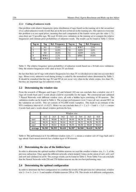
- Page 233: 218 Mannes Poel, Egwin Boschman and
- Page 237 and 238: 222 Mannes Poel, Egwin Boschman and
- Page 239 and 240: 224 Mannes Poel, Egwin Boschman and
- Page 241 and 242: 226 Marc Ponsen et al. Therefore, t
- Page 243 and 244: 228 Marc Ponsen et al. is playing t
- Page 245 and 246: 230 Marc Ponsen et al. (a) (b) (c)
- Page 247 and 248: 232 Marc Ponsen et al. on the switc
- Page 249 and 250: 234 Steven Roebert, Tijn Schmits an
- Page 251 and 252: 236 Steven Roebert, Tijn Schmits an
- Page 253 and 254: 238 Steven Roebert, Tijn Schmits an
- Page 255 and 256: 240 Steven Roebert, Tijn Schmits an
- Page 257 and 258: 242 Maarten van Someren, Martin Poo
- Page 259 and 260: 244 Maarten van Someren, Martin Poo
- Page 261 and 262: 246 Maarten van Someren, Martin Poo
- Page 263 and 264: 248 Maarten van Someren, Martin Poo
- Page 265 and 266: 250 Eelke Spaak and Pim F.G. Hasela
- Page 267 and 268: 252 Eelke Spaak and Pim F.G. Hasela
- Page 269 and 270: 254 Eelke Spaak and Pim F.G. Hasela
- Page 271 and 272: 256 Eelke Spaak and Pim F.G. Hasela
- Page 273 and 274: 258 Ivo Swartjes and Mariët Theune
- Page 275 and 276: 260 Ivo Swartjes and Mariët Theune
- Page 277 and 278: 262 Ivo Swartjes and Mariët Theune
- Page 279 and 280: 264 Ivo Swartjes and Mariët Theune
- Page 281 and 282: 266 Gerben K.D. de Vries, Véroniqu
- Page 283 and 284: 268 Gerben K.D. de Vries, Véroniqu
- Page 285 and 286:
270 Gerben K.D. de Vries, Véroniqu
- Page 287 and 288:
272 Gerben K.D. de Vries, Véroniqu
- Page 289 and 290:
274 Arlette van Wissen, Jurriaan va
- Page 291 and 292:
276 Arlette van Wissen, Jurriaan va
- Page 293 and 294:
278 Arlette van Wissen, Jurriaan va
- Page 295 and 296:
280 Arlette van Wissen, Jurriaan va
- Page 298 and 299:
An Architecture for Peer-to-peer Re
- Page 300 and 301:
Enhancing the Performance of Maximu
- Page 302 and 303:
Modeling the Dynamics of Mood and D
- Page 304 and 305:
A Tractable Hybrid DDN-POMDP approa
- Page 306 and 307:
An Algorithm for Semi-Stable Semant
- Page 308 and 309:
Towards an Argument Game for Stable
- Page 310 and 311:
Temporal Extrapolation within a Sta
- Page 312 and 313:
Approximating Pareto Fronts by Maxi
- Page 314 and 315:
A Probabilistic Model for Generatin
- Page 316 and 317:
Self-organizing Mobile Surveillance
- Page 318 and 319:
Engineering Large-scale Distributed
- Page 320 and 321:
A Cognitive Model for the Generatio
- Page 322 and 323:
Opponent Modelling in Automated Mul
- Page 324 and 325:
Exploring Heuristic Action Selectio
- Page 326 and 327:
Individualism and Collectivism in T
- Page 328 and 329:
Agents Preferences in Decentralized
- Page 330 and 331:
Agent-based Patient Admission Sched
- Page 332 and 333:
An Empirical Study of Instance-base
- Page 334 and 335:
The Importance of Link Evidence in
- Page 336 and 337:
Evolutionary Dynamics for Designing
- Page 338 and 339:
Combining Expert Advice Efficiently
- Page 340 and 341:
Paying Attention to Symmetry Gert K
- Page 342 and 343:
Of Mechanism Design and Multiagent
- Page 344 and 345:
Metrics for Mining Multisets 1 Walt
- Page 346 and 347:
A Hybrid Approach to Sign Language
- Page 348 and 349:
Improved Situation Awareness for Pu
- Page 350 and 351:
Authorship Attribution and Verifica
- Page 352 and 353:
Agent Performance in Vehicle Routin
- Page 354 and 355:
Design and Validation of HABTA: Hum
- Page 356 and 357:
Improving People Search Using Query
- Page 358 and 359:
The tOWL Temporal Web Ontology Lang
- Page 360 and 361:
A Priced Options Mechanism to Solve
- Page 362 and 363:
Autonomous Scheduling with Unbounde
- Page 364 and 365:
1 Introduction Don’t Give Yoursel
- Page 366 and 367:
Audiovisual Laughter Detection Base
- Page 368 and 369:
P 3 C: A New Algorithm for the Simp
- Page 370 and 371:
OperA and Brahms: a symphony? 1 Int
- Page 372 and 373:
Monitoring and Reputation Mechanism
- Page 374 and 375:
Subjective Machine Classifiers Denn
- Page 376 and 377:
Single-Player Monte-Carlo Tree Sear
- Page 378 and 379:
Mental State Abduction of BDI-Based
- Page 380 and 381:
Decentralized Performance-aware Rec
- Page 382 and 383:
Combined Support Vector Machines an
- Page 384 and 385:
Reconfiguration Management of Crisi
- Page 386 and 387:
Decentralized Online Scheduling of
- Page 388 and 389:
Polynomial Distinguishability of Ti
- Page 390 and 391:
Decentralized Learning in Markov Ga
- Page 392 and 393:
Organized Anonymous Agents ∗ Mart
- Page 394 and 395:
Topic Detection by Clustering Keywo
- Page 396 and 397:
Modeling Agent Adaptation in Games
- Page 398 and 399:
Monte-Carlo Tree Search Solver 1 Ma
- Page 400:
Demonstrations BNAIC 2008
- Page 403 and 404:
388 Joost Batenburg and Walter Kost
- Page 405 and 406:
390 Guillaume Chaslot, Sander Bakke
- Page 407 and 408:
392 Dennis Hofs, Mariët Theune and
- Page 409 and 410:
394 François L.A. Knoppel, Almer S
- Page 411 and 412:
396 Dirkjan Krijnders and Tjeerd An
- Page 413 and 414:
398 Joris Maervoet, Patrick De Caus
- Page 415 and 416:
400 Thomas Mensink and Jakob Verbee
- Page 417 and 418:
402 Daniel Okouya and Virginia Dign
- Page 419 and 420:
404 Roeland Ordelman et al. After t
- Page 421 and 422:
406 Dennis Reidsma and Anton Nijhol
- Page 423 and 424:
408 Michel F. Valstar, Simon Colton
- Page 425 and 426:
410 Tim Verwaart and John Wolters 2
- Page 427 and 428:
K Kaisers, Michael . . . . . . . .


