pdf 349K - Stanford Exploration Project - Stanford University

Stanford Exploration Project, Report 108, April 29, 2001, pages 1–?? 

A least-squares approach for estimating integrated velocity 

models from multiple data types 

Morgan Brown and Robert G. Clapp 1 

ABSTRACT 

Many exploration and drilling applications would benefit from a robust method of integrating 

vertical seismic profile (VSP) and seismic data to estimate interval velocity. In 

practice, both VSP and seismic data contain random and correlated errors, and integration 

methods which fail to account for both types of error encounter problems. We present a 

nonlinear, tomography-like least-squares algorithm for simultaneously estimating an interval 

velocity from VSP and seismic data. On each nonlinear iteration of our method, we 

estimate the optimal shift between the VSP and seismic data and subtract the shift from 

the seismic data. In tests, our algorithm is able to resolve an additive seismic depth error, 

caused by a positive velocity perturbation, even when random errors are added to both 

seismic and VSP data. 

INTRODUCTION 

Although the interval velocities obtained from surface seismic data normally contain errors 

(caused by poor processing, anisotropy, and finite aperture effects, among other factors), 

prospects are often drilled using only depth-converted seismic data. Unsurprisingly, depth 

converted seismic data often poorly predicts the true depth of important horizons. This “mistie” 

is more than a mere inconvenience; inadvertently drilling into salt (Payne, 1994) or into an 

overpressured layer (Kulkarni et al., 1999) can result in expensive work interruptions or dangerous 

drilling conditions. For depth conversion, vertical seismic profile (VSP) data generally 

produces better estimates of interval velocity than does surface seismic data. For this reason, 

VSP data has been used to “calibrate” seismic velocities to improve depth conversion, before, 

during, and after drilling. 

Methods to independently estimate interval velocity from VSP and surface seismic data 

exist and are more or less mature. Surprisingly, there exists no robust, “industry-standard” 

method for jointly integrating these two data types to estimate a common velocity model. The 

main challenge in developing such a method lies in measuring and accounting for the errors 

between each data type. Data errors may be either random or correlated, or most commonly, 

both. A viable integration scheme must account for both types of error. 

Some calibration algorithms (Ensign et al., 2000) directly compute the depth misfit be- 

1 email: morgan@sep.stanford.edu,bob@sep.stanford.edu 

1

2 Brown and Clapp SEP–108 

tween depth-converted seismic and VSP data (or sonic log picks) and use it to compute a 

correction velocity. The reliability of such algorithms is hampered by the assumption that the 

VSP data is error-free, when in fact, these data have random (hopefully) first-break-picking 

errors and also possibly exhibit correlated errors resulting from correction of deviated well 

VSP data to vertical (Noponen, 1995). 

Various authors have employed least-squares optimization algorithms to solve a related 

problem: the estimation of an optimal time shift to tie crossing 2-D seismic lines at the intersections 

(Bishop and Nunns, 1994; Harper, 1991). While these algorithms correctly assume 

that all data has errors, they assume that these errors are uncorrelated, or in other words, that 

the data are realizations of the same random variable. We expect seismic time/depth pairs to 

differ from VSP time/depth pairs by a low frequency shift, and that both data have random 

errors. Figure 1 illustrates this relationship as shifted probability distribution functions. A 

common view in practice, and one espoused by geostatistics, is that the inherent inaccuracy, 

or “softness” of seismic data causes the observed misfit between seismic and wellbore data 

(Mao, 1999). No attempt is made to estimate the joint data correlation, and the net effect is a 

faulty assumption that the seismic data is less accurate than it really is. 

In this paper, we present a nonlinear least-squares algorithm using VSP and surface seismic 

data for the simultaneous estimation of interval velocity and an additive seimic correction 

velocity. We test the algorithm on a real VSP dataset. To simulate seismic data, we perturb 

the VSP data with depth errors derived from a positive velocity anomaly. The tests show that 

our algorithm correctly handles the errors in VSP data and leads to an unbiased residual. We 

also add random errors to both the VSP and seismic data and show that by assuming that the 

data are correlated, we can improve the final result. 

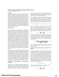
Figure 1: We assume that seismic 

time/depth pairs differ from VSP 

time/depth pairs by a shift (due to 

poor processing, anisotropy, finite 

aperture effects, etc.), and that both 

are random variables. The respective 

probability distribution functions 

(pdf’s) are displayed as bell shaped 

curves. If the seismic data are considered 

soft, and no effort is made to estimate 

correlated errors (shift in pdf), 

then a common, incorrect tendency is 

to assume that the seismic data are 

much less accurate than they are in reality. 

morgan1-soft [NR] 

VSP Seismic 

T/D pair T/D pair 

Observed Δ z 

Assume 

correlated 

error 

Assume 

seismic is 

soft data

SEP–108 Integrated velocity estimation 3 

LEAST SQUARES FORMULATION 

The fundamental data unit of this paper is the “time/depth pair”, which is quite simply the 

traveltime of seismic waves to a specified depth, along an assumed vertical raypath. We denote 

time depth pairs by (τp,ζp), indexed by p, the “pair” index. The output velocity function is 

linear within layers. We denote layer boundaries, which are independent of the time/depth 

pairs, by tl, indexed by l, the “layer” index. We begin by deriving the 1-D data residual – the 

depth error between the depth component of a time/depth pair (ζp) and its time component 

(τp) after vertical stretch with the (unknown) interval velocity: 

ep = ζp − 

� τp 

0 

v(t)dt. (1) 

For implementation purposes, we break the integral into the sum of integrals between neighboring 

time/depth pairs (t = [τp,τp+1]): 

ep = ζp − 

p� 

q=1 

� τq 

τq−1 

We assume that the interval velocity in layer l is linear, 

v(t)dt. (2) 

v(t) = v0,l + klt; {t = [tl,tl+1]}, (3) 

so the integral in equation (2) has a closed form. To obtain a correspondence between time/depth 

pairs and layer boundaries, note that, given a time/depth pair, we can always determine in 

which layer it resides. In other words, we can unambiguously write l as a function of p, l[p]. 

Now we can evaluate the integrals of equation (2): 

ep = ζp − 

p� 

q=1 

v0,l[q](τq+1 − τq) + kl[q] 

2 (τ 2 q+1 − τ 2 q ). (4) 

Equation (4) defines the misfit for a single time/depth pair, as a function of the model parameters 

2 . Now pack the individual misfits from equation (4) into a residual vector, rd: 

� 

v0 

rd = ζ − A 

k 

� 

≈ 0 (5) 

The elements of vector ζ are the time/depth pair depth values, A is the summation operator 

suggested by equation (4). and [v0 k] T is the unknown vector of intercept and slope parameters. 

The primary goal of least squares optimization is to minimize the mean squared error of 

the data residual, hence the familiar fitting goal (≈) notation. 

2 Equation (4) implictly assumes that layer boundaries do not occur between time/depth pairs. The code 

does not make this assumptions: layer boundaries can occur anywhere in time, and are completely independent 

of the time/depth pairs. When a layer boundary lies between time/depth pairs p and p + 1, the integral 

has two parts: depth contribution from above and below the layer boundary.


1-D Model Regularization: Discontinuity Penalty 

In many applications, the interval velocity must be smooth across layer boundaries. To accomplish 

this, we incorporate a penalty on the change in velocity across the layer boundary, 

and effectively exchange quality in data fit for a continuous result. However, as mentioned 

by Lizarralde and Swift (1999), an accumulation of large residual errors would result if we 

forced continuity in the velocity function across layer boundaries with large velocity contrast. 

Therefore we “turn off” the discontinuity penalty at certain layers via a user-defined “hard 

rock” weight. 

Let us write the weighted discontinuity penalty at the boundary between layers l and l +1: 

w h l 

� 

v0,l + kltl − � �� 

v0,l+1 + kl+1tl 

wh l is the hard rock weight. We suggest that the wh l be treated as a binary quantity: either 1 for 

soft rock boundaries or 0 for hard rock boundaries. As before, we write the misfits of equation 

(6) in fitting goal notation and combine with equation (5): 

� A 

ɛC 

�� v0 

k 

C is simply the linear operator suggested by equation (6): a matrix with coefficients of ±1 

and ±tl, with rows weighted by the wh l . Application of C is tantamount to applying a scaled, 

discrete first derivative operator to the model parameters in time. The scalar ɛ controls the 

trade off between model continuity and data fitting. Lizarralde and Swift (1999) give a detailed 

strategy for choosing ɛ. 

� 

≈ 

Estimating and Handling Random Data Errors 

In this paper, we assume zero-offset VSP (ZVSP) data. We derive a simple measure of ZVSP 

data uncertainty below. The uncertainty in surface seismic data depends on velocity and raypath 

effects in a more complex manner, although Clapp (2001) has made encouraging progress 

in bounding the uncertainty. Somewhat counter to intuition, we adopt the convention that traveltime 

is the independent variable in a time/depth pair, i.e., z = f (t). Bad first break picks and 

ray bending introduce errors into the traveltimes of ZVSP data, but depth in the borehole to the 

receiver is well known. To obtain an equivalent depth error, we need only scale the traveltime 

error in ZVSP data by the average overburden velocity. By definition, the traveltime t (along 

a straight ray) is related to depth z in the following way: 

� ζ 

0 

� 

(6) 

(7) 

z = tvavg, (8) 

where vavg is the average overburden velocity. If the traveltime is perturbed with error �t it 

follows that the corresponding depth error, �z is simply the traveltime error scaled by vavg: 

�z = �tvavg. (9)


If the data errors are independent and follow a Gaussian distribution, least squares theory prescribes 

(Strang, 1986) that the data residual of equation (5) be weighted by the inverse variance 

of the data. Assuming that we have translated a priori data uncertainty into an estimate of data 

variance, we can define a diagonal matrix W where the diagonal elements wii = σ −1 

i : the 

inverse of the variance of the i th datum. This diagonal operator is applied to the data residual 

of equation (7): 

� WA 

ɛC 

�� v0 

k 

� 

≈ 

Estimating and Handling Correlated Data Errors 

� Wζ 

0 

We assume that the measured VSP depths, ζ vsp, consist of the “true” depth, ˜ζ , plus a random 

error vector, evsp: 

ζ vsp = ˜ζ + evsp 

Furthermore, we assume that the measured seismic depths, ζ seis, are the sum of the true depth, 

a random error vector, eseis, and a smooth perturbation, �ζ : 

� 

(10) 

(11) 

ζ seis = ˜ζ + eseis + �ζ (12) 

When the data residuals are correlated, the optimal choice for W in equation (10) becomes 

the square root of the inverse data covariance matrix. Guitton (2000) noted that after applying 

a hyperbolic Radon transform (HRT) to a CMP gather, coherent noise events, which are not 

modeled by the HRT, appear in the data residual. He iteratively estimated a prediction error 

filter from the data residual and used it as the (normalized) square root of the inverse data 

covariance. 

If we subtract �ζ from ζ seis, then the error is random, as desired. Unfortunately, �ζ 

is unknown. We iteratively estimate �ζ , and the velocity pertubation which is assumed to 

produce �ζ , �v, using the following tomography-like iteration: 

�ζ = 0 

iterate { 

} 

Solve equation (10) for v = [v0 k] T : 

Solve equation (10) for �v: 

�ζ = A�v 

� WA 

ɛC 

� WA 

ɛC 

� � 

W(ζ + �ζ ) 

v ≈ 

0 

� � 

W(Av − ζ ) 

�v ≈ 

0 

The first stage of the iteration solves equation (10) for an interval velocity function, using 

the VSP data, and the corrected seismic data. In the second stage of the iteration, we estimate 

� 

�


a correction velocity function from the residual, which is similar to Guitton’s approach. By 

forcing the correction velocity to obey equation (10), we force it to be “reasonable”, and hence, 

we ensure that the estimated correction depth results from this reasonable velocity. One future 

feature that we envision is the ability to force the correction velocity to be zero in one or more 

layers. For example, if we had strong evidence to believe that most of the seismic/VSP mistie 

was caused by anisotropy in one prominent shale layer, we might only want nonzero correction 

velocity in this layer. 

By forcing the correction velocity to be reasonable (continuous, for example), our estimated 

depth correction may not fully decorrelate the residual in the first step of the iteration. 

For this reason, we must do more than one iteration. We find that for this example, the correction 

velocity changes very little after 15 nonlinear iterations, and that 5 nonlinear iterations 

gives a decent result. 

We admit that our nonlinear iteration may be risky. We have solved a very simple analog 

to the classic reflection tomography problem, where traveltimes depend both on reflector 

position and on velocity. Our approach was to completely decouple optimization of velocity 

from correction depth. Modern tomography approaches attempt to simultaneously optimize 

reflector position and velocity, and we should attempt to improve our method similarly. 

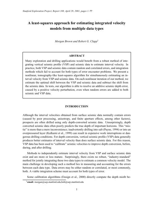
REAL DATA RESULTS 

Figure 2 illustrates the experiment. A VSP, donated by Schlumberger, is overlain by first 

break picks, obtained by picking from the first trace and crosscorrelating. Layer boundaries 

are shown as horizontal lines. Most layers contain more than three time/depth pairs. In some 

regions, the waveform is quite crisp, and the picks predictably appear accurate. In other regions, 

notably after 1.8 seconds, the wavelet coherency and amplitude are degraded, and the 

picks appear “jittery”. Nonetheless, we assume a variance of 0.006 seconds in the picked VSP 

traveltimes, and compute the equivalent depth uncertainty from equation (9). The inverse of 

the depth uncertainty is directly input as the residual weight to equation (10). Figures 3-6 illustrate 

the scheme we proposed earlier for simultaneously inverting VSP and surface seismic 

time/depth pairs for interval velocity. 

Figure 3 is the “proof of concept”. We simply add a positive correlated depth error, corresponding 

to “anisotropy” in layers 2-4, to the VSP time/depth pairs to simulate surface seismic 

data. The topmost panel contains the known (solid line) and the estimated (+) velocity perturbations. 

Our algorithm has reconstructed the known velocity perturbation quite well. The 

second panel from top shows the depth error produced by backprojecting the known (solid 

line) and estimated (+) velocity perturbations. The center panel contains the VSP (v) and 

seismic (s) time/depth pairs. The solid line shows the modeled depth, or the backprojected 

final estimated velocity. The second panel from bottom shows the estimated velocity function. 

Notice that we have declared 4 of the 26 layer boundaries as “hard rock” boundaries, 

per equation (6), in order to suppress large residual errors from occuring across the obviously 

high-velocity-contrast layer boundaries. Inspecting the bottom panel, we see that the residual 

appears uncorrelated.


Figure 2: Left: Schlumberger VSP, with first break picks (-) and layer boundaries (horizontal 

lines). Right: Residual weight associated with first break picks. morgan1-showvsp [ER]


Figure 4 illustrates that failure to account for correlated errors leads to an undesirable 

result. In this case, we add the same correlated depth error as in Figure 3 to simulate seismic 

data. Additionally, we add to the seismic data random errors with a standard deviation of 

0.024 seconds, four times the assumed standard deviation of the VSP data. Finally, we add 

random errors with the same standard deviation (0.024 sec) to the VSP data, in the interval 

[1.25 1.46] seconds, to simulate a region of poor geophone coupling. We do not perform the 

correlated data error iteration outlined above, but instead simply solve equation (10). The 

most important panel to view is the residual panel; without explictly modeling the correlated 

errors, least squares optimization simply “splits the difference” between VSP and seismic 

error, causing bias in both. The v’s correspond to VSP errors, the s’s to seismic errors. 

Figure 5 shows the application of our algorithm to the data of Figure 4. Instantly, we see 

that the estimated velocity perturbation and correlated depth error match the known curves 

reasonably well. The estimated perturbations don’t match as well as in Figure 3 because of 

the random errors. The residual is random, though it appears to be poorly scaled in the region 

where we added random noise to the VSP. In fact, we have used the same residual weight as 

shown in Figure 2. If we know that we have bad data, we should reduce the residual weight 

accordingly. Additionally, we see that the final velocity function doesn’t look as much like the 

“known” result of Figure 3, which had no additive random noise. 

Figure 6 is the same as Figure 5, save for a change to the residual weight. We reduce the 

residual weight in the [1.25 1.46] sec. interval by a factor of 4. We notice first that the residual 

is both random and well-balanced. Also note that the estimated final velocity function much 

more resembles that of Figure 3, which is good. The modeled data, in the center panel, is 

nearly halfway in between the VSP and seismic data in the region of poor VSP data quality, 

which makes sense, since we have reduced the residual weight. 

The last example underscores an important philosophical point, which we emphasized in 

the introduction and in Figure 1. All too often, when different data types fail to match, the 

differences are chalked up to the inaccuracy of the “soft data”. In effect, by failing to account 

for correlated error, they assume that the soft data has a much larger variance than it really 

does. Our algorithm effectively adjusts the mean of the seismic pdf to match the mean of the 

VSP pdf. 

In this example, we see that after removing the correlated error, the soft data (seismic) has 

in fact improved the final result, because the velocity more closely resembles that in Figure 3. 

Don’t throw away the data! Use physics to model correlated errors and remove them from the 

data. It may not be as soft as you think.


Figure 3: Proof-of-concept plot. Positive depth perturbation (but no random errors) added to 

seismic time/depth pairs. morgan1-misfit1 [ER]


DISCUSSION 

We have developed an algorithm to simultaneously invert VSP and seismic time/depth pairs 

for interval velocity, in cases when the VSP data contains random errors and the seismic data 

contains both random and correlated errors. Our algorithm utilizes a nonlinear iteration, where 

we decouple estimation of the correlated depth error and velocity. This decoupling is in general 

a risky strategy, and although our results are reasonable, we should explore alternatives. 

Extension of the algorithm to 2-D and 3-D is the next important issue. Modern wells are 

deviated, and many operators expend considerable resources to acquire “source-over-receiver” 

VSP data, in order to ensure vertical raypaths (Noponen, 1995). In this scenario, the subsurface 

is sparsely sampled by the VSP at any given spatial location. The sparsity is the main reason 

why we parameterize the interval velocity as a piecewise linear function. Layer-constant 

velocities are even less parameter-intensive. 

We assumed that the errors in VSP data are random. This is likely untrue in practice, but 

more research is needed. In the future, we may attempt to estimate correlated error in all data 

sources with the nonlinear iteration. We would also like to incorporate additional data types 

into our algorithm, such as well logs. 

ACKNOWLEDGEMENTS 

The first author acknowledges the following people at Landmark Graphics for valuble discussions 

on this topic during his 2000 internship: Phil Ensign, Andreas Rüger, Lydia Deng, and 

Bill Harlan. We also acknowledge Antoine Guitton for editorial assistance. 

REFERENCES 

Bishop, T. N., and Nunns, A. G., 1994, Correcting amplitude, time, and phase mis-ties in 

seismic data: Geophysics, 59, no. 6, 946–953. 

Clapp, R. G., 2001, Multiple realizations: Model variance and data uncertainty: SEP–108, 

147–158. 

Ensign, P., Harth, P., and Davis, B., 2000, Rapidly and automatically tying time to depth using 

sequential volume calibration: 70th Annual Internat. Mtg., Soc. Expl. Geophys., Expanded 

Abstracts, Session: INT 6.4. 

Guitton, A., 2000, Coherent noise attenuation using Inverse Problems and Prediction Error 

Filters: SEP–105, 27–48. 

Harper, M. D., 1991, Seismic mis-tie resolution technique: Geophysics, 56, no. 11, 1825– 

1830.


Figure 4: Random errors added to VSP and seismic data of Figure 3. Correlated errors not 

handled. Residual is biased. morgan1-misfit2 [ER]


Figure 5: Application of our algorithm to data of Figure 4. Residual is random, but poorly 

scaled in region where VSP random errors are larger. morgan1-misfit3 [ER]


Figure 6: Same data as in Figure 5, residual weight reduced in region where VSP random 

errors are larger. Here, the “soft” seismic data has actually improved the velocity estimate, as 

it more closely resembles Figure 3. morgan1-misfit4 [ER]


Kulkarni, R., Meyer, J., and Sixta, D., 1999, Are pore pressure related drilling problems predictable? 

The value of using seismic before and while drilling: 69th Annual Internat. Mtg., 

Soc. Expl. Geophys., Expanded Abstracts, 172–175. 

Lizarralde, D., and Swift, S., 1999, Smooth inversion of VSP traveltime data: Geophysics, 64, 

no. 3, 659–661. 

Mao, S., 1999, Multiple layer surface mapping with seismic data and well data: Ph.D. thesis, 

Stanford University. 

Noponen, I. T., 1995, Velocity computation from checkshot surveys in deviated wells (short 

note): Geophysics, 60, no. 6, 1930–1932. 

Payne, M. A., 1994, Looking ahead with vertical seismic profiles: Geophysics, 59, no. 08, 

1182–1191. 

Strang, G., 1986, Introduction to applied mathematics: Wellesley-Cambridge Press.

pdf 349K - Stanford Exploration Project - Stanford University

Create successful ePaper yourself

Delete template?

Save as template?