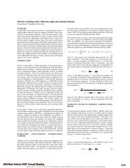
8 Brown and Clapp SEP–108 Figure 4 illustrates that failure to account for correlated errors leads to an undesirable result. In this case, we add the same correlated depth error as in Figure 3 to simulate seismic data. Additionally, we add to the seismic data random errors with a standard deviation of 0.024 seconds, four times the assumed standard deviation of the VSP data. Finally, we add random errors with the same standard deviation (0.024 sec) to the VSP data, in the interval [1.25 1.46] seconds, to simulate a region of poor geophone coupling. We do not perform the correlated data error iteration outlined above, but instead simply solve equation (10). The most important panel to view is the residual panel; without explictly modeling the correlated errors, least squares optimization simply “splits the difference” between VSP and seismic error, causing bias in both. The v’s correspond to VSP errors, the s’s to seismic errors. Figure 5 shows the application of our algorithm to the data of Figure 4. Instantly, we see that the estimated velocity perturbation and correlated depth error match the known curves reasonably well. The estimated perturbations don’t match as well as in Figure 3 because of the random errors. The residual is random, though it appears to be poorly scaled in the region where we added random noise to the VSP. In fact, we have used the same residual weight as shown in Figure 2. If we know that we have bad data, we should reduce the residual weight accordingly. Additionally, we see that the final velocity function doesn’t look as much like the “known” result of Figure 3, which had no additive random noise. Figure 6 is the same as Figure 5, save for a change to the residual weight. We reduce the residual weight in the [1.25 1.46] sec. interval by a factor of 4. We notice first that the residual is both random and well-balanced. Also note that the estimated final velocity function much more resembles that of Figure 3, which is good. The modeled data, in the center panel, is nearly halfway in between the VSP and seismic data in the region of poor VSP data quality, which makes sense, since we have reduced the residual weight. The last example underscores an important philosophical point, which we emphasized in the introduction and in Figure 1. All too often, when different data types fail to match, the differences are chalked up to the inaccuracy of the “soft data”. In effect, by failing to account for correlated error, they assume that the soft data has a much larger variance than it really does. Our algorithm effectively adjusts the mean of the seismic <strong>pdf</strong> to match the mean of the VSP <strong>pdf</strong>. In this example, we see that after removing the correlated error, the soft data (seismic) has in fact improved the final result, because the velocity more closely resembles that in Figure 3. Don’t throw away the data! Use physics to model correlated errors and remove them from the data. It may not be as soft as you think.
SEP–108 Integrated velocity estimation 9 Figure 3: Proof-of-concept plot. Positive depth perturbation (but no random errors) added to seismic time/depth pairs. morgan1-misfit1 [ER]