Evaluación y simulación precoces del crecimiento de ... - FCF UNSE

Quebracho N° 7 (31-42)
EVALUACIÓN Y SIMULACIÓN PRECOCES DEL CRECIMIENTO
DE RODALES DE Pinus taeda L. CON MATRICES DE TRANSICIÓN
Precocious growth evaluation and simulation with
transition matrixes for Pinus taeda stands
C. R. Sanquetta 1 , J. E. Arce 1 , F. dos Santos Gomes 1 , E. Coutinho da Cruz 2
RESUMEN
Es evaluado y simulado el crecimiento de
rodales jóvenes, coetáneos, monoespecíficos y
homogéneos de Pinus taeda L. utilizando la
técnica de simulación Matrices de Transición.
Los datos utilizados provienen de mediciones
realizadas en árboles individuales en 1993 y 1996
(6 o y 9 o años) en un ensayo de espacia-mientos
de Pinus taeda L., instalado en el municipio de
Jaguariaíva - PR, en la Fazenda Lageado,
propiedad de la empresa “Pisa Florestal”. La
construcción de las matrices de transición a partir
de observaciones diamétricas obtenidas de
rodales de Pinus taeda en dos oportunidades,
separadas entre sí por un intervalo de tiempo
dado, es factible y permite obtener simulaciones
coherentes para un período de tiempo igual al
considerado. La simulación para intervalos de
tiempo mayores que el período utilizado en la
construcción de las matrices de transición no es
recomendable, por tratarse de rodales jóvenes y
no estar disponible, por lo tanto, información del
ciclo completo de la dinámica del bosque.
Palabras clave : crecimiento, simulación, matrices
de transición, Pinus taeda, distribuciones
diamétricas.
Recibido en marzo de 1997; aceptado en febrero de 1998
1 Universidad Federal del Paraná (UFPR), Rua Bom Jesus 650 – Juveve 80.035-010 Curitiba - PR, Brasil.
2 Universidad Federal del Amazonas. Brasil.
ABSTRACT
The growth of young, even-aged,
monospecific and homogeneous stands of Pinus
Taeda L. are evaluated and simulated with the
Transition Matrix simulation technique. The used
data was obtained from measurements over
individual trees in 1993 and 1996 (6 th and 9 th years)
in an spacing test of Pinus taeda L. at farm
Fazenda Lageado in Jaguariaiva - PR, from the
Pisa Florestal company. The transition matrixes
construction from two diameter observations
separated by a time interval are feasible and
conduce to coherent simulations for a similar time
interval that the used for the transition matrixes
construction. Simulations for longer time intervals
that the used for the transition matrixes
construction are not recommended because the
sampled stands are young and it is not
disposable information about the complete
dynamic cycle of the forest.
Key words: growth, simulation, transition
matrices, Pinus taeda, diameter distributions.

32 Revista de Ciencias Forestales – Quebracho N° 7 – Junio 1999
1. INTRODUCCIÓN
Un manejo forestal efectivo implica la aplicación de un sistema de tratamientos para el
control de la masa forestal, de tal manera que el incremento en el valor económico y/o social del
bosque sea más rápido que los intereses acumulados de los costos de los tratamientos (Alder,
1980). Al mismo tiempo, todas las operaciones de exploración disminuirán la masa futura en
mayor o menor grado. Una tasa de exploración muy alta traerá como consecuencia final la
liquidación del recurso forestal; una tasa muy baja puede privar a la comunidad de recursos
inmediatos y reducir el potencial de crecimiento futuro del bosque (Alder, 1980). Un modelo de
predicción del rendimiento debe ser capaz de evaluar todos los factores relacionados con el
manejo forestal, si es que se quiere utilizarlo plenamente en la toma de decisiones de la empresa
forestal (Clutter, et al., 1983).
El manejo silvícola dentro de un rodal puede ser realizado árbol por árbol, o por
agrupamientos, pero el mayor interés de la ingeniería forestal se centra en el efecto de los
tratamientos sobre el volumen, el valor o la estructura, de la totalidad del rodal (Daniel, et al.,
1982).
El crecimiento de los rodales puros coetáneos se ve afectado por el estado de desarrollo del
bosque, la calidad de sitio, la especie, la densidad - expresada en área basal y en número de
árboles por unidad de superficie -, los tratamientos silviculturales, y las unidades en las que es
expresado el crecimiento. La densidad del rodal es el segundo factor en importancia, después de
la calidad de sitio, para la determinación de la productividad de un sitio forestal (Daniel, et al.,
1982), para una determinada calidad del material genético utilizado. La densidad del rodal es el
principal factor de producción que el silvicultor puede manejar durante el desarrollo del bosque.
La estimación del crecimiento es una etapa esencial en la ordenación forestal. Cualquier
planificación implica la predicción del crecimiento (Spurr, 1952). Una correcta estimación de la
productividad forestal de un sitio, expresada en m 3 /ha, proporciona una herramienta útil y
necesaria de planeamiento y administración de la empresa forestal.
Solamente podrán ser tomadas decisiones racionales a respecto de la intensidad y épocas de
raleos y de la cosecha final, si la respuesta de los bosques a estas operaciones puede ser
cuantificada. Los estudios de crecimiento y rendimiento son los medios utilizados para alcanzar
este fin (Alder, 1980).
El estudio y la modelización del crecimiento y de la producción forestal es de fundamental
importancia para la implementación de técnicas de manejo y planeamiento forestal. El proceso
de decisión en el manejo forestal requiere del conocimiento de todas las variables envueltas en el
proceso productivo, como también de la evolución de la producción del rodal. Los modelos de
simulación son actualmente imprescindibles para el correcto desarrollo de técnicas que buscan
obtener la máxima productividad del bosque y la máxima rentabilidad del emprendimiento.
Alder (1980), Clutter et al. (1983) y Davis y Johnson (1987) clasificaron a los modelos de
crecimiento y producción en tres tipos:
• Modelos globales de rodal, que permiten obtener una estimación general de la
producción por unidad de área;
• Modelos por clases diamétricas, que posibilitan la prognosis del número de árboles
por clase diamétrica. La altura, el volumen y otras características del rodal pueden
ser asociadas a cada una de esas clases; y,
• Modelos para árboles individuales, que consideran características de árboles
individuales para la prognosis del crecimiento y producción del rodal.
Los modelos por clase diamétrica utilizan normalmente funciones de densidad de
probabilidades para la obtención de las frecuencias de los árboles en cada clase diamétrica. Las
variables independientes más comunes para las prognosis son el número de árboles por hectárea,
la edad y la altura dominante del rodal.

Sanquetta et al.: Evaluación y simulación... 33
Según Sanquetta (1996), tres modelos no espaciales expresan el desarrollo del rodal por
medio de la descripción de la evolución de las distribuciones diamétricas o de otra variable en
clases, y son conocidos como funciones probabilísticas, matrices de transición y procesos de
difusión.
La matriz de transición es un proceso estocástico utilizado para estudiar fenómenos que
pasan a partir de un estado inicial por una secuencia de estados, donde la transición de un
determinado estado ocurre según una cierta probabilidad. Los puntos más importantes en el
montaje de una Cadena de Markov son la definición de estados del sistema y la construcción de
la matriz de transición probabilística (Hoyos, 1980). De acuerdo con Enright y Ogden (1979), el
único requisito para la utilización del modelo matricial es que la población pueda ser dividida en
estados o compartimentos, y que exista la probabilidad de movimiento de un estado para otro en
el tiempo.
De acuerdo con Sanquetta (1996), en las matrices de transición se utiliza el criterio de
separar árboles de una cierta clase diamétrica que avanzan para una, dos o más clases
consecutivas de aquellos que permanecen en la misma clase o mueren durante un intervalo de
tiempo dado. Esta dinámica de clases determina las probabilidades que constituyen los elementos
de la matriz de transición.
Muchos ejemplos de modelos con matrices de transición han sido utilizados para simular la
dinámica de poblaciones forestales. En la gran mayoría de los casos, la población es dividida en
clases diamétricas y la proyección de la frecuencia en estas clases se basa en el
comportamiento observado en un determinado período de tiempo.
La proyección del crecimiento diamétrico por medio de matrices de transición ya fue
estudiada por diversos investigadores. Entre ellos pueden ser citados: Bruner y Moser Jr. (1973)
en un rodal de frondosas mixtas en Wisconsin-EUA; Enright y Ogden (1979) en poblaciones de
Araucaria sp. del bosque tropical húmedo de Papua-Nueva Guinea y de Nothofagus fusca de
los bosques templadas de Nova Zelandia; Robert y Hruska (1986) en rodales de Pinus sp. en los
Estados Unidos; Buongiorno y Michie (1980) en rodales de Acer sacharum en Wisconsin y
Michigan en los EUA; y Mendoza y Setyarso (1986) como instrumento auxiliar en la
determinación del ciclo de corte en bosques de Indonesia.
Clutter y Bennett (op. cit. Bruner y Moser Jr., 1973) utilizaron, en rodales coetáneos, la
edad para computar cambios en las distribuciones diamétricas con el tiempo. La posibilidad de
describir la distribución diamétrica en diferentes edades a partir de la distribución probabilística
exponencial negativa fue sugerida por Leak (1965).
Lowell y Mitchell (1987) señalaron tres importantes limitaciones de la Cadena de Markov: 1)
es asumida una única calidad de sitio mientras que la dinámica de la población varía con el sitio;
2) cualquier árbol es tratado de la misma manera independientemente de las características
particulares del rodal; 3) la estructura del rodal es ignorada al ser considerada la misma dinámica
de la población, tanto para rodales coetáneos como disetáneos, puros o con una composición
variada de especies.
Un gran inconveniente de la utilización de la Cadena de Markov es la inflexibilidad del
modelo, ya que no permite hacer proyecciones para intervalos de tiempo que no sean múltiplos
del intervalo de medición. En este caso las estrategias de manejo quedan también condicionadas
a los años múltiplos del intervalo de medición (Harrison y Michie, 1985). Estos autores
desarrollaron un procedimiento para salvar esta restricción, por medio de la factorización de la
matriz de transición para períodos de un año. Para contornar la dificultad extrema de la
obtención de datos y de un número incontable de tablas, considerando una Cadena de Markov
para cada sitio y estructura, los mismos autores propusieron como alternativa el uso de
regresiones logísticas con variables de criterio (para modelar el crecimiento y la mortalidad) y,
además, otras variables auxiliares que describan el rodal en cuestión (diámetro medio, área
basal, altura dominante, stock de crecimiento, etc.).

34 Revista de Ciencias Forestales – Quebracho N° 7 – Junio 1999
El objetivo principal del presente estudio es evaluar y simular el crecimiento de rodales
jóvenes, coetáneos, monoespecíficos y homogéneos de Pinus taeda utilizando la técnica de
simulación Matrices de Transición.
2. MATERIALES
Los datos utilizados provienen de un ensayo de espaciamientos de Pinus taeda L., instalado
en el municipio de Jaguariaíva - PR, Fazenda Lageado, de propiedad de la empresa “Pisa
Florestal”, Proyecto J-2, cuadro 11. La plantación fue realizada entre los días 28 de octubre y 9
de noviembre de 1987, con plantines obtenidos a partir de semillas procedentes de Telêmaco
Borba - PR, de la empresa “Klabin Florestal”.
El área ocupada por el ensayo consta de seis bloques instalados de manera continua en un
total de 2,97 ha (incluyendo la bordura), con un área útil de 2,59 ha. El lugar de implantación del
ensayo poseía reforestación con Pinus taeda de 16 años de edad. A fines de 1986 fue realizada
una tala rasa en el proyecto. La limpieza del material resultante del aprovechamiento fue
realizada mediante una quema controlada, quedando el área, según los criterios de preparación
del terreno de la empresa, apta para la nueva plantación. La herramienta principal utilizada para
la plantación fue el azadón, el cual propició la abertura de hoyos con dimensiones medias de 20
cm de ancho por 15-20 cm de profundidad en formato de embudo. No fue realizado ningún tipo
de abonado. Conforme la necesidad y dentro de los patrones adoptados por la empresa, fueron
realizadas limpiezas en el ensayo.
El ensayo evalúa cinco espaciamientos, repetidos en seis bloques continuos. Cada parcela
posee doble bordura y son medidos solamente los árboles constantes de su área útil. Además, el
ensayo posee una doble bordura externa, buscando proporcionar el máximo de confiabilidad a las
inferencias. Los tratamientos del Diseño en Bloques Completos al Azar son los siguientes:
Área de la Parcela (m 2 Tratamiento
Espaciamiento
(m)
Árboles/ha
)
total útil
Plantas
útiles
1 2,5 x 1,2 3333 630 234 78
2 2,5 x 2,0 2000 630 210 42
3 2,5 x 2,8 1428 810 315 45
4 2,5 x 3,6 1111 990 378 42
5 2,5 x 4,4 909 1260 440 40
Las mediciones de DAP y altura total fueron realizadas anualmente, entre los años 1991 y
1996. Los datos utilizados en el presente trabajo corresponden a mediciones de árboles
individuales realizadas en 1993 y 1996 (6 o y 9 o años).
3. MÉTODOS
El primer análisis a ser realizado sobre los datos será testar la existencia de diferencias entre
los 5 tratamientos que justifiquen el estudio separado del crecimiento de cada uno de ellos. Las
diferencias serán analizadas por medio del test de comparación de medias (Tukey, α=0,05), para
los 5 tratamientos y los 6 períodos de observación (1991 a 1996).
La matriz de transición es un método de simulación que considera las frecuencias
diamétricas en el año de inicio de la simulación (Nt) como un vector, que multiplicado por una
matriz de probabilidades de transición entre clases diamétricas (Tp) permite obtener las
frecuencias diamétricas del año final (Nt+1). El ingreso es considerado también como un vector
(Rt), que es adicionado al producto vector-matriz descripto. La mortalidad puede ser considerada

Sanquetta et al.: Evaluación y simulación... 35
de dos maneras: como un vector de sustracción (Mt), o incluida en la matriz Tp en las últimas
línea y columna.
En álgebra de matrices, el proceso de simulación para 1 período (t → t+1), con la mortalidad
incluida en la matriz de transición, puede ser resumido como sigue:
N
{ t+ 1 = ( N Tp
{ t ' ⋅ ) + R
{ { t
( n+
1) × 1 t× ( n+
1) ( n+ 1) × ( n+
1) ( n+
1) × 1
y para simulaciones abarcando p períodos sin considerar el ingreso, que es el caso de los
bosques plantados de Pinus sp., el proceso de simulación queda:
N
{ t+ 1 = [ N
{ t ' ⋅ ( Tp)
123
]
( n+
1) × 1 1× ( n+
1) ( n+ 1) × ( n+
1)
donde (Tp) p es la matriz potencia de Tp, lo que en álgebra de matrices indica el producto de
la matriz Tp por si misma p veces (Tp 3 = Tp × Tp × Tp). Para que el producto sea factible, la
matriz Tp debe ser cuadrada (N o de líneas = N o de columnas).
La matriz de transición (Tp) esencialmente es una matriz de probabilidades, cuyos elementos
están descriptos a seguir:
⎡pf1
pa1 pb1 pc1 L L L L L pm1
⎤
⎢
⎥
⎢
pf2 pa2 pb2 pc2 L L L L pm2
⎥
⎢
pf pa pb pc pm ⎥
3 3 3 3 L L L 3
⎢
⎥
⎢
M M M ⎥
⎢
pfi pai pbi pci pm ⎥
i
Tp = ⎢
⎥
⎢
M M M ⎥
⎢
M M M ⎥
⎢
⎥
⎢
pfn−1 pan−1 pmn−1
⎥
⎢
⎥
⎢
pfn pmn
⎥
⎣⎢
1 ⎦⎥
donde:
pfi = probabilidad de que los árboles de la clase i permanezcan en la clase i durante (t → t+1);
pai = probabilidad de que los árboles de la clase i avancen para la clase i+1 (t → t+1);
pbi = probabilidad de que los árboles de la clase i avancen para la clase i+2 (t → t+1);
pci = probabilidad de que los árboles de la clase i avancen para la clase i+3 (t → t+1);
pmi = probabilidad de que los árboles de la clase i se mueran durante el período (t → t+1);
i = número de la clase diamétrica, variando desde 1 hasta n (última clase).
Los vectores de frecuencias observadas (Nt) y de ingresos (Rt) representan unidades físicas
(árboles) por clases diamétricas presentes en el inicio de la simulación e ingresadas durante el
período t+1, respectivamente. Por tratarse de bosques plantados el ingreso puede ser
despreciado y el vector Rt considerado como un vector nulo. El vector Nt es representado como
sigue:
N ' N N N L N N N '
t = 1 2 3 n−1 n m
donde:
N i = frecuencia diamétrica de la clase i i=1,2, ..., n-1, n;
N m = número de árboles muertos en el instante t.
p

36 Revista de Ciencias Forestales – Quebracho N° 7 – Junio 1999
Con los datos obtenidos en los años 1993 y 1996 será determinado, para cada tratamiento y
clase diamétrica, el número de árboles que permanecieron, murieron o avanzaron para la(s)
clase(s) siguiente(s), durante el período considerado. Con estos valores podrán ser calculadas las
probabilidades de permanencia en la clase, transición entre clases y mortalidad de los árboles de
cada tratamiento y clase diamétrica, necesarias para la construcción de las matrices de
transición.
La mortalidad será incluida en la matriz de transición en las últimas línea y columna. Por
tratarse de una reforestación medida a partir del 4 o año con la reposición ya realizada, el ingreso
será considerado inexistente.
Serán obtenidas matrices para clases diamétricas de diferentes amplitudes, considerando las
diferentes densidades de los tratamientos. La selección de la amplitud de clase para cada
tratamiento dependerá de la apariencia de la matriz de transición resultante y, principalmente, del
resultado de las simulaciones realizadas.
4. RESULTADOS Y DISCUSIÓN
El test de comparación de medias de diámetros por tratamientos muestra que a partir del año
1992 comienzan a ser observadas diferencias significativas (α

Sanquetta et al.: Evaluación y simulación... 37
hipótesis, con el tiempo no se diferenciasen. La opción de agrupar los tratamientos en años
subsecuentes siempre es factible.
También fueron comparadas las medias entre las 6 repeticiones (bloques), no presentando
diferencias significativas en el test de comparación de medias de Tukey al nivel de significancia
de 5%.
Por haber sido evaluadas densidades desde 900 hasta 3333 plantas por hectárea, fue
necesario testear amplitudes de clase diamétrica diferentes, de 2, 3 y 4 cm. Esta decisión se
basó en el hecho de que, al utilizar clases diamétricas de pequeña amplitud con espaciamientos
amplios (densidades bajas), las probabilidades de que los árboles permanezcan en la misma clase
(pfi) disminuyeron e incluso se anularon, mientras que las probabilidades de que los árboles
avancen 2, 3, 4 y hasta 5 clases (pbi, pci, pdi, pei) aumentaron. Esto conduce a una matriz de
transición impropia, de difícil interpretación, donde la diagonal principal posee elementos casi
todos nulos (pfi=0). Por otro lado, cuando fueron utilizadas amplitudes de clases diamétricas
grandes con espaciamientos pequeños (densidades altas), las pfi aumentaron mientras que las
pai, pbi y pci disminuyeron.
Fueron construidas matrices para un período de tres años, considerando los datos tomados en
1993 y 1996. Para la construcción de las matrices fue elaborada una rutina. La misma generó
las cinco matrices de transición asociadas a los cinco tratamientos, además de los vectores de
frecuencias diamétricas observadas para los años 1993, 1996 y simuladas para el año 1999.
Para cada tratamiento fueron generadas matrices con amplitudes de clases diamétricas de 2, 3 y
4 cm, resultando en un total de 15 matrices de transición.
Las distribuciones diamétricas observadas en los años 1993 y 1996, y simuladas para el año
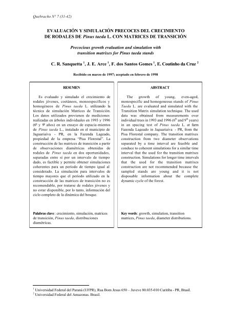
1999, son presentadas en las Figuras 2, 3, 4, 5 y 6, para los 5 tratamientos respectivamente. Las
Figuras 2 a 6 muestran una armonía propia de la dinámica de un proceso biológico, donde las
medidas de posición (media, moda) aumentan con el tiempo, junto con el aumento de las medidas
de dispersión (Figuras 4 y 6). Las pequeñas discrepancias observadas en las Figuras 2, 3 y 5
podrían ser resultado del hecho de estar trabajando con muestras pequeñas, rodales jóvenes y
no disponer de información del ciclo completo de la dinámica del bosque.
Las matrices seleccionadas para los 5 tratamientos son presentadas en las Tablas 1, 2, 3, 4 y
5. En las matrices pueden ser observadas algunas anomalías, una vez que las probabilidades pf1
y pf2 de la matriz de transición del tratamiento 1 tienen valor 1 (100%) (Tabla 1). Esto quiere
decir que todos los árboles de estas clases diamétricas permanecerán en sus respectivas clases,
sin existir transición para las clases siguientes. En la matriz de transición del tratamiento 2, el
valor de la probabilidad de que los árboles de la clase diamétrica 2 se mueran (pm2) tiene valor 1
(100%), diciendo que todos los árboles de esta clase diamétrica, morirán en el siguiente período
de simulación de tres años (Tabla 2). La misma observación puede ser hecha para las pm1 de
las matrices de transición de los tratamientos 3 y 4 (Tablas 3 y 4).

38 Revista de Ciencias Forestales – Quebracho N° 7 – Junio 1999
Figura 2
Tratamiento 1 - Clases de DAP de 2 cm.
Frecuencias [1/ha]
1400
1200
1000
800
600
400
200
0
1993
1996
1999
0 10 20 30 40 50
DAP[cm]
Figura 4
Tratamiento 3 - Clases de DAP de 3 cm.
Frecuencias [1/ha]
800
700
600
500
400
300
200
100
0
1993
Figura 6
Frecuencias [1/ha]
1996
600
500
400
300
200
100
0
1999
0 10 20 30 40
DAP[cm]
Tratamiento 5 - Clases de DAP de 4 cm.
1993
Figura 3
1996
1999
0 10 20 30 40
DAP[cm]
Tratamiento 2 - Clases de DAP de 3 cm.
Debido a la precocidad de la evaluación las probabilidades de transición disponibles a partir de los
datos observados corresponden solamente a las primeras clases diamétricas. En el tratamiento 1, las
probabilidades de transición fueron observadas hasta la clase diamétrica de 16-8 cm, en los tratamientos 2,
3 y 4, hasta la clase diamétrica de 18-21 cm, y en el tratamiento 5 hasta la clase diamétrica de 20-24 cm. En
consecuencia fue necesario asumir que las últimas probabilidades de transición observadas para los 5
tratamientos se mantienen constantes para todas las clases subsecuentes. De esta manera se satisface el
requisito de que la suma de las probabilidades de todas las líneas de la matriz de transición debe ser igual a
1: caso contrario se “perderían” árboles durante la simulación.
Frecuencias [1/ha]
1200
1000
800
600
400
200
0
1993
1996
1999
0 10 20 30 40
DAP[cm]
Figura 5
Tratamiento 4 - Clases de DAP de 3 cm.
Frecuencias [1/ha]
600
500
400
300
200
100
1993
1996
0
0 10 20 30 40
DAP[cm]
1999

Sanquetta et al.: Evaluación y simulación... 39
Tabla 1: Matriz de transición para el Tratamiento 1 a partir de clases diamétricas de 2 cm.
Muertas
0
0
0.50
0.08
0.03
0
0
0
0
0
0
0
0
0
0
0
0
0
0
0
1.00
38-40
-
-
-
-
-
-
-
-
-
-
-
-
-
-
-
-
0.33
0.67
1.00
1.00
-
36-38
-
-
-
-
-
-
-
-
-
-
-
-
-
-
-
0.33
0.33
0.33
0
-
-
34-36
-
-
-
-
-
-
-
-
-
-
-
-
-
-
0.33
0.33
0.33
0
-
-
-
32-34
-
-
-
-
-
-
-
-
-
-
-
-
-
0.33
0.33
0.33
0
-
-
-
-
30-32
-
-
-
-
-
-
-
-
-
-
-
-
0.33
0.33
0.33
0
-
-
-
-
-
28-30
-
-
-
-
-
-
-
-
-
-
-
0.33
0.33
0.33
0
-
-
-
-
-
-
26-28
-
-
-
-
-
-
-
-
-
-
0.33
0.33
0.33
0
-
-
-
-
-
-
-
24-26
-
-
-
-
-
-
-
-
-
0.33
0.33
0.33
0
-
-
-
-
-
-
-
-
22-24
-
-
-
-
-
-
-
-
0.33
0.33
0.33
0
-
-
-
-
-
-
-
-
-
20-22
-
-
-
-
-
-
-
0.06
0.33
0.33
0
-
-
-
-
-
-
-
-
-
-
18-20
-
-
-
-
-
-
0.01
0.24
0.33
0
-
-
-
-
-
-
-
-
-
-
-
16-18
-
-
-
-
-
0.01
0.28
0.67
0
-
-
-
-
-
-
-
-
-
-
-
-
14-16
-
-
-
-
0
0.24
0.65
0.03
-
-
-
-
-
-
-
-
-
-
-
-
-
12-14
-
-
-
0
0.12
0.61
0.06
-
-
-
-
-
-
-
-
-
-
-
-
-
-
10-12
-
-
0
0
0.51
0.14
-
-
-
-
-
-
-
-
-
-
-
-
-
-
-
8-10
-
0
0
0.36
0.34
-
-
-
-
-
-
-
-
-
-
-
-
-
-
-
-
6-8
0
0
0.25
0.56
-
-
-
-
-
-
-
-
-
-
-
-
-
-
-
-
-
4-6
0
0
0.25
-
-
-
-
-
-
-
-
-
-
-
-
-
-
-
-
-
-
2-4
0
1.00
-
-
-
-
-
-
-
-
-
-
-
-
-
-
-
-
-
-
-
>0-2
1.00
-
-
-
-
-
-
-
-
-
-
-
-
-
-
-
-
-
-
-
-
>0-2
2-4
4-6
6-8
8-10
10-12
12-14
14-16
16-18
18-20
20-22
22-24
24-26
26-28
28-30
30-32
32-34
34-36
36-38
38-40
Muertas

40 Revista de Ciencias Forestales – Quebracho N° 7 – Junio 1999
Tabla 2: Matriz de transición para el Tratamiento 2 a partir de clases diamétricas de 3 cm.
>0-3 3-6 6-9 9-12 12-15 15-18 18-21 21-24 24-27 27-30 30-33 33-36 36-39 Muertas
>0-3 1,00 0 0 0 - - - - - - - - - 0
3-6 - 0 0 0 0 - - - - - - - - 1,00
6-9 - - 0,60 0,40 0 0 - - - - - - - 0
9-12 - - - 0,21 0,74 0,05 0 - - - - - - 0
12-15 - - - - 0,19 0,61 0,19 0,01 - - - - - 0
15-18 - - - - - 0,06 0,65 0,29 0 - - - - 0
18-21 - - - - - - 0 1,00 0 0 - - - 0
21-24 - - - - - - - 0 1,00 0 0 - - 0
24-27 - - - - - - - - 0 1,00 0 0 - 0
27-30 - - - - - - - - - 0 1,00 0 0 0
30-33 - - - - - - - - - - 0 1,00 0 0
33-36 - - - - - - - - - - - 0 1,00 0
36-39 - - - - - - - - - - - - 1,00 0
Muertas - - - - - - - - - - - - - 1,00
Tabla 3: Matriz de transición para el Tratamiento 3 a partir de clases diamétricas de 3 cm.
>0-3 3-6 6-9 9-12 12-15 15-18 18-21 21-24 24-27 27-30 30-33 33-36 36-39 Muertas
>0-3 0 0 0 0 - - - - - - - - - 1,00
3-6 - 0,25 0,25 0 0 - - - - - - - - 0,50
6-9 - - 0 1,00 0 0 - - - - - - - 0
9-12 - - - 0,11 0,59 0,30 0 - - - - - - 0
12-15 - - - - 0,07 0,57 0,35 0,01 - - - - - 0
15-18 - - - - - 0 0,65 0,35 0 - - - - 0
18-21 - - - - - - 0 0,50 0,50 0 - - - 0
21-24 - - - - - - - 0 0,50 0,50 0 - - 0
24-27 - - - - - - - - 0 0,50 0,50 0 - 0
27-30 - - - - - - - - - 0 0,50 0,50 0 0
30-33 - - - - - - - - - - 0 0,50 0,50 0
33-36 - - - - - - - - - - - 0 1,00 0
36-39 - - - - - - - - - - - - 1,00 0
Muertas - - - - - - - - - - - - - 1,00
Tabla 4: Matriz de transición para el Tratamiento 4 a partir de clases diamétricas de 3 cm.
>0-3 3-6 6-9 9-12 12-15 15-18 18-21 21-24 24-27 27-30 30-33 33-36 36-39 Muertas
>0-3 0 0 0 0 - - - - - - - - - 1,00
3-6 - 0 0,20 0 0 - - - - - - - - 0,80
6-9 - - 0,25 0,50 0,13 0 - - - - - - - 0,13
9-12 - - - 0,04 0,67 0,30 0 - - - - - - 0
12-15 - - - - 0,05 0,32 0,58 0,06 - - - - - 0
15-18 - - - - - 0,01 0,49 0,47 0,03 - - - - 0
18-21 - - - - - - 0 0,50 0,50 0 - - - 0
21-24 - - - - - - - 0 0,50 0,50 0 - - 0
24-27 - - - - - - - - 0 0,50 0,50 0 - 0
27-30 - - - - - - - - - 0 0,50 0,50 0 0
30-33 - - - - - - - - - - 0 0,50 0,50 0
33-36 - - - - - - - - - - - 0 1,00 0
36-39 - - - - - - - - - - - - 1,00 0
Muertas - - - - - - - - - - - - - 1,00
Tabla 5: Matriz de transición para el Tratamiento 5 a partir de clases diamétricas de 4 cm.
>0-4 4-8 8-12 12-16 16-20 20-24 24-28 28-32 32-36 36-40 Muertas
>0-4 1,00 0 0 0 - - - - - - 0
4-8 - 0 1,00 0 0 - - - - - 0
8-12 - - 0,08 0,75 0,17 0 - - - - 0
12-16 - - - 0,03 0,51 0,47 0 - - - 0
16-20 - - - - 0 0,81 0,19 0 - - 0
20-24 - - - - - 0 0,71 0,29 0 - 0
24-28 - - - - - - 0 0,71 0,29 0 0
28-32 - - - - - - - 0 0,71 0,29 0
32-36 - - - - - - - - 0 1,00 0
36-40 - - - - - - - - - 1,00 0
Muertas - - - - - - - - - - 1,00

Sanquetta et al.: Evaluación y simulación... 41
Las probabilidades de transición contenidas en las matrices (Tablas 1 a 5) fueron calculadas
a partir de datos tomados en remediciones. En general, si las clases dia métricas fuesen bien
determinadas (amplitud adecuada), las probabilidades de crecimiento pueden ser estimadas de
manera consistente, pero para mayor seguridad es necesaria una evaluación continua de estas
probabilidades a lo largo de todo el turno. El problema es más serio en el caso de las
probabilidades de mortalidad, en virtud de ser éste un evento considerado raro y episódico en
rodales comerciales. Por lo tanto, la estimación de las probabilidades de mortalidad es más
problemática en rodales jóvenes, como los estudiados en esta investigación, considerando que los
procesos de competencia aún no se han intensificado. Esto provoca estimaciones inconsistentes
de las probabilidades de mortalidad, generando anomalías en las proyecciones, conforme fue
discutido previamente en el texto. Esto representa una limitación al empleo del modelo matricial
para proyecciones de largo plazo, principalmente cuando los datos provienen de rodales jóvenes.
Otro aspecto cuestionable de la simulación con matrices de transición es la suposición de que
las probabilidades, una vez calculadas e insertadas en la matriz de transición, permanecerán
constantes a lo largo de toda la vida del bosque. Este aspecto particular, entre otras desventajas
del modelo, fue muy debatido entre los investigadores que trabajaron con matrices de transición,
como por ejemplo Bruner y Moser (1973), Enright y Ogden (1979). Sin embargo, esta es una
propiedad intrínseca de este tipo de modelo, y no es susceptible a mejoras. Alder (1980) detalla
otras limitaciones inherentes a las matrices de transición.
Infelizmente existen pocos estudios sobre modelos de simulación para proyección de la
producción forestal de rodales de Pinus taeda en el Brasil (Oliveira, 1995), que permitan
comparar los resultados presentados en este artículo. A pesar de ello, las figuras generadas por
simulación en el presente trabajo se han mostrado, en forma general, coherentes con la realidad
de las evoluciones diamétricas comúnmente observadas en las plantaciones forestales de Pinus.
5. CONCLUSIONES Y RECOMENDACIONES
La construcción de matrices de transición a partir de observaciones diamétricas obtenidas de
rodales jóvenes, coetáneos, monoespecíficos y homogéneos de Pinus taeda en dos
oportunidades, separadas entre sí por un intervalo de tiempo dado, es factible y permite obtener
simulaciones coherentes para un período igual al período de tiempo considerado. En el caso
analizado las observaciones fueron realizadas en el 6 o y 9 o años (1993 y 1996), y permitieron
simular las frecuencias diamétricas para el 12 o año (1999). Las simulaciones obtenidas muestran
una armonía propia de la dinámica de un proceso biológico, donde las medidas de posición
(media, moda) aumentan con el tiempo, junto con el aumento de las medidas de dispersión. La
simulación para intervalos de tiempo mayores que el período de tiempo considerado para la
construcción de las matrices de transición no es aconsejable, por tratarse de rodales jóvenes y
no estar disponible, por lo tanto, información del ciclo completo de la dinámica del bosque.
Sería recomendable proseguir con las observaciones y mediciones del bosque hasta el final
del ciclo, tanto para validar los resultados obtenidos con las simulaciones presentadas en este
estudio como para calibrar y construir matrices de transición para períodos y edades diferentes.
De esta manera la simulación de las distribuciones diamétricas se tornaría más dinámica
utilizando sucesivamente varias matrices de transición hasta alcanzar el final del ciclo, conforme
argumentado por Alder (1980). La calibración y retroalimentación constantes con datos
provenientes de plantaciones comerciales es requisito fundamental de cualquier modelo de
simulación forestal.

42 Revista de Ciencias Forestales – Quebracho N° 7 – Junio 1999
AGRADECIMIENTOS
Los autores desean agradecer de modo muy especial a la empresa Pisa Florestal por haber
facilitado gentilmente los datos utilizados en el presente trabajo, y a las personas Walquiria
Pizatto, Jeferson Wendling, Zenóbio A. G. P. da Gama e Silva, Ruth Loch y Alexandra C. P. S.
Bartosczek.
Nota del Comité editor: El autor también presento una rutina de trabajo programada para la
obtención de matrices de transición, la cual no es publicada por razones de espacio.
REFERENCIAS
Alder, D. 1980. Estimación del volumen forestal y predicción del rendimiento con especial referencia a los
trópicos. Tomo II: Predicción del rendimiento. FAO 22/2. Italia. 118 p.
Bruner, H. D. & J. W. Moser Jr. 1973. A Markov chain approach to the prediction of diameter distributions
in uneven-aged forest stands. Canadian Journal Forest Research 3, 409-417.
Buongiorno, J. & B. R. Michie 1980. A matrix model for uneven-aged forest management. Forest Science
26: 609-625. U.S.A.
Clutter, J.L.; J. C. Fortson; L. V. Pienaar; G. H. Brister. & R. L. Bailey 1983. Timber management: a
quantitative approach. Ed. John Wiley & sons. New York, USA
Daniel, P.W.; U. E. Helms y F. S. Baker, 1982. Principios de silvicultura. Ed Mc Graw Hill. México. 492p.
Davis, L.S. & K. N. Johnson 1987. Forest management. Mc Graw-Hill Book. USA. 790p.
Enright, N. & J. Ogden 1979. Applications of transition matrix models in forest dynamics: Araucaria in
Papua New Guinea and Nothofagus in New Zealand. Australian Journal of Ecology, N° 4, p. 3-
23.
Harrison, T. P. & B. R. Michie 1985. A generalized approach to the use of matrix growth models. Forest
Science, v. 31, N° 4, p. 850-856.
Hoyos, A. 1980. Processos estocásticos e previsão. In: 4 o Simpósio Nacional de Probabilidade e
Estatística. Rio de Janeiro, 21 a 25 de julho de 1980.
Leak, W. B. 1965. The J-shaped probability distribution. Forest Science, v. 11, N° 4, p. 405-409.
Lowell, K. E. & R. J Mitchell 1987. Modeling growth and mortality probabilistically using logistic
regression. USDA Forest Service NC GTR, St. Paul, p. 708-715.
Mendoza, G. A. & A. Setyarso 1986. A transition matrix forest growth model for evaluating alternative
harvesting schemes in Indonesia. Forest Ecology and Management., N° 15, p. 219-228.
Oliveira, E. B. 1995. Um sistema computadorizado de prognose do crescimento e produção de Pinus taeda
L., com critérios quantitativos para a avaliação técnica e econômica de regimes de manejo. Tesis
(Doctorado en Manejo Forestal), Universidad Federal del Paraná.134p.
Roberts, M. R. & A. J Hruska 1986. Predicting diameter distributions: a test of the stationary Markov
model. Canadian Journal Forest Research, N° 16, p. 130-135.
Sanquetta, C. R. 1996. Fundamentos biométricos dos modelos de simulação florestal. FUPEF - Série
didática N° 8. Curitiba (PR), Brasil.
Spurr, S. H. 1952. Forest inventory. The Ronald Press Company. New York, USA. 476p.