Tema 2: Introducción al control robusto - Universidad Pública de ...

Universidad Pública de Navarra
Tema 2 – Introducción al control robusto
Master energías renovables - Master IMAC
Ingeniería de control robusto
Tema 2- Introducción al control robusto
Jorge Elso Torralba
Dpto. automática y computación
Tema 2 – Introducción al control robusto
La necesidad de realimentación
Realimentación
Control robusto
Control 2 DOF
Sensibilidad
Limitaciones
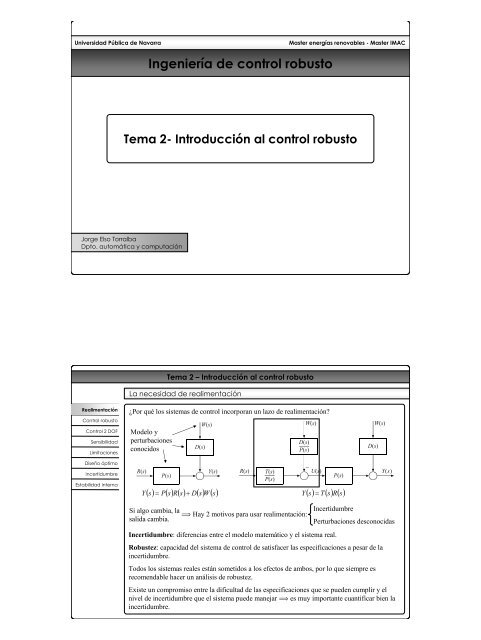
¿Por qué los sistemas de control incorporan un lazo de realimentación?
W(s)
W(s)
Modelo y
perturbaciones
D(s)
conocidos
D(s)
P(s)
D(s)
W(s)
Diseño óptimo
Incertidumbre
Estabilidad interna
R(s)
Y(s)
P(s)
() s = P() s R() s D( s) W ( s)
Y +
R(s)
T(s)
P(s)
- U(s)
P(s)
( s) T ( s) R( s)
Y =
Y(s)
Si algo cambia, la
salida cambia.
ï Hay 2 motivos para usar realimentación:
Incertidumbre
Perturbaciones desconocidas
Incertidumbre: diferencias entre el modelo matemático y el sistema real.
Robustez: capacidad del sistema de control de satisfacer las especificaciones a pesar de la
incertidumbre.
Todos los sistemas reales están sometidos a los efectos de ambos, por lo que siempre es
recomendable hacer un análisis de robustez.
Existe un compromiso entre la dificultad de las especificaciones que se pueden cumplir y el
nivel de incertidumbre que el sistema puede manejar ï es muy importante cuantificar bien la
incertidumbre.

Tema 2 – Introducción al control robusto
El problema de control robusto
Realimentación
Control robusto
Control 2 DOF
Sensibilidad
Limitaciones
Diseño óptimo
Incertidumbre
Estabilidad interna
El problema general de control automático es
w
r
u
y
controlador
planta
v
sensor
n
Dado un sistema o planta, un conjunto de
señales de salida medidas v, determinar
qué acciones de control u deben realizarse
para que las variables controladas y sigan
lo mejor posible a las señales de referencia
r, a pesar de la influencia de perturbaciones
w y ruido de medida n.
‣ El sistema puede estar modelado por ecuaciones diferenciales lineales, no lineales, de
parámetros concentrados o distribuidos, etc.
‣ Por otro lado, pueden existir no linealidades tipo saturación, zona muerta, cuantización, etc,
tanto en los sensores como en los actuadores (que se consideran parte de la planta).
‣Pueden ser establecidos límites en las acciones de control permitidas.
‣El modelo disponible no describe perfectamente al sistema, y además éste varía con el tiempo.
Objetivo del control robusto: hacer que todas las posibles salidas de las diferentes plantas dentro
de la incertidumbre pertenezcan a un conjunto de salidas aceptables.
El problema de control robusto se suele afrontar desde los métodos de respuesta frecuencial.
Tema 2 – Introducción al control robusto
Sistemas de control con dos grados de libertad
Realimentación
Control robusto
Control 2 DOF
Sensibilidad
Ejemplos de esquemas de dos grados de libertad:
1
R(s) + E(s) 1 +
U(s) Y(s)
K
P(s)
R(s) + E(s) 1 + +
TIs
U(s) Y(s)
-
K
P(s)
TIs
-
+ +
Limitaciones
Diseño óptimo
TDs
PI-D
1 TDs
I-PD
Incertidumbre
C 2(s)
Estabilidad interna
+
-
C 1(s)
+ +
H(s)
P (s)
Feed-forward
Todos los esquemas se
pueden reducir al general
Esquema de dos grados de libertad general:
Controlador de realimentación: reduce de los efectos
de las perturbaciones y de la incertidumbre
W(s)
D(s)
Prefiltro: acomoda la
señal de entrada para
mejorar el seguimiento
de referencia
R(s)
F(s)
E(s)
-
C(s)
U(s)
H(s)
P(s)
Y(s)
N(s)
El controlador ideal para rechazo de perturbaciones es distinto del controlador ideal para
seguimiento de referencia ï se recurre a un esquema de dos grados de libertad.

Tema 2 – Introducción al control robusto
La función de sensibilidad y la realimentación
Realimentación
Control robusto
Control 2 DOF
Sensibilidad
Limitaciones
Diseño óptimo
Incertidumbre
Estabilidad interna
¿Cómo logra la realimentación atenuar los efectos de la incertidumbre y las perturbaciones?
La función de sensibilidad nos da la respuesta:
∆F()
s
Sistema formado
por la interconexión
V(s)
F
()
() s
S s =
A(s)
de funciones de
∆V
() s
transferencia, una de
... ... Y(s)
V () s
las cuales cambia:
C(s)
B(s)
V
()
() s dF s
S F , V s =
F s dV s
Aplicándola sobre el lazo abierto y el lazo cerrado siguientes
R(s)
R(s)
-
P(s)
Y(s)
P(s)
H(s)
Y(s)
⇒ S
⇒ S
( s) 1
T R
() s
, P =
=
T , P R 1 +
1
P
() s H () s
⎧V
⎪
⇒ ⎨F
⎪
⎩
( s) = P( s)
Y
()
() s
s =
R()
s
= T
R
() s
()
()
()
El lazo cerrado
proporciona una
reducción de la
sensibilidad frente a
los cambios en la
planta con un factor
1
1+ P s H s
() ()
Tema 2 – Introducción al control robusto
Sensibilidad, lazo abierto y sensibilidad complementaria
Realimentación
Control robusto
Control 2 DOF
Sensibilidad
Limitaciones
Diseño óptimo
Incertidumbre
Estabilidad interna
La función de sensibilidad de un sistema con realimentación se refiere a la sensibilidad de la
función referencia-salida ente variaciones en la planta.
En un esquema 2 DOF general dicha función es
S
() s
= 1
1 + P
() s C() s H () s
La función de lazo abierto es el producto de todas las funciones de transferencia situadas
dentro del lazo:
() s P() s C() s H ( s)
L =
fl De modo general, la función de sensibilidad se define como
S
() s
= ˆ
1
1 + L
() s
La función sensibilidad complementaria se define de modo similar:
() s
L()
s
L
T () s = ˆ 1+
El término “complementaria” proviene de la relación
S
() s + T() s = 1
que es una de las restricciones fundamentales de todo sistema de control.

Tema 2 – Introducción al control robusto
Sensibilidad, lazo abierto y sensibilidad complementaria
Realimentación
Control robusto
Control 2 DOF
Sensibilidad
La señal de salida de un
sistema 2DOF viene dada
por la función
R(s)
F(s)
E(s)
-
C(s)
W(s)
U(s)
D(s)
P(s)
Y(s)
Limitaciones
Diseño óptimo
Incertidumbre
Estabilidad interna
Y
Y
() s
=
1+
P
D()
s
() s C() s H () s
W
() s
P
+
1+
( s) = T ( s) W ( s) + T ( s) R( s) −T
( s) N( s)
W
R
N
( s) C( s) F( s)
R()
s
P() s C() s H () s
P
−
1+
H(s)
( s) C( s) H ( s)
P() s C() s H () s
fl hay tres funciones de transferencia en lazo cerrado, que comparten el denominador 1+L(s):
N
() s
N(s)
Esta ecuación puede reescribirse en términos de las sensibilidades:
Y
() s = S() s D() s W () s + T()
s
Conclusiones:
( s)
R() s −T() s N()
s
() s
F
H
La transición entre
estos dos
determina la
estabilidad.
1. La manera de disminuir el efecto de las perturbaciones es reducir S(s).
2. Si se consigue T(s)º1, se puede ajustar F(s) para tener el T R (s) deseado.
3. La manera de disminuir el efecto del ruido es reducir T(s).
↑ L( jω)
↓ L( jω)
Tema 2 – Introducción al control robusto
Limitaciones: Integral de sensibilidad
Realimentación
Control robusto
Control 2 DOF
Sensibilidad
Limitaciones
Diseño óptimo
Incertidumbre
Estabilidad interna
Para cualquier sistema de fase mínima en el que hay al menos dos polos más que ceros en lazo
abierto (la mayoría de los casos reales son así), se cumple la siguiente integral:
∫ ∞ ln S( jω) dω = 0
0
1
0
-1
-2
-3
ln|S(jw)|
Realimentación
negativa
Realimentación
positiva
5
0
-5
-10
-15
-20
-25
|S(jw)| (dB)
-4
-30
-35
-5
-40
0 1 2 3 4 5 6 7 8 9 10 10 -2 10 -1 10 0 10 1 10 2
Frequency (rad/sec)
Frequency (rad/sec)
Se conoce a 1/S(jw) = 1+L(jw) como función de realimentación, y la integral es la misma para
ella. Esto nos lleva a distinguir entre áreas de realimentación negativa y positiva.
Ambas son iguales fl si se reduce el efecto de perturbaciones e incertidumbre en una zona,
entonces existe otra región en la que dicho efecto se incrementa.
La realimentación positiva se concentra cerca de la frecuencia de cruce de ganancia.

Tema 2 – Introducción al control robusto
El coste de la realimentación
Realimentación
Control robusto
Control 2 DOF
Sensibilidad
Limitaciones
Diseño óptimo
Incertidumbre
Estabilidad interna
C() s H () s −1
=
() s C() s H () s P()
s
−
L
T UN () s =
1+
P
1+
L
1
( s)
L()
s
3 rangos:
( jω)
>> 1
( jω)
≈ 1
( jω) > 1⇒
TUN
( jω)
≈
( jω)

Tema 2 – Introducción al control robusto
Origen de la incertidumbre
Realimentación
Control robusto
Control 2 DOF
Sensibilidad
Limitaciones
Diseño óptimo
Incertidumbre
El trabajo de análisis y diseño del ingeniero se realiza sobre el modelo del sistema.
El modelo nunca describe
completamente el comportamiento
del sistema ï hay incertidumbre.
Incapacidad de llegar a un
modelo perfecto
Eliminación deliberada de
aspectos del modelo
Estabilidad interna
Tarea del diseñador
Definir el conjunto de todas las
posibles plantas que pueden describir
al sistema en un momento dado
¿Qué sabemos sobre lo
que no conocemos?
Fuentes de incertidumbre:
1. Medición de los parámetros físicos
2. Cambio en los parámetros físicos, por condiciones ambientales, envejecimiento, …
3. Linealización de la planta
4. Sensores y actuadores
5. Altas frecuencias ï estructura y orden del modelo desconocidos
6. Dinámica ignorada para simplificar el diseño
Tema 2 – Introducción al control robusto
Tipos de incertidumbre
Realimentación
Control robusto
Control 2 DOF
Sensibilidad
Limitaciones
Diseño óptimo
Incertidumbre
Estabilidad interna
De acuerdo con su origen, la incertidumbre se puede separar en dos categorías
1) Incertidumbre paramétrica o estructurada.
‣ Estructura conocida
‣ Parámetros pertenecientes a intervalos
P
m
( α , s) , α ∈ Ω ∈
( α , s) ∈ P( α s)
Cada α i ∈ Ω genera un P i ,
z
z
W
z
a
wn
wn
wn
Ejemplo
P
n
( α,
s) =
;
k ∈
2
2
kω
n
2
n
s + 2ζω
s + ω
[ k, k] ; ζ ∈[ ζ , ζ ];
ω ∈[ ω , ω ]
n
n
n
k
k
Otra forma de presentar incertidumbre estructurada es simplemente dar un conjunto de posibles
plantas, sin definir explícitamente intervalos de variación de los parámetros.
Valor de referencia de los parámetros
Planta nominal P 0 (s)
Las demás plantas se interpretan como
desviaciones respecto a la nominal.

Tema 2 – Introducción al control robusto
Tipos de incertidumbre
Realimentación
Control robusto
Control 2 DOF
Sensibilidad
Limitaciones
2) Incertidumbre no paramétrica o no estructurada.
P(s)
WI(s) DI(s)
P
Planta nominal
( s) = P ( s) ( 1+ W ( s) ∆ ( s)
)
0
I
I
Diseño óptimo
P0(s)
Incertidumbre
Estabilidad interna
Incertidumbre multiplicativa
Función de peso:
representa el nivel
de incertidumbre
en cada frecuencia
Cualquier función
que cumple
( jω) ≤ ∀ω
∆ 1
I
‣ Es más difícil de cuantificar
‣ Lleva a resultados más conservadores
‣ Es la única que se puede emplear en altas frecuencias
¿Cuál de ellas usar? Depende de la técnica de control robusto que utilicemos:
QFT ö Permite el uso de ambas
H , m análisis, etc ö Incertidumbre no paramétrica
Tema 2 – Introducción al control robusto
Estabilidad y estabilidad interna
Realimentación
Control robusto
Control 2 DOF
Sensibilidad
Limitaciones
Diseño óptimo
Incertidumbre
Estabilidad interna
Sabemos que la estabilidad de un sistema viene dada por la posición de los ceros de la ecuación
característica, que es el denominador de todas las funciones de transferencia de lazo cerrado.
Por ejemplo, la sensibilidad complementaria: T
Criterios de
estabilidad
‣Routh-Hurwitz
‣ Lugar de raíces
() s
‣ Criterio de Nyquist ö MG, MF
P
= 1+
( s) C( s) H ( s)
P() s C() s H () s
Nos dicen si hay polos de T(s)
en el RHP, basándose en L(s)
Pero esos criterios no son suficientes:
R(s)
T
-
1
= s + 2
1
(s-1)
() s ;
U(s) (s-1) Y(s) 1. La cancelación perfecta es
(s+1)
U
R
( s)
s + 1
=
() s ( s −1)( s + 2)
imposible, pero aunque así fuera,
2. u(t) crece sin cota, lo que en la
práctica satura los actuadores.
Es un problema de estabilidad interna: presencia de modos ocultos inestables.
Un sistema es internamente estable si cumple el criterio de estabilidad de Nyquist, y además,
no se producen cancelaciones cero-polo en el RHP entre ninguno de los elementos de L(s).
Si lo anterior se cumple para todos los miembros de P, hablamos de estabilidad robusta.