elementos de la teoria de tensiones y deformaciones - unne
elementos de la teoria de tensiones y deformaciones - unne
elementos de la teoria de tensiones y deformaciones - unne

Create successful ePaper yourself
Turn your PDF publications into a flip-book with our unique Google optimized e-Paper software.
ESTABILIDAD II<br />
CAPITULO III: ELEMENTOS DE LA TEORIA DE TENSIONES Y DEFORMACIONES<br />
3<br />
ELEMENTOS DE LA TEORIA DE<br />
TENSIONES Y DEFORMACIONES<br />
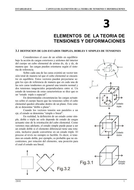
3.1 DEFINICION DE LOS ESTADOS TRIPLES, DOBLES Y SIMPLES DE TENSIONES<br />
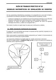
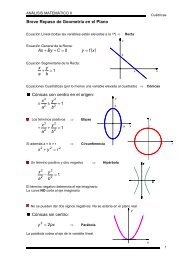
Consi<strong>de</strong>remos el caso <strong>de</strong> un sólido en equilibrio<br />
bajo <strong>la</strong> acción <strong>de</strong> cargas exteriores y aislemos <strong>de</strong>l interior<br />
<strong>de</strong>l cuerpo un cubo elemental <strong>de</strong> aristas dx, dy y dz, <strong>de</strong><br />
manera que <strong>la</strong>s cargas pue<strong>de</strong>n orientarse según el sistema<br />
<strong>de</strong> referencia.<br />
Sobre cada una <strong>de</strong> <strong>la</strong>s caras existirá un vector tensión<br />
total <strong>de</strong> manera tal que el cubo elemental se encuentre<br />
en equilibrio. Estos vectores pue<strong>de</strong>n proyectarse según<br />
los ejes <strong>de</strong> referencia <strong>de</strong> manera que en cada una <strong>de</strong><br />
<strong>la</strong>s seis caras tendremos en general una tensión normal y<br />
dos <strong>tensiones</strong> tangenciales perpendicu<strong>la</strong>res entre si. Un<br />
estado <strong>de</strong> <strong>tensiones</strong> <strong>de</strong> estas características se dice que es<br />
un “estado triple o espacial”.<br />
En <strong>de</strong>terminadas circunstancias <strong>la</strong>s cargas actuantes<br />
sobre el cuerpo hacen que <strong>la</strong>s <strong>tensiones</strong> sobre el cubo<br />
elemental que<strong>de</strong>n ubicadas <strong>de</strong>ntro <strong>de</strong> un p<strong>la</strong>no. Este estado<br />
se <strong>de</strong>nomina “doble o p<strong>la</strong>no”.<br />
Cuando los vectores tensión son paralelos a un<br />
eje, el estado se <strong>de</strong>nomina “simple o lineal”.<br />
En realidad, <strong>la</strong> <strong>de</strong>finición <strong>de</strong> un estado como simple,<br />
doble o triple no solo <strong>de</strong>pen<strong>de</strong> <strong>de</strong> estado <strong>de</strong> cargas<br />
actuante sino <strong>de</strong> <strong>la</strong> orientación <strong>de</strong>l cubo elemental. Como<br />
veremos mas a<strong>de</strong><strong>la</strong>nte, el estado simple pue<strong>de</strong> pasar a ser<br />
un estado doble si el elemento diferencial tiene una rotación,<br />
inclusive pue<strong>de</strong> convertirse en un estado triple. El<br />
proceso al revés no siempre es factible. Es <strong>de</strong>cir, si tenemos<br />
un estado doble, por ejemplo, es probable que no encontremos,<br />
por rotación <strong>de</strong>l elemento, una posición para<br />
el cual el estado sea lineal.<br />
/2010 1
ESTABILIDAD II<br />
CAPITULO III: ELEMENTOS DE LA TEORIA DE TENSIONES Y DEFORMACIONES<br />
Para po<strong>de</strong>r enten<strong>de</strong>rnos con c<strong>la</strong>ridad al referirnos a <strong>la</strong>s <strong>tensiones</strong>, vamos a establecer ciertas<br />
convenciones:<br />
i : el subíndice i indicará al eje respecto <strong>de</strong>l cual <strong>la</strong>s <strong>tensiones</strong> normales son parale<strong>la</strong>s ( x , y , z ).<br />
Serán positivas cuando produzcan tracción.<br />
ij : el subíndice i indicará el vector normal al p<strong>la</strong>no don<strong>de</strong> actúan <strong>la</strong>s <strong>tensiones</strong> tangenciales, y el subíndice<br />
j indicará el eje al que resultan parale<strong>la</strong>s ( xy , xz , yz , yx , zx , zy ).<br />
Tanto <strong>la</strong>s <strong>tensiones</strong> normales como <strong>la</strong>s tangenciales varían punto a punto en el interior <strong>de</strong> un<br />
cuerpo, por lo tanto, <strong>de</strong>bemos tener presente que <strong>la</strong>s <strong>tensiones</strong> quedan expresadas como funciones:<br />
= (x,y,z)<br />
= (x,y,z)<br />
3.2 EQUILIBRIO DE UN PRISMA ELEMENTAL<br />
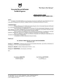
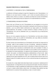
Consi<strong>de</strong>remos, como en <strong>la</strong> figura 3.3, un punto A correspondiente a un sólido sujeto a <strong>tensiones</strong>,<br />
punto que hacemos coincidir con el origen <strong>de</strong> coor<strong>de</strong>nadas; y tres p<strong>la</strong>nos perpendicu<strong>la</strong>res que pasan<br />
por el punto, coinci<strong>de</strong>ntes con los p<strong>la</strong>nos coor<strong>de</strong>nados. Supongamos a<strong>de</strong>más un segundo punto B<br />
<strong>de</strong>l mismo sólido, <strong>de</strong> coor<strong>de</strong>nadas dx, dy y dz..<br />
Admitiremos que <strong>la</strong>s funciones que <strong>de</strong>finen <strong>la</strong>s <strong>tensiones</strong> en los puntos <strong>de</strong>l sólido son continuas<br />
y <strong>de</strong>rivables. Las <strong>tensiones</strong> que actúan en los p<strong>la</strong>nos que pasan por B pue<strong>de</strong>n <strong>de</strong>finirse como <strong>la</strong>s<br />
que actúan en los p<strong>la</strong>nos paralelos pasantes por A mas el correspondiente incremento. Así tendremos,<br />
σ<br />
x<br />
por ejemplo, <br />
x<br />
y <br />
x<br />
dx tomando como incremento el primer término <strong>de</strong>l <strong>de</strong>sarrollo en serie<br />
x<br />
<strong>de</strong> Taylor.<br />
/2010 2
ESTABILIDAD II<br />
CAPITULO III: ELEMENTOS DE LA TEORIA DE TENSIONES Y DEFORMACIONES<br />
El prisma elemental estará sometido a fuerzas actuantes en sus caras como consecuencia <strong>de</strong> <strong>la</strong>s<br />
<strong>tensiones</strong>, a<strong>de</strong>más existirá una fuerza <strong>de</strong> masa que supondremos aplicada en el baricentro. L<strong>la</strong>maremos<br />
X, Y, Z a <strong>la</strong>s componentes <strong>de</strong> dicha fuerza por unidad <strong>de</strong> volumen.<br />
Si p<strong>la</strong>nteamos el equilibrio <strong>de</strong>l prisma elemental tendremos:<br />
<br />
F<br />
x<br />
0<br />
<br />
<br />
<br />
<br />
x<br />
<br />
x <br />
dxdy<br />
dz <br />
x<br />
<br />
x<br />
<br />
dy dz <br />
<br />
zx<br />
<br />
<br />
z<br />
zx<br />
<br />
dzdx dy <br />
<br />
zx<br />
dx dy <br />
<br />
<br />
<br />
<br />
yx<br />
<br />
yx<br />
<br />
y<br />
<br />
dy<br />
dx dz <br />
<br />
yx<br />
dx dz X dx dy dz 0<br />
<br />
<br />
x<br />
x<br />
<br />
<br />
z<br />
zx<br />
<br />
yx<br />
<br />
y<br />
<br />
X<br />
dx dy dz 0<br />
<br />
<br />
x<br />
x<br />
<br />
<br />
yx<br />
y<br />
<br />
<br />
zx<br />
z<br />
X<br />
<br />
0<br />
Por F<br />
<br />
xy<br />
x<br />
y<br />
<br />
0 ; FZ<br />
0 , se obtiene<br />
<br />
y<br />
y<br />
zy<br />
<br />
z<br />
Y 0<br />
:<br />
ECUACIONES DIFERENCIALES<br />
DEL EQUILIBRIO<br />
(3.1)<br />
<br />
xz<br />
x<br />
<br />
<br />
yz<br />
y<br />
<br />
<br />
z<br />
z<br />
Z<br />
<br />
0<br />
Continuando con <strong>la</strong>s ecuaciones <strong>de</strong> momento, para lo cual suponemos tras<strong>la</strong>dada <strong>la</strong> terna <strong>de</strong><br />
ejes al baricentro <strong>de</strong>l elemento, tendremos:<br />
<br />
Mx 0<br />
<br />
<br />
<br />
<br />
- <br />
<br />
yz<br />
zy<br />
<br />
yz<br />
<br />
y<br />
<br />
zy<br />
<br />
z<br />
<br />
dy dx<br />
dz<br />
<br />
<br />
dzdx<br />
dy<br />
<br />
dy<br />
2<br />
dz<br />
2<br />
<br />
yz<br />
<br />
zy<br />
dx dz<br />
dx dy<br />
dy<br />
2<br />
dz<br />
2<br />
<br />
0<br />
Despreciando diferenciales <strong>de</strong> or<strong>de</strong>n superior nos queda:<br />
<br />
yz<br />
dx<br />
dy<br />
dz<br />
<br />
zy<br />
dx<br />
dy<br />
dz<br />
<br />
0<br />
<br />
<br />
yz<br />
<br />
<br />
zy<br />
(3.2)<br />
I<strong>de</strong>nticame<br />
nte<br />
<br />
<br />
My<br />
Mz<br />
0<br />
0<br />
<br />
<br />
<br />
<br />
xz<br />
xy<br />
<br />
<br />
<br />
<br />
zx<br />
yx<br />
<br />
xy<br />
<br />
<br />
yx<br />
<br />
xz<br />
<br />
<br />
zx<br />
<br />
yz<br />
<br />
<br />
zy<br />
/2010 3
ESTABILIDAD II<br />
CAPITULO III: ELEMENTOS DE LA TEORIA DE TENSIONES Y DEFORMACIONES<br />
Estas últimas ecuaciones reciben el nombre <strong>de</strong> “LEY DE CAUCHY o LEY DE RECIPRO-<br />
CIDAD DE LAS TENSIONES TANGENCIALES”, cuyo enunciado es: “En dos p<strong>la</strong>nos normales<br />
cualesquiera, cuya intersección <strong>de</strong>fine una arista, <strong>la</strong>s componentes normales a ésta <strong>de</strong> <strong>la</strong>s <strong>tensiones</strong><br />
tangenciales que actúan en dichos p<strong>la</strong>nos, son <strong>de</strong> igual intensidad y concurren o se alejan <strong>de</strong> <strong>la</strong> arista”.<br />
Las ecuaciones diferenciales <strong>de</strong>l equilibrio tienen nueve incógnitas, <strong>la</strong>s que consi<strong>de</strong>rando <strong>la</strong><br />
ley <strong>de</strong> Cauchy se reducen a seis. Ahora bien, siendo que sólo disponemos <strong>de</strong> tres ecuaciones, el número<br />
<strong>de</strong> incógnitas exce<strong>de</strong> el número <strong>de</strong> ecuaciones, con lo que concluimos que este problema resulta<br />
ESTATICAMENTE INDETERMINADO. Las ecuaciones que faltan pue<strong>de</strong>n obtenerse sólo si se estudian<br />
<strong>la</strong>s CONDICIONES DE DEFORMACION y se tienen en cuenta <strong>la</strong>s propieda<strong>de</strong>s físicas <strong>de</strong>l<br />
cuerpo dado (por ejemplo <strong>la</strong> ley <strong>de</strong> Hooke).<br />
La <strong>de</strong>terminación <strong>de</strong>l estado tensional <strong>de</strong> un cuerpo siempre resulta in<strong>de</strong>terminado por condición<br />
interna e implica <strong>la</strong> consi<strong>de</strong>ración <strong>de</strong> ecuaciones <strong>de</strong> compatibilidad, <strong>la</strong>s cuales establecen re<strong>la</strong>ciones<br />
entre <strong>la</strong>s <strong>de</strong>formaciones, en forma simi<strong>la</strong>r a como <strong>la</strong>s ecuaciones diferenciales <strong>de</strong>l equilibrio re<strong>la</strong>cionan<br />
a <strong>la</strong>s <strong>tensiones</strong> entre sí.<br />
Hay dos ciencias que tratan <strong>de</strong> resolver este problema:<br />
- La Teoría <strong>de</strong> <strong>la</strong> E<strong>la</strong>sticidad<br />
- La Resistencia <strong>de</strong> Materiales<br />
En <strong>la</strong> primera aparecen otras ecuaciones diferenciales aparte <strong>de</strong> <strong>la</strong>s <strong>de</strong> equilibrio, se agregan e-<br />
cuaciones <strong>de</strong> contorno y se trata <strong>de</strong> obtener <strong>la</strong> solución mediante <strong>la</strong> integración <strong>de</strong> <strong>la</strong>s ecuaciones diferenciales.<br />
El proceso es complejo y en muchos casos es muy difícil <strong>de</strong> encontrar <strong>la</strong> solución rigurosa<br />
<strong>de</strong>l problema, recurriendo a métodos numéricos. En el ámbito <strong>de</strong> <strong>la</strong> Resistencia <strong>de</strong> Materiales, en<br />
cambio, se hacen hipótesis aproximadas, aplicables a distintos casos particu<strong>la</strong>res, y que se verifican<br />
experimentalmente.<br />
Cuando resolvimos el problema <strong>de</strong> <strong>la</strong> solicitación normal, sin haberlo mencionado específicamente,<br />
hemos utilizado una ecuación <strong>de</strong> compatibilidad: <strong>la</strong> Ley <strong>de</strong> Bernoulli. En efecto, esta ley nos<br />
permitió establecer que <strong>la</strong>s <strong>de</strong>formaciones específicas <strong>de</strong>bían permanecer constantes, con lo que <strong>de</strong>bido<br />
a <strong>la</strong> Ley <strong>de</strong> Hooke resultó que <strong>la</strong>s <strong>tensiones</strong> normales también <strong>de</strong>bían ser constantes en <strong>la</strong> sección<br />
transversal.<br />
P<br />
P P<br />
d <br />
d d P<br />
(3.3)<br />
<br />
<br />
<br />
<br />
<br />
Si hubiésemos intentado resolver el problema sólo a partir <strong>de</strong> <strong>la</strong>s <strong>tensiones</strong>, se podrían haber<br />
encontrado numerosas leyes <strong>de</strong> variación (x,y) cuya integral en el área <strong>de</strong> <strong>la</strong> sección transversal diera<br />
como resultado el valor P. Sin embargo, ninguna <strong>de</strong> estas leyes daría = cte., que es lo que se observa<br />
experimentalmente.<br />
Para resolver otros problemas como los <strong>de</strong> torsión, flexión, etc., <strong>de</strong>beremos seguir un camino<br />
simi<strong>la</strong>r al indicado, ya que como hemos visto, <strong>la</strong>s ecuaciones <strong>de</strong> <strong>la</strong> Estática no resultan suficiente para<br />
<strong>de</strong>terminar el estado tensional <strong>de</strong> un cuerpo.<br />
3.3 DEFORMACIONES EN EL ESTADO TRIPLE<br />
La experiencia <strong>de</strong>muestra que cuando se produce el estiramiento <strong>de</strong> una barra, el a<strong>la</strong>rgamiento<br />
longitudinal va acompañado <strong>de</strong> acortamientos transversales que son proporcionales al longitudinal. Si<br />
en un cubo diferencial actúa so<strong>la</strong>mente x tendremos:<br />
<br />
x<br />
<br />
x<br />
<br />
E<br />
/2010 4
ESTABILIDAD II<br />
CAPITULO III: ELEMENTOS DE LA TEORIA DE TENSIONES Y DEFORMACIONES<br />
si a<strong>de</strong>más actúa y tendremos un valor adicional:<br />
<br />
y<br />
´<br />
x<br />
<br />
y<br />
<br />
E<br />
y lo mismo si actúa z . En consecuencia po<strong>de</strong>mos establecer <strong>la</strong>s siguientes leyes:<br />
<br />
x<br />
<br />
1<br />
E<br />
<br />
<br />
x<br />
<br />
<br />
y<br />
<br />
z<br />
<br />
<br />
y<br />
<br />
1<br />
E<br />
<br />
<br />
y<br />
<br />
<br />
x<br />
<br />
z<br />
<br />
<br />
(3.4)<br />
<br />
z<br />
<br />
1<br />
E<br />
<br />
<br />
z<br />
<br />
<br />
x<br />
<br />
y<br />
<br />
Pue<strong>de</strong> <strong>de</strong>mostrarse que <strong>la</strong>s <strong>tensiones</strong> tangenciales no provocan a<strong>la</strong>rgamientos ni acortamientos,<br />
sólo cambios <strong>de</strong> forma, <strong>de</strong> modo tal que pue<strong>de</strong> establecerse:<br />
<br />
xy<br />
<br />
<br />
xz<br />
yz<br />
<br />
(3.5)<br />
xy<br />
xz<br />
yz<br />
G G G<br />
Más a<strong>de</strong><strong>la</strong>nte veremos que <strong>la</strong>s tres constantes elásticas E, y G no son in<strong>de</strong>pendientes sino<br />
que están re<strong>la</strong>cionadas:<br />
E<br />
G (3.6)<br />
2 1 <br />
<br />
<br />
Las seis leyes anteriores, que vienen dadas por <strong>la</strong>s ecuaciones 3.4 y 3.5, constituyen <strong>la</strong> <strong>de</strong>nominada<br />
“Ley Generalizada <strong>de</strong> Hooke”.<br />
3.4 ESTADO DOBLE<br />
3.4.1 Variación <strong>de</strong> <strong>la</strong>s <strong>tensiones</strong> en el punto según <strong>la</strong> orientación <strong>de</strong>l p<strong>la</strong>no.<br />
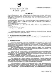
Un elemento <strong>de</strong>finido por tres p<strong>la</strong>nos normales entre sí, está sometido a un estado p<strong>la</strong>no,<br />
cuando <strong>la</strong>s <strong>tensiones</strong> en dos <strong>de</strong> sus caras son nu<strong>la</strong>s.<br />
Analicemos el elemento <strong>de</strong> <strong>la</strong> siguiente figura:<br />
/2010 5
ESTABILIDAD II<br />
CAPITULO III: ELEMENTOS DE LA TEORIA DE TENSIONES Y DEFORMACIONES<br />
dx ds. sen<br />
dy ds. cos<br />
Adoptamos <strong>la</strong>s siguientes convenciones <strong>de</strong> signos:<br />
Tensiones normales: serán positivas cuando produzcan tracción.<br />
Tensiones tangenciales: serán positivas cuando produzcan un giro <strong>de</strong> momento con sentido horario<br />
respecto a un punto interior <strong>de</strong>l prisma.<br />
Angulo : El ángulo se mi<strong>de</strong> a partir <strong>de</strong>l p<strong>la</strong>no vertical y se consi<strong>de</strong>ra positivo cuando es antihorario.<br />
El p<strong>la</strong>no <strong>de</strong>finido mediante el ángulo es paralelo al eje z. Los tres p<strong>la</strong>nos <strong>de</strong>terminados por<br />
los ejes x, y, y el ángulo pasan por el mismo punto; <strong>de</strong> allí que no tenemos en cuenta fuerzas <strong>de</strong> masa<br />
sobre dicho elemento.<br />
Recordamos por Cauchy:<br />
xy yx (3.7)<br />
Tomando en profundidad una distancia unitaria (d z = 1) y p<strong>la</strong>nteando proyecciones <strong>de</strong> fuerzas<br />
sobre <strong>la</strong> dirección 1, por razones <strong>de</strong> equilibrio tenemos:<br />
<br />
<br />
<br />
F s / direc 1 0<br />
ds .1 <br />
<br />
x<br />
dy cos<br />
.1 <br />
xy<br />
dy sen .1 - <br />
y<br />
dx sen .1 <br />
xy<br />
dx cos<br />
.1 0<br />
<br />
<br />
<br />
<br />
<br />
<br />
<br />
<br />
x<br />
<br />
<br />
x<br />
x<br />
x<br />
cos<br />
2<br />
<br />
y<br />
2<br />
sen - 2<br />
xy<br />
sen cos <br />
<br />
2<br />
2 x y x y<br />
cos y<br />
sen - - xy<br />
sen 2 <br />
2 2<br />
<br />
y <br />
<br />
x 2<br />
y 2<br />
(2cos 1) (2sen 1) xy<br />
sen 2 <br />
2 2<br />
2<br />
<br />
y <br />
<br />
x 2<br />
2 y 2<br />
2<br />
(cos sen )<br />
(cos sen )<br />
<br />
xy<br />
sen 2 <br />
2 2<br />
2<br />
<br />
x y x y<br />
<br />
cos 2 sen 2<br />
(3.8)<br />
xy<br />
2 2<br />
/2010 6
ESTABILIDAD II<br />
CAPITULO III: ELEMENTOS DE LA TEORIA DE TENSIONES Y DEFORMACIONES<br />
Simi<strong>la</strong>r a lo anterior, proyectamos fuerzas sobre <strong>la</strong> dirección 2:<br />
<br />
F s / direc 2 0<br />
ds .1 <br />
<br />
x<br />
dy<br />
sen<br />
.1 <br />
xy<br />
dy cos .1 <br />
y<br />
dx cos<br />
.1 <br />
yx<br />
dx sen<br />
.1 0<br />
<br />
<br />
<br />
2<br />
2<br />
<br />
cos<br />
sen cos<br />
sen <br />
x<br />
y<br />
xy<br />
<br />
<br />
<br />
x<br />
<br />
y<br />
<br />
sen2 <br />
xy<br />
cos 2<br />
(3.9)<br />
2<br />
Las <strong>tensiones</strong> vincu<strong>la</strong>das a dos p<strong>la</strong>nos perpendicu<strong>la</strong>res se <strong>de</strong>nominan <strong>tensiones</strong> complementarias.<br />
Para calcu<strong>la</strong>r<strong>la</strong>s po<strong>de</strong>mos reemp<strong>la</strong>zar en <strong>la</strong>s ecuaciones anteriores, que son válidas para cualquier<br />
ángulo , por ( +90º ).<br />
<br />
<br />
<br />
x<br />
y<br />
x<br />
'<br />
<br />
cos 2`<br />
sen2`<br />
xy<br />
2 2<br />
<br />
x y x y<br />
<br />
2<br />
xy<br />
2 2<br />
Si analizamos <strong>la</strong> siguiente suma:<br />
y<br />
<br />
cos 2 <br />
sen <br />
' <br />
x<br />
<br />
y<br />
cte. Invariante <strong>de</strong> <strong>tensiones</strong><br />
(3.10)<br />
po<strong>de</strong>mos ver que <strong>la</strong> suma <strong>de</strong> <strong>la</strong>s <strong>tensiones</strong> normales correspondientes a dos p<strong>la</strong>nos ortogonales se<br />
mantienen constantes, por lo que a esta suma se <strong>la</strong> <strong>de</strong>nomina invariante <strong>de</strong> <strong>tensiones</strong>.<br />
3.4.2 Valores máximos y mínimos<br />
En el ítem anterior hemos visto <strong>la</strong> manera <strong>de</strong> po<strong>de</strong>r calcu<strong>la</strong>r el valor <strong>de</strong> <strong>la</strong>s <strong>tensiones</strong> cuando el<br />
prisma elemental tiene una rotación; ahora vamos a tratar <strong>de</strong> <strong>de</strong>terminar <strong>la</strong> rotación que <strong>de</strong>bería tener<br />
para que <strong>la</strong>s <strong>tensiones</strong> alcancen valores extremos. Para obtener máximos y<br />
mínimos, <strong>de</strong>rivamos e igua<strong>la</strong>mos a cero.<br />
sen2 2<br />
cos 2<br />
0<br />
d <br />
<br />
x y<br />
xy<br />
d<br />
(I<strong>de</strong>m 3.9)<br />
2<br />
xy<br />
tg2 <br />
<br />
(3.11)<br />
<br />
x<br />
y<br />
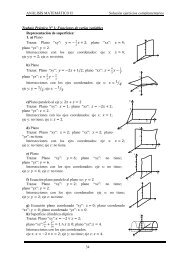
Observando esta última ecuación, po<strong>de</strong>mos ver que <strong>la</strong> misma<br />
queda satisfecha por dos valores <strong>de</strong> , los cuales difieren entre sí 90º. Reemp<strong>la</strong>zando<br />
entonces en <strong>la</strong> ecuación 3.8 por estos valores llegamos a obtener<br />
<strong>la</strong>s expresiones correspondientes a <strong>la</strong>s <strong>tensiones</strong> normales máxima y<br />
mínimas. Para ello nos apoyamos en <strong>la</strong> construcción gráfica <strong>de</strong> <strong>la</strong> figura,<br />
<strong>de</strong> don<strong>de</strong> resulta muy simple obtener los valores <strong>de</strong> cos 2 y sen 2.<br />
/2010 7
ESTABILIDAD II<br />
CAPITULO III: ELEMENTOS DE LA TEORIA DE TENSIONES Y DEFORMACIONES<br />
cos 2<br />
<br />
<br />
<br />
<br />
2 2<br />
<br />
4<br />
<br />
<br />
x<br />
<br />
x<br />
<br />
y<br />
y<br />
xy<br />
sen2<br />
<br />
x<br />
2<br />
y<br />
xy<br />
2<br />
4<br />
xy<br />
2<br />
<br />
<br />
<br />
<br />
x<br />
<br />
2<br />
y<br />
<br />
<br />
<br />
2<br />
x y<br />
x y<br />
xy<br />
xy<br />
2<br />
2<br />
2 2 2<br />
2 2<br />
<br />
4<br />
<br />
4<br />
x<br />
y<br />
xy<br />
x<br />
y<br />
xy<br />
<br />
<br />
<br />
x<br />
<br />
2<br />
y<br />
<br />
2<br />
<br />
<br />
x<br />
<br />
<br />
x<br />
y<br />
<br />
2<br />
<br />
<br />
y<br />
4<br />
2<br />
xy<br />
4<br />
2<br />
xy<br />
2<br />
<br />
max<br />
min<br />
<br />
<br />
x<br />
<br />
2<br />
y<br />
<br />
1<br />
2<br />
2<br />
2<br />
<br />
4<br />
x<br />
y<br />
xy<br />
Si calcu<strong>la</strong>mos el valor <strong>de</strong> para <br />
<br />
x<br />
<br />
y<br />
2<br />
xy<br />
<br />
x<br />
<br />
y<br />
<br />
<br />
<br />
xy<br />
0 (3.12)<br />
2<br />
2 2<br />
2 2<br />
4<br />
4<br />
<br />
x<br />
y<br />
<br />
xy<br />
po<strong>de</strong>mos ver que <strong>la</strong>s <strong>tensiones</strong> máximas y mínimas, no sólo se producen simultáneamente en p<strong>la</strong>nos<br />
ortogonales, sino que al mismo tiempo en dichos p<strong>la</strong>nos <strong>la</strong>s <strong>tensiones</strong> tangenciales son nu<strong>la</strong>s. Las <strong>tensiones</strong><br />
máximas y mínimas se <strong>de</strong>nominan “<strong>tensiones</strong> principales” y los ejes perpendicu<strong>la</strong>res a los p<strong>la</strong>nos<br />
don<strong>de</strong> actúan, “ejes principales”.<br />
A continuación vamos a tratar <strong>de</strong> <strong>de</strong>terminar <strong>la</strong>s <strong>tensiones</strong> tangenciales máximas y mínimas.<br />
<br />
x<br />
<br />
y<br />
<br />
<br />
xy<br />
d<br />
<br />
d<br />
tg2<br />
tg2<br />
<br />
<br />
<br />
<br />
<br />
x<br />
<br />
<br />
<br />
x<br />
y<br />
2<br />
1<br />
<br />
tg2<br />
<br />
<br />
xy<br />
cos 2 2<br />
<br />
y<br />
<br />
xy<br />
2<br />
sen2<br />
0<br />
<br />
difiere<br />
90º<br />
<strong>de</strong><br />
2<br />
<br />
(3.13)<br />
Los p<strong>la</strong>nos don<strong>de</strong> se producen <strong>la</strong>s <strong>tensiones</strong> principales difieren 45º <strong>de</strong> aquellos don<strong>de</strong> <strong>la</strong>s <strong>tensiones</strong><br />
tangenciales son máximas y mínimas.<br />
<br />
max<br />
min<br />
<br />
<br />
<br />
x<br />
<br />
2<br />
y<br />
<br />
<br />
<br />
<br />
<br />
x<br />
<br />
<br />
x<br />
<br />
<br />
y<br />
<br />
2<br />
y<br />
<br />
4<br />
xy<br />
2<br />
<br />
<br />
<br />
<br />
<br />
xy<br />
x<br />
<br />
<br />
2<br />
y<br />
<br />
2<br />
xy<br />
<br />
4<br />
xy<br />
2<br />
<br />
max<br />
min<br />
<br />
<br />
1<br />
2<br />
2<br />
2<br />
<br />
4<br />
(3.14)<br />
x<br />
y<br />
xy<br />
/2010 8
ESTABILIDAD II<br />
CAPITULO III: ELEMENTOS DE LA TEORIA DE TENSIONES Y DEFORMACIONES<br />
Calculemos el valor <strong>de</strong> para , siendo<br />
tg2<br />
<br />
<br />
<br />
x<br />
2<br />
<br />
xy<br />
<br />
<br />
y<br />
<br />
<br />
x<br />
<br />
2<br />
<br />
2<br />
y<br />
<br />
<br />
x<br />
<br />
2<br />
y<br />
<br />
<br />
x<br />
<br />
<br />
2<br />
y<br />
xy<br />
<br />
2<br />
<br />
4<br />
2<br />
xy<br />
<br />
<br />
xy<br />
<br />
x<br />
<br />
y<br />
<br />
x<br />
<br />
<br />
2 2<br />
<br />
4<br />
2<br />
x<br />
y<br />
xy<br />
<br />
y<br />
<br />
x<br />
y<br />
<br />
<br />
(3.15)<br />
3.5 CIRCULO DE MOHR PARA TENSIONES<br />
3.5.1 Trazado y justificación en el estado doble<br />
Si consi<strong>de</strong>ramos <strong>la</strong>s ecuaciones 3.8 y 3.9, y <strong>la</strong>s reor<strong>de</strong>namos, elevamos al cuadrado y sumamos<br />
miembro a miembro tendremos:<br />
<br />
<br />
<br />
<br />
x<br />
<br />
2<br />
y<br />
<br />
<br />
x<br />
<br />
2<br />
y<br />
cos 2 <br />
xy<br />
sen2<br />
<br />
<br />
<br />
<br />
x<br />
<br />
2<br />
y<br />
sen2 <br />
xy<br />
cos 2<br />
2<br />
2<br />
<br />
x<br />
<br />
y <br />
2 <br />
x<br />
<br />
y 2<br />
<br />
<br />
<br />
<br />
<br />
<br />
xy<br />
2<br />
<br />
2<br />
(3.16)<br />
<br />
<br />
<br />
Esta última expresión resulta ser <strong>la</strong> ecuación <strong>de</strong> una circunferencia con centro sobre un eje<br />
asociado a <strong>la</strong>s <strong>tensiones</strong> normales , y <strong>de</strong> abscisa ( x + y )/2 . El radio <strong>de</strong> <strong>la</strong> circunferencia es:<br />
<br />
<br />
<br />
x<br />
<br />
2<br />
y<br />
<br />
<br />
<br />
2<br />
<br />
2<br />
xy<br />
<br />
1<br />
2<br />
2 2<br />
<br />
4<br />
x<br />
y<br />
xy<br />
(3.17)<br />
/2010 9
ESTABILIDAD II<br />
CAPITULO III: ELEMENTOS DE LA TEORIA DE TENSIONES Y DEFORMACIONES<br />
La propiedad fundamental <strong>de</strong> esta circunferencia es que cada punto <strong>de</strong> el<strong>la</strong> está asociado a un<br />
par <strong>de</strong> valores (, ) correspondiente a un p<strong>la</strong>no.<br />
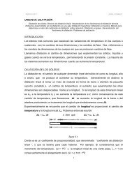
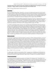
Des<strong>de</strong> el punto <strong>de</strong> vista práctico el trazado<br />
<strong>de</strong> <strong>la</strong> circunferencia es muy simple:<br />
- Ubicamos los puntos A y B <strong>de</strong> coor<strong>de</strong>nadas:<br />
A ( x , xy )<br />
B ( y , yx )<br />
- La circunferencia con centro en C, pasante por<br />
A y B <strong>de</strong>fine el l<strong>la</strong>mado “Circulo <strong>de</strong> Mohr”,<br />
cuyo radio coinci<strong>de</strong> con el indicado en <strong>la</strong><br />
ecuación 3.17<br />
<br />
x<br />
<br />
y<br />
OC <br />
2<br />
<br />
x y<br />
RC <br />
2<br />
(3.18)<br />
r <br />
RC<br />
2<br />
RA<br />
2<br />
<br />
<br />
<br />
<br />
x<br />
<br />
2<br />
y<br />
<br />
<br />
<br />
2<br />
<br />
2<br />
xy<br />
Si por el punto A trazamos una parale<strong>la</strong> a <strong>la</strong> dirección <strong>de</strong>l respectivo y por el punto B trazamos<br />
una parale<strong>la</strong> a <strong>la</strong> dirección <strong>de</strong>l respectivo, dichas rectas se cortan en el punto P, el cual presenta<br />
propieda<strong>de</strong>s muy importantes. Este punto P se <strong>de</strong>nomina “punto principal <strong>de</strong> Mohr”.<br />
Si por el punto principal <strong>de</strong> Mohr trazamos una recta parale<strong>la</strong> al p<strong>la</strong>no respecto <strong>de</strong>l cual <strong>de</strong>seamos<br />
evaluar <strong>la</strong>s <strong>tensiones</strong> actuantes, <strong>la</strong> misma corta a <strong>la</strong> circunferencia en el punto M.<br />
/2010 10
ESTABILIDAD II<br />
CAPITULO III: ELEMENTOS DE LA TEORIA DE TENSIONES Y DEFORMACIONES<br />
A continuación vamos a <strong>de</strong>mostrar que <strong>la</strong>s coor<strong>de</strong>nadas <strong>de</strong> ese punto (OT;MT) se correspon<strong>de</strong>n<br />
con los valores <strong>de</strong> y .<br />
Para ello, previamente justificaremos <strong>la</strong>s siguientes re<strong>la</strong>ciones trigonométricas entre ángulos<br />
presentes en <strong>la</strong> Fig. 3.8, que utilizaremos para <strong>la</strong> referida <strong>de</strong>mostración.<br />
a) / 2<br />
en <br />
DAE :<br />
DA 2. r . cos <br />
en<br />
<br />
<br />
DAA':<br />
AA' DA .sen 2.<br />
r . cos<br />
.sen<br />
<br />
<br />
r .sen 2 <br />
a<strong>de</strong>mas:<br />
<br />
<br />
en CAA':<br />
AA' <br />
r .sen <br />
entonces: / 2<br />
b) 2 . <br />
<br />
en PAC :<br />
<br />
<br />
al<br />
ángulo APC lo <strong>de</strong>nominamos<br />
tenemos <br />
<br />
<br />
PAC será : 2 <br />
( )<br />
<br />
luego<br />
2 4 2 <br />
180º<br />
<br />
<br />
en PCM<br />
2 2 2 <br />
180º<br />
restando m.a.m.<br />
2 - 0<br />
<br />
2 <br />
Una vez <strong>de</strong>mostradas ambas re<strong>la</strong>ciones, <strong>de</strong>finimos el ángulo <br />
2 <br />
OT<br />
OC CT<br />
OC r<br />
cos OC r<br />
<br />
cos 2 <br />
<br />
OT<br />
OC r(cos 2<br />
cos sen2<br />
sen)<br />
<br />
<br />
x<br />
<br />
2<br />
y<br />
r<br />
cos 2<br />
<br />
x<br />
<br />
2r<br />
y<br />
r<br />
sen2<br />
<br />
xy<br />
r<br />
OT<br />
<br />
<br />
x<br />
<br />
2<br />
y<br />
<br />
<br />
x<br />
<br />
2<br />
y<br />
cos 2<br />
<br />
xy<br />
sen2<br />
<br />
<br />
Ec.(3.8)<br />
/2010 11
ESTABILIDAD II<br />
CAPITULO III: ELEMENTOS DE LA TEORIA DE TENSIONES Y DEFORMACIONES<br />
TM<br />
rsen<br />
rsen 2 <br />
<br />
<br />
rsen2<br />
cos r cos 2<br />
sen<br />
TM<br />
<br />
<br />
x<br />
<br />
2<br />
y<br />
sen2 <br />
xy<br />
cos 2<br />
<br />
<br />
Ec.(3.9)<br />
El círculo <strong>de</strong> Mohr no sólo resulta práctico para <strong>de</strong>terminar <strong>la</strong>s <strong>tensiones</strong> presentes en un p<strong>la</strong>no<br />
cualquiera, sino que a partir <strong>de</strong>l mismo pue<strong>de</strong>n obtenerse <strong>la</strong>s <strong>tensiones</strong> principales y sus p<strong>la</strong>nos principales,<br />
o <strong>la</strong>s <strong>tensiones</strong> tangenciales máxima y mínima. En el círculo <strong>de</strong> <strong>la</strong> figura 3.9 hemos representado<br />
<strong>la</strong>s <strong>tensiones</strong> recientemente mencionadas y sus correspondientes p<strong>la</strong>nos <strong>de</strong> actuación. En el mismo<br />
también pue<strong>de</strong> verse que en correspon<strong>de</strong>ncia con <strong>la</strong>s <strong>tensiones</strong> principales existen tangenciales<br />
nu<strong>la</strong>s.<br />
a) Corte puro<br />
A través <strong>de</strong>l círculo <strong>de</strong> Mohr po<strong>de</strong>mos analizar algunos casos particu<strong>la</strong>res que nos interesan.<br />
/2010 12
ESTABILIDAD II<br />
CAPITULO III: ELEMENTOS DE LA TEORIA DE TENSIONES Y DEFORMACIONES<br />
En este estado vemos que existe un elemento girado a 45º con respecto al solicitado por corte<br />
puro, tal que sus caras están sometidas a <strong>tensiones</strong> normales <strong>de</strong> tracción y compresión, iguales en valor<br />
absoluto y numéricamente iguales a <strong>la</strong> tensión tangencial.<br />
b) Tracción simple<br />
3.5.2 Trazado en el estado triple<br />
Así como es posible <strong>de</strong>terminar <strong>la</strong>s <strong>tensiones</strong><br />
principales en un estado doble, éstas también pue<strong>de</strong>n<br />
calcu<strong>la</strong>rse en un estado triple. Si suponemos que estas<br />
<strong>tensiones</strong> son conocidas, es posible <strong>de</strong>mostrar que el<br />
par <strong>de</strong> <strong>tensiones</strong> (,) correspondiente a un p<strong>la</strong>no inclinado<br />
cual-quiera se correspon<strong>de</strong> con <strong>la</strong>s coor<strong>de</strong>nadas <strong>de</strong><br />
cierto punto ubicado <strong>de</strong>ntro <strong>de</strong>l área rayada indicada en<br />
<strong>la</strong> figura 3.12, encerrada por los círculos, <strong>de</strong>finidos, en<br />
este caso por <strong>la</strong>s tres <strong>tensiones</strong> principales.<br />
Un hecho importante a <strong>de</strong>stacar es el que<br />
se observa en el círculo <strong>de</strong> <strong>la</strong> fig. 3.13. Allí tenemos<br />
un estado triple don<strong>de</strong> 3 =0, y pue<strong>de</strong><br />
verse que <strong>la</strong> tensión tangencial máxima resulta<br />
mayor que <strong>la</strong> que correspon<strong>de</strong>ría al estado p<strong>la</strong>no<br />
corre<strong>la</strong>cionado con <strong>la</strong>s <strong>tensiones</strong> principales 1<br />
y 2 exclusivamente.<br />
/2010 13