Teoria di campo medio per l'antiferromagnete di Ising

Teoria di campo medio per l’antiferromagnete di
Ising
L. P.
24 Novembre 2005
Consideriamo la hamiltoniana di Ising, definita su un reticolo cubico semplice
in d dimensioni, con coefficiente di interazione −J, dove J > 0:
H(σ) =
Jσiσj −
hσi. (1)
È ragionevole aspettarsi, in questa situazione, che gli stati di più bassa energia
corrispondano a configurazioni in cui spin primi vicini puntano prevalentemente
in direzioni opposte. Per descrivere questa situazione, suddividiamo il reticolo
in due sottoreticoli: il sottoreticolo pari, in cui la somma delle coordinate
(espresse in unità del passo del reticolo) è pari, e il sottoreticolo dispari. Se
i appartiene, per esempio, al sottoreticolo pari, ciascuno dei suoi primi vicini
apparterrà al sottoreticolo dispari. Definiamo quindi la magnetizzazione
alternata N mediante l’espressione
N =
ǫiσi, (2)
i
dove ǫi = +1 se i appartiene al sottoreticolo pari, e ǫi = −1 se appartiene al sottoreticolo
dispari. D’altra parte, possiamo anche considerare la magnetizzazione
M, definita come al solito da
M =
σi. (3)
Indichiamo con m ed n la magnetizzazione e la magnetizzazione alternata per
spin:
m = M N
, n = , (4)
N N
dove N è il numero totale di spin.
Desideriamo studiare il sistema in approssimazione di campo medio. Ci
aspetteremo che il valor medio dello spin 〈σi〉 abbia valori diversi nei due
sottoreticoli. Indichiamo con m+ (rispettivamente m−) questo valore per il
sottoreticolo pari (rispettivamente dispari). Si ha ovviamente
m = m+ + m−
2
i
i
; n = m+ − m−
. (5)
2
1

Quindi
m+ = m + n; m− = m − n. (6)
Possiamo adesso valutare l’entropia S0 che compare nell’espressione dell’energia
libera di prova nella teoria di campo medio. Avremo N/2 spin con magnetizzazione
m+ e altrettanti con magnetizzazione m−. L’entropia per spin di un
paramagnete con magnetizzazione x è data da
Quindi
s(x) = −kB
1 + x
2
log
1 + x
2
+
1 − x
2
log
1 − x
2
. (7)
S0 = N
2 [s(m+) + s(m−)] = N
[s(m + n) + s(m − n)] .
2
(8)
L’energia libera di prova, espressa in funzione di m ed n, è quindi data da
F(m,n) = N − ζJn2
T
− hm − [s(m + n) + s(m − n)] ,
2 2
(9)
dove ζ = 2d è il numero di coordinazione del reticolo. Ricordando che
ds
dx = −kB tanh −1 x, (10)
possiamo ottenere le equazioni di autoconsistenza per m ed n:
h = kBT
2
ζJn = kBT
2
tanh −1 (m + n) + tanh −1 (m − n) ; (11)
tanh −1 (m + n) − tanh −1 (m − n) . (12)
Evidentemente queste equazioni ammettono sempre la soluzione banale con n =
0 e con
h
m = tanh .
kBT
(13)
Vediamo in quali condizioni è possibile ottenere delle soluzioni stabili con n = 0.
Poiché
tanh(m + n) = tanh(m) +
otteniamo
n mn2
+
1 − m2 (1 − m2 ) 2 + (1 + m2 ) 2n3 3(1 − m2 ) 3 + o(n3 ), (14)
1 −1 −1 n
tanh (m + n) − tanh (m − n) =
2
1 − m2 + (1 + m2 ) 2n3 3(1 − m2 ) 3 + o(n3 ). (15)
Quindi, per piccoli valori di n, otteniamo l’equazione
ζJ
kBT −
1
1 − m 2
n ≃ (1 + m2 ) 2n3 3(1 − m2 . (16)
) 3
2

Questa equazione ammette soluzioni con n reale solo se il fattore fra parentesi
a primo membro è positivo. Abbiamo quindi identificato la linea di transizione
Tc(m) in funzione della magnetizzazione per spin m:
kBTc(m) = (1 − m 2 )ζJ. (17)
Vediamo che, per m = 0, la temperatura critica è uguale a quella del modello
di Ising ferromagnetico. Però, all’aumentare di |m|, la temperatura tende a
0. È anche interessante considerare la linea di transizione Tc(h) in funzione
del campo magnetico applicato h. Poiché m, h e T sono collegati dalla (13),
dobbiamo risolvere la seguente equazione in Tc:
kBTc = 1 − tanh 2 (h/kBTc) ζJ. (18)
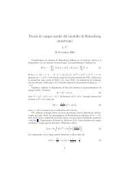
In realtà è molto più semplice esprimere parametricamente Tc(m) tramite la
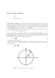
(17) e h(Tc,m) invertendo la (13). Si ottiene così il diagramma di fase mostrato
in figura 1, in cui gli stati con n = 0 sono all’interno della curva, e le temperature
sono misurate in unità Tc(0). Notiamo che, se h = 0, c’è una regione in cui si ha
1
0.8
0.6
0.4
0.2
T
-0.4 -0.2 0.2 0.4
Figura 1: Diagramma di fase per l’antiferromagnete di Ising nel piano (h,T).
La fase antiferromagnetica è all’interno della curva.
un comportamento rientrante della fase antiferromagnetica: si passa dalla fase
disordinata alla fase antiferromagnetica abbassando la temperatura al disotto di
una temperatura Tc1; poi però, a una temperatura Tc2 < Tc1, il sistema ritorna
nella fase disordinata.
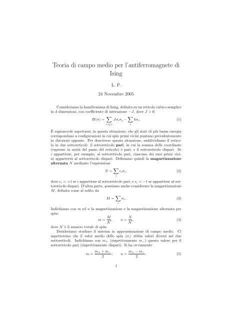
Notiamo che l’andamento della suscettività χ = ∂m/∂h cambia quando n
diventa non nullo. per piccoli valori di |n|, abbiamo infatti dalla (11), tenendo
conto della (14),
h ≃ kBT
tanh(m) + mn2
(1 − m2 ) 2
. (19)
3
h

χ
1
0.8
0.6
0.4
0.2
0.5 1 1.5 2
Figura 2: Suscettività magnetica χ = ∂m/∂h in funzione di T, lungo la linea
h = 0. La temperatura è misurata in unità di Tc.
Il secondo termine di questa equazione è proporzionale a m[Tc(m) − T] (con un
coefficiente positivo). Quindi la derivata di χ rispetto a T subisce una discontinuità
per T = Tc. Per esempio, in figura 2 viene mostrata la suscettività in
funzione di T lungo la linea h = 0. In questo caso, è facile vedere che
χ =
1 − n2
. (20)
kBT
4
T