Dynamics and motion control - KTH

Dynamics and motion control 

KTH MMK 

Date: 2011-01-14 

File: Q:\md.kth.se\md\mmk\gru\mda\mf2007\arbete\Lectures\FinalVersions\For2011\L1.fm 

Lecture 1 

Course introduction and overview 

Date: 2011-01-14 


Bengt Eriksson, Jan Wikander 

KTH, Department of Machine Design 

Division of Mechatronics 

e-mail: {benke, jan}@md.kth.se 

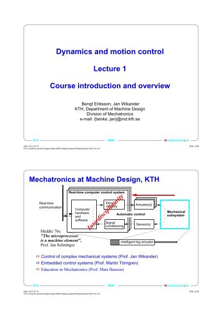
Mechatronics at Machine Design, KTH 

Real-time 

communication 

Computer 

hardware 

and 

software 

Middle 70s: 

"The microprocessor 

is a machine element", 

Prof. Jan Schnittger 

Real-time computer control system 

Drive 

circuitry 

� Control of complex mechanical systems (Prof. Jan Wikander) 

� Embedded control systems (Prof. Martin Törngren) 

� Education in Mechatronics (Prof. Mats Hanson) 


Signal 

conditioning 

Interdisciplinarity 

Actuator(s) 

Actuator(s) 

Automatic control 

Sensor(s) 

. intelligent leg actuator 

Mechatronics Lab 

Mechanical 

subsystem 


Slide: 1(35) 

Slide: 2(35)

Motivation: multidisciplinarity is required! 

Mechanics 

development 

CAD 

Dynamics 

FEM 


Date: 2011-01-14 


1.1. Lecture outline 

• 1. Course goal 

Analysis and specifications 

Conceptual design, functions, technical implementation 

Control function Software- Electronics 

development development development 

Integration 

• 2. Course implementation 


Date: 2011-01-14 


Application 

software 

Supporting software 

Input/output drivers 

Hardware 

Network 


• 3. Overview of and introduction to modelling and control of 

mechanical systems 


Slide: 3(35) 

Slide: 4(35)

1.1.1 Overall course goal 

To provide an understanding and the skills of modelling and 

design of motion control systems; 

"from modelling to implementation" 


Date: 2011-01-14 


1.1.2 After the course you should be able to 

• Specify overall performance requirements for a motion control system 

• Derive models of typical mechatronic applications 


Date: 2011-01-14 



• Find good parameters of dynamic models in both frequency and time domain 

• Design model based feedback and feed forward control both in continuous and 

discrete time 

• Simulate process and control system models in both continuous and discrete time 

• Design and structure the controller software for microprocessor implementation 

• Understand the limitations and restrictions due to computing speed. 

Read more in the course PM 


Slide: 5(35) 

Slide: 6(35)

1.1.3 Further course goals 


Date: 2011-01-14 




Date: 2011-01-14 


Learning how your theoretical knowledge from earlier 

courses in math, mechanics, 

numeric methods and control should best be 

used to avoid chaos in real world experiments. 




• 3. Overview of and introduction to modelling and control of 

mechanical systems 


Slide: 7(35) 

Slide: 8(35)

1.2.1 Prerequisites 

• Some mechanical and electrotechnical knowledge 

• Very litle programming knowledge 

• Good control knowledge it should corespond to the content of a basic 

course in control engineering 


Date: 2011-01-14 


1.2.2 Course outline 

• 2 two hour lectures per week (except first week -> three) 

• Basic theory and calculated examples 

• 2 three hour per week lab working 

• Mainly computer simulation work, Matlab/Simulink 

• Woking with Exercises and Workshops 

• Assistance by 

Suleman Khan 

Ashan Qamar 


Date: 2011-01-14 




Slide: 9(35) 

Slide: 10(35)

1.2.3 Literature and course material 

� The course specification 

� The reading material 

� The lecture notes 

�Standard book in control 

� The exercises 

� The workshops 


Date: 2011-01-14 


1.2.4 Examination 

• 1. Completed exercises 


Date: 2011-01-14 


L2, modelling 

L3, feedback design in continuous time 

L4, feedback design in discrete time 

L5, Model following control -servo 

L6, Implementation on real-time HW 

L7, Robustness issues 


• The exercises are completed by showing the results to an assistant in the lab. 

Exercises part 1, modeling of mechanical systems 

Exercises part 2, modeling of a DC motor system 

Exercises part 3, control of a DC motor system 

• 2. Written reports on the workshops, A and B. 

• 3. Written exam. 

Grading: A-F according to ECTS based on a weighted combination of the 

bullets 2 and 3 above. 


Slide: 11(35) 

Slide: 12(35)

1.2.5 Exercises and laboratory facilities 

• Working in groups of preferably three people in each group 

• Where to work? 

- MMT computer rooms: Matlab/Simulink 

- Mechatronics-lab: ("FIM-labbet") Matlab/Simulink and experiments on real 

motor. 

- Wennström-lab: ("elektro-labbet") Matlab/Simulink 

- Your own computers, KTH CD’n with Matlab/Simulink 

• Mechatronics-lab: "passerkort": need card numbers 

• The labs are free to use 7/24 if they not are booked for other courses, booking 

schedule is available from course home page. 

• The course material and course web: www.md.kth.se/mmk/gru/mda/MF2007/ 


Date: 2011-01-14 


1.2.6 Additional useful material 

• The course builds upon earlier courses! 

- math, mechanics, machine elements, numerical methods, control 

engineering, 

computer science and programming, electrical engineering 

• General textbooks in 


Date: 2011-01-14 



• Control engineering -from a first course in automatic control. e.g. Glad och Ljung: 

Reglerteknik - Grundläggande teori 

• Electric circuit theory -from a first course in electric circuits. e.g. Hans Johansson 

Elektroteknik 

• Mechanical enginering. -from a course in dynamics. e.g. ------ 


Slide: 13(35) 

Slide: 14(35)

1.2.7 File system, AFS 

• Disk space for each person is given by kth.se 

Path: \afs\kth.se\home\"first letter in account"\"second letter in account"\"account 

name"\ 

• Log in with Kerbrose using your kth.se account and password. 

• Map your home account path to the computer using AFS Client 

(could have changed from last year) 

• The main advantage is that you can work with your own applications 

on any computer where Kerbrose and the AFS client are installed as if 

they were on the local disc. No need for copying files. 


Date: 2011-01-14 


1.2.8 Learning philosophy 

• It is about your learning - for which You is the boss! 

Date: 2011-01-14 



• We employ feed forward and feedback to improve the learning process 

• Feed forward concepts: material, lectures, the project etc. 

• Feedback mechanisms 

1) Participant representatives: to collect important feedback info 

2) Lecture and workshop follow up questions 

3) Hand ins of project parts 

4) Course evaluation in the end 



Slide: 15(35) 

Slide: 16(35)




• 3. Overview of and introduction to control of mechanical 

systems 

and a brief introduction to tools 


Date: 2011-01-14 


1.3.1 Forecasts! 


Date: 2011-01-14 



• "I think there is a world market for about five computers", Tomas J Watson Sr, 

IBM 1943 

• "There are no reasons for any individuals to have a computer in their home", 

Ken Olson, Digital Equipment 1977 

• "The current rate of progress cannot continue much longer", various computer 

technologists, 1950 

’Moore’s law’ (Intel, 1965): 

Microelectronics (MOS) performance is ~doubled every 18 months and chip 

size is reduced by 50% 

Intel 4004/1971 vs. Intel Pentium/1996: from 2300 to 5.5 million transistors 

One prediction for "2006: One chip with 200M transistors with 2GHZ frequency" 


Slide: 17(35) 

Slide: 18(35)

1.3.2 Control technologies over time 

Mechanical, hydraulic and 

pneumatic controllers 

(e.g. centrifugal regulator, 

18th century) 


Date: 2011-01-14 


Combustion engine 

19th century 

(Pneumatic controllers 

early 20th century) 

Electrical relays 

(Babbages analytical 

Analogue electronic controllers 

(1940-50) 

engine, ~1840) (transistor, 1947) 

Direct digital 

control 

(early 1960:ies) 

Distributed 

computer control 

(~1970:ies) 

(4004 microprocessor, 1971) 

1.3.3 Control development over time 

Date: 2011-01-14 



• All mechanical controllers, e.g. the centrifugal governor (wind mills, steam engines, 

telephones), from 1700 and onwards. 

• Early theoretical results, e.g Routh, Hurwitz and Lyapunov on stability, late 1800’s. 

• Ziegler’s and Nichols’ method for tuning of PID controllers in 1942. 

• Computers in control from the mid 50’s. 

• New control design methods in the late 20th century: Optimal, Adaptive, Non-linear, 

Robust, Fuzzy, Neural, etc. 

• Still in use! 

- Mechanical controllers, e.g the flapper servo stage in hydraulic valves. Temperature 

control in shower taps. 

- Analog electronic controllers, e.g. for PID control 



Slide: 19(35) 

Slide: 20(35)

1.3.4 The paradigm shift 

Servo steering with 

mechanical backup 


Date: 2011-01-14 


Date: 2011-01-14 


Steer by wire 

1.3.5 What can be achieved? 

Hy-Wire from GM 

(autonomy 2) 


� More digital control! 



Slide: 21(35) 

Skateboard concept 

Fuel cell 94kW 

Integrated distributed control 

Weight: 2 tons, Distance: 480km 

Slide: 22(35)

1.3.6 Why models? - active body control 

• Many sensors 

• 4 actuators 

• Complex dynamics 

• Mechanical and 

control design not 

separable 

• Simulation necessary 

sensors 

actuators 


Date: 2011-01-14 


1.3.7 More than just feedback 

Trajectory 

planner 

Implemented on embedded 

control platform 

Mode logic 

Diagnostics 

Model following 


References 

Human machine 

interface 

Feedback 



Date: 2011-01-14 


Observer 

Actuator 

Disturbance 

Controlled process 



Slide: 23(35) 

Output 

Sensors 

Slide: 24(35)

1.3.8 Example motion control applications 

• Industrial robot control 

• Vehicular systems (suspension, brakes, engine control...) 

• Aircraft control and space applications 

• Axis control in various production machines 

• Hydraulic servo, e.g. in forest harvester or excavator 

• Master and slave control in teleoperated systems 

• Mobile robots/machines 


Date: 2011-01-14 


1.3.9 The complete control design process 

• Design of the mechanical system 

Either prior to, or in conjunction with control design 

Date: 2011-01-14 



• Modelling of the system and in some cases also modelling of the system’s 

interaction with the environment 

• Analysis of dynamic properties including simulation 

• Control requirement specifications 

• Control design including choice of related components such as sensors, 

control computer and sometimes actuator(s) 

• Simulation, verification and control prototyping 

• Real-time implementation 



Slide: 25(35) 

Slide: 26(35)

1.3.10 Mechanical system modelling 

• Degrees of freedom - DOF: The number of inertia in a dynamic system 

that can move relative each other 

• The motion of each DOF is modelled by, , or = . 

Example: 

m 1 

k d y 2 


Date: 2011-01-14 


F 

m 2 

∑ 

mx ·· = Fy Jϕ ·· 

1.3.11 Modelling and dynamic analysis 

of mechanical systems 

• Putting up the differential equations 

• Linearization 

y 1 

• Formulations: 

- State space; matrix equations 

- Input-output; transfer functions 


Date: 2011-01-14 


∑ 

M y 

Two DOFs coupled by a weak link. 

4:th order differential equation 


• Different levels of simplification depending on purpose, e.g. simulation vs 

control design, feed forward vs feedback - model validation 

• Finding the parameters; system identification 

• Computer tools such as Maple and Matlab e.g. with the Identification toolbox 


Slide: 27(35) 

Slide: 28(35)

.6 

.4 

.2 

1 

.8 

.6 

.4 

.2 

1.3.12 Different domains for different tasks 

yt () A 

i 

e λ – it = cos( 

ω 

i 

t + φ 

i 

) 

∑ 

0 

0 5 10 15 20 25 30 

Time 

domain 

10 −1 

−40 


Date: 2011-01-14 


1.3.13 Feedback control 

Date: 2011-01-14 


Gain dB 

Phase deg 

20 

0 

−20 

0 

−90 

−180 

10 −1 

Gs ( ) 

Different controller structures 

• PID control: 

= 

10 0 

Frequency (rad/sec) 

10 0 

Frequency (rad/sec) 


dx 

----- = fxu ( , ) y = h( x) 

dt 

2 

ω0 s 2 

---------------------------------------- 

2 

+ 2ξω0 s + ω0 t 

d 

ut () = Kp ⋅ et () + KI ⋅ ∫es 

( ) ds+ 

KD⋅ et () 

dt 

0 

10 1 

10 1 

Frequency domain 

+ 

+ 

Im 

Complex plane 

Re 


• Cascade control: inner loop viewed as an ideal servo by outer loop 

y ref 

Controller 2 

z ref 

Controller 1 

u 

G 1(s), e.g. 

actuator 

z 

Controlled 

system, G 2(s) 

y 


Slide: 29(35) 

Slide: 30(35)

1.3.14 Feedback control properties 

The main principle in control engineering 

• Typically model based (but not required to be) 

• Produces control signals after an error has occurred 

• Disturbance rejection is achieved 

• Effect of process parameter variations is reduced 

• Leads to a closed loop 

• Sensor noise may be amplified and deteriorate performance 

• May lead to instability if designed incorrectly 


Date: 2011-01-14 


1.3.15 Discrete time control 

Digital control system 

Constant sampling frequency 


Date: 2011-01-14 



y(tk) u(tk) u(t) 

Sampling Controller 

Actuation 

Continuous time y(t) 

process 

Synchronized actions 

Sampling interval h = t k - t k-1 

Sampling frequency f = 1/h 

Other tasks 

Antialiasing filter 

y, y(t k) 

e.g. communication and 

diagnostics 

h 

Sensor 


t 

Slide: 31(35) 

Slide: 32(35)

1.3.16 Brief introduction to tools 

• Modelling and simulation 

+ Matlab/Simulink 

+ Purpose: Modeling, analysis and design + model verification 

• Rapid control prototyping (RCP), 2 different systems 

dSPACE 


Date: 2011-01-14 


Date: 2011-01-14 


- Power PC on PCI bus inside PC 

- I/O on the same PCI board 

- Programmed with Simulink 

- RTW, C-code generator 

- Microtec C cross compiler 

- 4 systems in lab 

- Host PC env. ControlDesk 

1.3.17 Modelling and simulation 

u Simulated 

process 

y 

Real process 

abstraction 


dx 

----- = fxu ( , ) y = h( x) 

dt 


• Numerical solution: non real-time 


Slide: 33(35) 

Integration solvers, e.g., runge kutta order 

2-5 using variable step size for 

efficient simulation time and 

stable solution. 

Slide: 34(35)

1.3.18 Rapid control prototyping (RCP) 

Non real-time 

simulation 

Include I/O 

drivers 

Automatic 

C-code 

generation 


Date: 2011-01-14 


Modelling 

and design 

Control implementation 

needs tools for 

quick iterations 

Evaluate and 

redesign 

Instrumentation 

for tuning and 

measurement 

Compile and 

down load 

on RCP HW 


Slide: 35(35)

Dynamics and motion control - KTH

You also want an ePaper? Increase the reach of your titles

Delete template?

Save as template?