Statistical Inference After an Adaptive Group Sequential Design: A ...

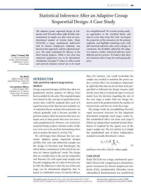
Lothar T. Tremmel, PhD 

Sr. Director and Group 

Leader, Clinical Oncology, 

Cephalon Inc, Frazer, 

Pennsylvania 

Key Words 

Adaptive design; Group 

sequential design; Statistical 

inference 

Correspondence Address 

Lothar Tremmel, PhD, 

Cephalon, Inc, 41 Moores 

Road, Frazer, PA (email: 

Lothar@tremmel.net). 

Drug Information Journal, Vol. 44, pp. 589–598, 2010 • 0092-8615/2010 

Printed in the USA. All rights reserved. Copyright © 2010 Drug Information Association, Inc. 

b i o s t a t i s t i c s 589 

Statistical Inference After an Adaptive Group 

Sequential Design: A Case Study 

The adaptive group sequential design of Lehmacher 

and Wassmer allows fully flexible redetermination 

of sample size after each of a predetermined 

number of interim looks. Study 

02CLLIII, a large, randomized, multicenter 

trial in chronic lymphocytic leukemia, was 

based on this approach, with five planned analyses. 

The study terminated for efficacy at the 

third interim analysis. While it was clear how 

statistical significance was to be determined, 

calculations of proper P values as well as point 

and interval estimates turned out to be much 

i N t R o D U c t i o N 

THE ADAPTIVE GROUP SEQUENTIAL 

DESIGN 

Group sequential designs (GSDs) that allow for 

preplanned interim analyses of efficacy have 

been available for decades. The original designs 

were based on the concept of equal data increments: 

data could be analyzed after each of k 

equal fractions of the data became available (1). 

As statistical theory evolved, this restriction was 

relaxed gradually, and it became possible to 

perform analyses after increments that were unequal, 

even at time points that were not necessarily 

preplanned (2). However, one restriction 

remained firmly in place: interim results of efficacy 

were not to be used for determining when 

next to analyze the data (3, section 7.4). 

We call designs that eliminate this last constraint 

adaptive group sequential designs 

(aGSD). One early and influential example was 

the design of Proschan and Hunsberger (4), 

which allows continuation of the trial if one obtains 

an “almost significant” result. The design 

that we consider here is the one by Lehmacher 

and Wassmer (5), with equal stage weights and 

Pocock’s stopping rule: it is akin to Pocock’s early 

GSD; the difference is that the size of the next 

stage can be determined adaptively, that is, 

based on unblinded review of interim efficacy 

less straightforward. We extend existing analysis 

approaches to the stratified binary and 

time-to-event data from this trial, investigate 

the properties of the estimators for the primary 

endpoint, and highlight remaining issues with 

full statistical inference after such a design. In 

conclusion, the flexibility offered by the adaptive 

features renders statistical inference more 

difficult and less precise. We believe that there 

are situations where it may be worth paying this 

price. 

data. For instance, one could recalculate the 

sample size needed to maintain the power under 

a certain effect size assumption. Importantly, 

rigid rules like that one do not have to be prespecified 

or followed; the design remains valid 

(in the sense that it controls the type I error) no 

matter how the decision regarding the size of 

the next stage is made. Only two design elements 

need to be predetermined: the number of 

interim looks, and the size of the first stage. 

The design works by reestablishing Pocock’s 

equal increment structure for the adaptively 

determined unequally sized stages: under H 0 , 

the standardized effect size from each stage k 

follows an independent standard normal distribution 

if weighted by the square root of the 

stage’s sample size. The test statistic S K is simply 

the standardized sum of these independent, 

standard-normally distributed z values, 

∑ 

S = 1 K Z 

K k 

k = 1.. K 

and hence Pocock’s critical z values apply. 

(1) 

CASE STUDY 

Study 02CLLIII was a large, randomized, openlabel 

clinical trial, comparing two chemotherapeutic 

treatments for chronic lymphocytic leukemia 

(CLL): bendamustine (Treanda) versus 

chlorambucil. Randomization was stratified by 

Submitted for publication; July 2, 2009 

Accepted for publication: December 9, 2009

590 b i o s t a t i s t i c s 

Tremmel 

Binet stage (B vs C) which was believed to be an 

important predictor. Efficacy was measured by 

two key endpoints: tumor response and progression-free 

survival (PFS). The primary endpoint, 

tumor response, was defined as an outcome 

of partial response or better, based on 

predetermined assessment criteria. The key secondary 

endpoint, PFS, was the time from randomization 

to progression of the disease, or 

death from any cause. A sequential testing strategy, 

based on testing response rate first, was 

used to protect the overall type I error. 

An aGSD following Lehmacher and Wassmer 

(5) with equal weighting of the study stages was 

planned in the protocol. Four interim and one 

final analysis were planned, and the first analysis 

was to be done after 80 patients were enrolled. 

Pocock’s method was chosen for determining 

the critical boundaries, yielding equal critical P 

values of 0.016 at each of the five analysis time 

points, corresponding to a planned overall twotailed 

alpha of 5%. A data monitoring committee 

(DMC) was established to assess the interim 

results and to determine, at each interim analysis, 

whether the study should continue. No formal 

futility rules were planned or implemented. 

The protocol also discussed the sample sizes 

that would be needed for a fixed-sample trial: 

n = 84 (total) for tumor response, and n = 326 

(total) for PFS. This was based on effect sizes of 

30% versus 60% response, and a hazard ratio of 

1.429, respectively. The first result was used to 

determine the size of the first study stage (first 

interim analysis to be done after 80 patients), 

and the second result formed the basis of a projected 

maximum sample size of n = 350. 

The study stopped for efficacy at the third interim 

analysis. Unadjusted P values from the 

first three analyses are shown in Table 1. The P 

values are based on statistic Eq. 1 but they are 

not adjusted for the interim analyses. 

Design and results of the study are published 

(6); we note that the results described in this 

article are different because they are based on 

an algorithmic determination of tumor response 

that was used to inform the US product 

label whereas the results in Knauf et al. are 

based on assessments of an independent clini- 

cal data review committee. Moreover, the analysis 

in Knauf et al. incorporates some more data 

points that became available after the third interim 

analysis. 

ISSUES WITH STATISTICAL INFERENCE 

Statistical Significance. Since the nominal 

two-sided P values at the third analysis are lower 

than 0.016, significance at the two-sided level of 

significance of 5% can be claimed. 

Adjusted P Value. Rather than only reporting 

whether the result is significant, it is desirable 

to report the P value as well, to indicate the 

strength of evidence (7). In traditional GSDs, 

correctly adjusted P values can be readily calculated 

with standard software once one agrees on 

how to order the sample space (8). In our aGSD, 

there is no clearly defined sample space to begin 

with as no rigid rules for calculating the 

next stage size are required. Hence, the algorithms 

from GSDs cannot be applied. 

Point Estimate. It would also be desirable to report 

a point estimate for the effect size. Simple 

estimates that ignore the group sequential nature 

of the data—so-called naive estimates— 

are biased; this has been known since the early 

days of such designs (9). Various methods for 

bias adjustments exist (10) and have been implemented 

in standard software for traditional 

GSDs. As Coburger and Wassmer (11) point out, 

the aGSD contributes an additional complication: 

the naive estimator is not a function of the 

test statistic S K , and therefore it is not consistent 

with it: Cases can be constructed where S K would 

indicate maximum support for H 0 whereas the 

naive estimator would yield a value different 

from zero. This will not be the case for an estimator 

that is f(S K ), that is, a function of S K . Another 

advantage of f(S K ) is that under certain assumptions, 

the density of S K is known, and 

therefore the density of f(S K ) will also be known, 

rendering it possible, in principle, to calculate 

its bias. 

Confidence Interval (CI). Finally, confidence 

intervals are needed for complete statistical in-

Inference After Adaptive GSD b i o s t a t i s t i c s 591 

ference. For traditional GSDs, “tight” CIs can be 

developed (3, chapter 8); these require a rigidly 

defined sample space for which the densities 

can be calculated for different alternative hypotheses. 

In the aGSD, the sample space is less 

rigidly defined, and therefore these methods 

cannot be used. 

M E t H o D s 

ADjUSTED P VALUE 

The statistical analysis plan (SAP) had suggested 

calculating the P value based on stagewise 

ordering of the sample space (3, section 8.4). 

Upon data monitoring board (DMB) recommendations, 

the trial continued despite early 

crossing of the efficacy boundary, which is not 

consistent with the proposed method as it assumes 

strict adherence to stopping rules. 

Wright’s (12) concept of a P value does not require 

ordering an ill-defined sample space. The 

P value is understood as the answer to the question: 

What is the smallest level of significance 

α′ for which the given result would have been 

significant? It can be shown that the answer to 

this question is indeed a P value (appendix 1). 

Wassmer (13) proposes the same approach 

specifically for the aGSD and calls it “overall P 

value.” 

In our study, the unadjusted P values were 


Tremmel 

two response rates. As z k , we used the unsquared 

version of the familiar Mantel- 

Haenszel statistic Q MH , with Binet stage as the 

stratification factor. It can be shown (appendix 

2) that this z k can be decomposed into w k *ϑ ˆ , 

where ϑ ˆ is a weighted average of the observed 

within-stratum probability differences, and 

the weights are functions of the margins of the 

2 × 2 tables involved. 

STRATIFIED TImE-TO-EVENT DATA 

The independence of the k increments in the 

log-rank statistic has been established by Tsiatis 

(16), and Wassmer (13) showed that this applies 

to the aGSD as well. Jahn-Eimermacher et al. 

(17) showed how data arising from an aGSD can 

be decomposed correctly into these independent 

increments, each of which can be analyzed 

by an unsquared log-rank test, yielding z k . In our 

case, z k is the kth increment of the familiar logrank 

statistic, with Binet stage as the stratification 

factor. It can be shown that this z k can be 

decomposed into w k *ϑ ˆ where the estimand is 

the logarithm of the hazard ratio: 

z k = U k /SD(U k ) = [U k /SD(U k ) * SD(U k ) −1 ] * SD(U k ) 

where U k is the sum of the difference between 

observed and expected deaths in study stage k, 

determined within each stratum and summed 

over both strata, and SD(U k ) is its standard deviation. 

The expression in square brackets is an 

estimator of θ k (18, p. 96). Therefore, our weight 

w k is simply SD(U k ). 

bIAS 

The possibility of early stopping will induce bias 

into the estimator (Eq. 1), and the potential size 

of this bias still needs to be investigated. One 

approach is simulation, but this requires an assumption 

of a formal decision rule that governs 

the determination of the next sample size n k+1 . 

However, this approach does not reflect the nature 

of this design, which does not require any 

prespecified decision rule for its validity. Coburger 

and Wassmer (11) therefore proposed an 

alternative approach that is based on conditioning, 

both on stopping time (K = 3 in our 

case) and the actual stage sample sizes ob- 

tained. There may be philosophical questions 

about this level of conditioning, but from a practical 

point of view, the authors demonstrated 

that estimators do indeed improve when adjusted 

for bias thus derived. We will use both approaches—simulation, 

and integration based 

on Coburger and Wassmer’s conditioning—in 

an effort to get an idea of how important the 

bias issue might be. 

CONFIDENCE INTERVAL 

Lehmacher and Wassmer (5) propose using the 

repeated confidence interval (rCI) (3, chapter 

9) for the aGSD, and they give the formula for 

the case of a difference of two means. In general, 

the rCI is defined as 

where 

{ϑ | abs[S K (ϑ)] < c K (α)}, 

S K (ϑ) : = 1/√K ∑ w k (ϑ ˆ − ϑ) 

and c K (α) is the adjusted one-sided critical z value, 

in our case φ −1 (0.016/2) = 2.41. Conceptually, 

this is the set of all hypothetical parameter 

values that cannot be rejected at the adjusted 

level α, given the data. The SAP preplanned the 

use of rCIs, without specifying the computational 

details of how those could be derived. It 

turns out that they can be obtained by solving 

S K (ϑ) = 1/√K ∑ w k (ϑ ˆ − ϑ) = +/−c K (α) for ϑ. If 

one considers the case of the difference of two 

means, w k = √n k (σ√2) −1 as pointed out above, 

and this leads to the expression for the CI that 

is given in Lehmacher and Wassmer (5). For the 

stratified binomial and survival case, one simply 

needs to plug in the expressions for w k that apply 

to those cases, as stated above. 

R E s U Lt s 

NUmERICAL RESULTS FOR CASE STUDY 

Table 2 shows key results without any adjustments 

(“simple”) versus results that are adjusted 

based on the methods discussed above. It appears 

that using an estimate that reflects the 

segmented nature of the data (Eq. 2 above) 

changes the point estimate only slightly; the adjustments 

due to repeated testing change the P 

value and the width of the confidence intervals 

considerably.


Tumor Response Simple (Unadjusted) 

Adjusted for the Adaptive 

Group Sequential Design 

P value 99%, if H 1 

is true. Therefore, it seemed reasonable to limit 

the sample size. We use a high cap of n = 350, 

based on the rationale given in the case study. 

The trial stops if the calculated sample size for 

the next segment would bring the total n > 350. 

Finally, if the new sample size was less than 20, 

we set it to 20. 

Rule 2 works like rule 1, but the effect size assumption 

θ is updated based on interim data at 

each interim analysis. We note that warnings 

against such a rule have been pronounced, as 

sample size reassessments based on the unreliable 

interim estimates may increase expected 

sample sizes (19). On the other hand, our procedure 

here is checked and balanced by the 

sample size cap, which amounts to an implicit 

futility rule. 

Drug Information Journal 

Full Statistical Inference for Case Study 

Each simulation scenario was defined by a 

true effect size, varying between 0 and 0.40, 

and a true stratum effect of 0% versus 10% for 

Binet stage C versus B. The control arm success 

rate was kept at 0.30. For each scenario, 10,000 

simulations were run, and rCIs and the bias 

were calculated. The results are shown in Table 

3 for rule 1 and Table 4 for rule 2. Results are 

for zero stratum effect; the results with the stratum 

effect are not shown because they were almost 

identical. 

Tables 3 and 4 indicate that the unconditional 

bias is negligible from a practical point of 

view; in only one scenario did the mean of the 

estimate (1) overestimate the true difference by 

more than 0.02. With standard deviations of 

less than 0.1, and 10,000 simulations, the Monte 

Carlo standard error of the mean for the bias 

is around 0.001. 

The results also show that the rCIs are conservative, 

as expected. Further simulation work 

reveals that for both rules, confidence limits 

based on adjusted z values of φ −1 (0.03/2) rather 

than φ −1 (0.016/2) would yield the desired coverage 

of 95%. If we used this critical z value for 

Table 2, the confidence interval for tumor response 

would shrink from 0.17−0.47 to 0.19− 

0.45. Therefore, the cost of flexibility (by not 

rigidly sticking to the rule) is a widening of the 

CI by two percentage points in either direction. 

It may be of interest that rule 2 spends considerably 

fewer patients than rule 1 when H 0 is 

true. The reason is that the recalculated sample 

size, based on an observed low effect size, tends 

to exceed the sample size cap, which leads to 

early stopping. 

Based on the history of the trial, it is clear 

t a b L E 2


Tremmel 

t a b L E 3 

t a b L E 4 

True Treatment Average Sample Power rCI 

Effect θ Size per Group (%) Coverage (%) Bias ˆ ϑ – θ 

0.00 114 2.1 97 –0.019 

0.10 124 34 98 0.005 

0.20 89 89 98 0.030 

0.30 56 >99 99 0.022 

0.40 43 100 99 0.007 

assumptions: see text. 

that rigid statistical decision rules were not followed. 

In the absence of any clearly defined 

sample size recalculation rules, bias cannot be 

studied by simulation. The only other approach 

known to us is the double-conditioning approach 

by Coburger and Wassmer (11): bias is 

calculated based on recursive integration (20), 

after conditioning on past history, without 

speculating about the future. This means both 

restricting the sample space to all paths that 

stop for efficacy at k = 3, and “freezing” the first 

three sample sizes at the values that were actually 

used. Figure 1 shows this conditional bias; 

it is much more severe than the unconditional 

bias shown in Tables 3 and 4. The direction of 

the bias is conservative; it indicates that the estimator 

is likely to substantially underestimate 

the more extreme effect sizes. 

One could make the point that the boundaries 

that were actually in effect at the first two 

interim analyses were much wider than claimed 

Simulation Results for Probability Difference, Based on Rule 1 

True Treatment Average Sample Power rCI 

Effect θ Size per Group (%) Coverage (%) Bias ˆ ϑ – θ 

0.00 44 1.7 98 –0.006 

0.10 55 16 98 –0.012 

0.20 64 58 99 –0.001 

0.30 56 89 99 0.0108 

0.40 44 >99 99 0.0064 

assumptions: see text. 

Simulation Results for Probability Difference, Based on Rule 2 

by Pocock’s procedure, because the trial continued 

despite P values of


Bias θ′ − θ 

0.25 

0.2 

0.15 

0.1 

0.05 

place, making one’s own drug in development 

more worthwhile to pursue even at more conservative 

effect size assumptions. Or another 

important trial may mature, contributing valuable 

effect size information that one might want 

to use to update the power calculations of the 

ongoing trial. Or the emerging adverse events 

profile of the new drug is harsher than anticipated, 

which would increase the effect size 

deemed necessary to counterbalance the patients’ 

risk. 

On the other hand, this flexibility is a bane for 

full statistical inference. The openness in trial 

conduct has to be paid for by wider confidence 

intervals, and bias issues become intractable. 

Will those difficulties be resolved as statistical 

science advances, or are they of a more fundamental 

nature? This is an area of active research, 

and progress is being made. For instance, 

very recently, a method was developed 

that yields exact confidence bounds and median 

unbiased estimates when adaptive changes 

are restricted to the penultimate stage (22). On 

the other hand, for a different type of adaptive 

designs, it was shown convincingly that full statistical 

inference is not possible in principle (23). 

We believe that for the aGSD, the difficulties 

may be of this more fundamental nature. 

If one is willing to commit to rigid, prespecified 

sample size adjustment rules, these difficul- 


0 

−0.05 

−0.1 

−0.15 

−0.2 

−0.25 

−0.6 −0.4 −0.2 0 0.2 0.4 0.6 

θ 

Bias - planned boundaries 

Bias - apparent boundaries 

ties disappear, and full statistical inference becomes 

possible. However, in this case, it is 

usually possible to construct a traditional GSD 

that is at least as powerful as the aGSD (24–26). 

In general, the aGSD should be less efficient 

than a traditional GSD because its predetermined 

weights will not be optimal. In our case of 

equally weighted stages, this would be the case if 

the segments are very unequal in terms of 

amount of information. If, as in this trial, the 

next interim analysis is scheduled without specifying 

a target number of PFS events, such an inequality 

is likely to happen for the time-to-event 

endpoint. 

For our case study, the corresponding traditional 

GSD would be the nonadaptive Pocock 

design. This design would yield powers of 2.5%, 

40%, 95%, >99%, and >99% for the values of θ 

from Tables 3 and 4, at average sample sizes of 

171, 149, 89, 53, and 40 per group. As can be 

seen, for θ of 0.2 or higher, the nonadaptive design 

achieves higher power with fewer patients. 

On the other hand, if there is no effect, the 

nonadaptive design spends considerably more 

patients than the aGSD with rule 1 or rule 2. 

Most likely, this is due to the implicit futility 

rule that we incorporated in rule 1 and rule 2. 

To decide which design is better overall, one 

faces the problem of comparing two different 

approaches with different operating character- 

F i g U R E 1 

Conditional bias for estimate 

of probability differences, 

based on recursive 

integration.


Tremmel 

istics regarding both expected sample size and 

power. One possible solution can be found in 

Bayesian decision theory (27, p. 204); the necessary 

loss function could be constructed by assigning 

monetary values for patients enrolled, 

as well as for the type II error. This could be the 

subject of future investigations. 

Some of the advantages of classical GSD 

hinge on strict adherence to predetermined decision 

rules. In the typical DMB-driven clinical 

trial, this may turn out to be an illusion, which 

should lead to some of the same issues with statistical 

inference as described above for the 

aGSD. Indeed, this was the motivation behind 

the development of the rCI (3, p. 189). In many 

cases, the DMBs are fully unblinded to interim 

results, which may inform their recommendation 

of the timing of the next interim analysis, 

as well as effect size assumptions and target 

power (for an example, see Ref. 28). This may 

impact not only the statistical inference, but 

also the validity of the traditional GSD—a 

much more severe problem. Granted, in the scenarios 

investigated for results-driven timing of 

interim analyses for traditional GSDs, the im- 

pact on α was small (29). Nevertheless, it may 

seem cleaner to use a design that fully “legalizes” 

such “crimes” (and regulators ought to encourage 

it)—in particular for open-label trials 

such as our case study. 

c o N c L U s i o N 

There is a trade-off between flexibility in trial 

conduct, and accuracy of statistical inference. 

Generally, the flexible aGSD design will lead to 

wider confidence intervals. In addition, the 

openness of the trial causes theoretical difficulties 

with some aspects of statistical inference 

(in particular: bias) that are not all resolved. 

There are cases when this trade-off may favor 

the flexible approach—in particular, when the 

trial is a randomized, open-label trial, and/or 

when the size of a worthwhile effect depends on 

future developments. 

Acknowledgments—The author is indebted to Dr. C. K. 

Chang for some early suggestions. The author also 

owes thanks to two anonymous reviewers for their encouragement 

and thorough questioning. 

a P P E N D i x 1 

P R o o F t H a t t H E P V a L U E b a s E D o N W R i g H t ( 1 2 ) i s U N i F o R M Ly 

D i s t R i b U t E D F o R P o c o c k ’ s D E s i g N 

Pocock’s procedure defines P crit = f(α) such that the probability (under H 0 ) that the smallest observed 

P value is lower than P crit is α. For this case, Wright’s adjusted P value is α′ = f −1 (P min ), where P min is the 

minimum P value actually observed, and α′ is the probability, under H 0 , to observe a minimum P value 

as small as or smaller than P min . 

α′ is a P value because it follows the uniform (0,1) distribution under H 0 : The function f −1 (.) is the 

probability integral transformation of the null distribution of P min , that is, f −1 (.) says how likely it is, under 

H 0 , to obtain a minimum P value that is even smaller than the observed minimum P value. Using 

upper case for the random variables, prob(PMIN 

distribution. 

a P P E N D i x 2 

D E c o M P o s i t i o N o F t H E s t R a t i F i E D U N s q U a R E D M H s t a t i s t i c 

The unsquared version Z MH of the Mantel-Haenszel statistic Q MH can be shown to be a weighted average 

of the estimator ϑ ˆ = (πˆ 1 − πˆ 2 ) (30). For stage k, Z MH.k = (w Bk (πˆ B1k − πˆ B2k ) + w Ck (πˆ C1k − πˆ C2k ))/σ k , where 

w Bk is the Mantel-Haenszel weight (n B1k * n B2k )/(n B1k + n B2k ), and the first index B designates the stratum 

(B for Binet stage B, and C for Binet stage C). σ k is a function of the four margins of the 2 × 2 table:



σ k 2 = (nB1k n B2k r B.k f B.k )/[n B 2 (nB − 1)] + (n C1k n C2k r C.k f C.k )/[n C 2 (nC − 1)] 

where r and f indicate the number of responding and failing (not responding) patients. 

This Z statistic can be represented as a product of an estimator and a weight, as desired: 

N o t E s 

Z MH.k = [w Bk /(w Bk + w Ck ) ϑ ˆ Bk + w Ck /(w Bk + w Ck ) ϑˆ Ck ] * (w Bk + w Ck )/σ k = ϑˆ weighted.k * (w Bk + w Ck )/σ k 

1. This was done with SeqTrial function seqDesign 

(8). Another software commonly used for such 

calculations is EAST (14). 

2. This decomposition is not trivial; there are cases 

where it cannot be done. For the Wilcoxon test, 

this problem was noted before (15). 

R E F E R E N c E s 

1. Pocock SJ. Clinical Trials: A Practical Approach. 

New York: Wiley; 1983. 

2. Lan KKG, DeMets DL. Discrete sequential 

boundaries for clinical trials. Biometrika. 

1983;70:659–663. 

3. Jennison C, Turnbull BW. Group Sequential Methods 

With Applications to Clinical Trials. Boca Raton, 

FL: Chapman & Hall/CRC; 2000. 

4. Proschan MA, Hunsberger SA. Designed extension 

of studies based on conditional power. Biometrics. 

1995;51:1315–1324. 

5. Lehmacher W, Wassmer G. Adaptive sample size 

calculations in group sequential trials. Biometrics. 

1999;55:1286–1290. 

6. Knauf WU, Lissichkov T, Aldaoud A, et al. Phase 

III randomized study of bendamustine versus 

chlorambucil in previously untreated patients 

with chronic lymphocytic leukemia. J Clin Oncol. 

2009;27:4378–4384. 

7. Fleming TR, Richardson BA. Some design issues 

in microbicide HIV prevention trials. J Infect Dis. 

2004;190:666–674. 

8. Insightful. S+ SeqTrial 2 User’s Guide. Insightful 

Corp.; 2002. 

9. Whitehead J. On the bias of maximum likelihood 

estimation following a sequential test. Biometrika. 

1986;73:573–581. 

10. Emerson SS, Kittelson JM. A computationally 

simpler algorithm for the UMVUE of a normal 

mean following a group sequential design. Biometrics. 

1997;53:365–369. 

11. Coburger S, Wassmer G. Conditional point esti- 

mation in adaptive group sequential test designs. 

Biometric J. 2001;43:821–833. 

12. Wright PS. Adjusted P-values for simultaneous 

inference. Biometrics. 1992;48:1005–1013. 

13. Wassmer G. Planning and analyzing adaptive 

group sequential survival trials. Biometric J. 2006; 

48:714–729. 

14. Cytel Inc. East 5 (v5.2). 2008. 

15. Lan KK, Wittes J. The B-value: a tool for monitoring 

data. Biometrics. 1988;44:579–585. 

16. Tsiatis AA. The asymptotic joint distribution of 

the efficient scores test for the proportional hazards 

model calculated over time. Biometrika. 

1981;68:311–315. 

17. Jahn-Eimermacher A, Ingel K. Adaptive trial design: 

a general methodology for censored time to 

event data. Contemp Clin Trials. 2009;30:171– 

177. 

18. Marubini E, Valsecchi MG. Analysing Survival 

Data From Clinical Trials and Observational Studies. 

Chichester, UK: Wiley; 1995. 

19. Bauer P, Koenig F. The reassessment of trial perspectives 

from interim data—a critical view. Stat 

Med. 2006;25:23–36. 

20. Armitage P, McPherson CK, Rowe BC. Repeated 

significance tests on accumulating data. J R Stat 

Soc A. 1969;132:235–244. 

21. Brannath W, Posch M, Bauer P. Recursive combination 

tests. J Am Stat Assoc. 2002;97:236–243. 

22. Brannath W, Mehta CR, Posch M. Exact confidence 

bounds following adaptive group sequential 

tests. Biometrics. 2009;65:539–546. 

23. Brannath W, Koenig F, Bauer P. Estimation in 

confirmatory adaptive designs with treatment 

selection. Adaptive Trials 2008, Barcelona. 

24. Tsiatis AA, Mehta C. On the inefficiency of the 

adaptive design for monitoring clinical trials. 

Biometrika. 2003;90:367–387. 

25. Jennison C, Turnbull BW. Efficient group sequential 

designs when there are several effect 

sizes under consideration. Stat Med. 2006;25: 

917–932.


Tremmel 

26. Jennison C. Critical appraisal of adaptive meth- 

ods. Adaptive Trials 2008, Barcelona. 

27. Lee PM. Bayesian Statistics: An Introduction. 2nd 

ed. London: Arnold; 1997. 

28. Cook TD, Benner RJ, Fisher MR. The WIZARD 

trial as a case study of flexible clinical trial design. 

Drug Inf J. 2006;40:345–353. 

The author reports no relevant relationships to disclose. 

29. Lan KKG, DeMets DL. Changing frequency of interim 

analysis in sequential monitoring. Biometrics. 

1989;45:1017–1020. 

30. Koch GG, Amara IA, Stokes ME, Uryniak TJ. Categorical 

data analysis. In: Berry DA (ed.), Statistical 

Methodology in the Pharmaceutical Sciences. 

New York: Marcel Decker; 1990.

Statistical Inference After an Adaptive Group Sequential Design: A ...

You also want an ePaper? Increase the reach of your titles

Delete template?

Save as template?