Predicting Acoustics in Class Rooms - Odeon

Predicting Acoustics in Class Rooms
Claus Lynge Christensen a , Jens Holger Rindel b
a
ODEON A/S c/o Ørsted-DTU, Acoustic Technology, Technical University of Denmark,
building 352, DK - 2800 Kgs. Lyngby, Denmark.
b
Ørsted-DTU, Acoustic Technology, Technical University of Denmark, building 352, DK -
2800 Kgs. Lyngby, Denmark.
a b
clc@oersted.dtu.dk; jhr@oersted.dtu.dk;
Abstract Typical class rooms have fairly simple geometries, even so room acoustics in this
type of room is difficult to predict using today’s room acoustics computer modeling software.
The reasons why acoustics of class room are harder to predict than acoustics of complicated
concert halls might be explained by some typical features of these rooms; parallel walls, low
ceiling height (the rooms are flat) and very uneven distribution of absorption.
It is suggested that a part of the explanation to the problem lies in the way scattering is
implemented in current models relying on the use of scattering coefficients that are used in
order to describe surface scattering (roughness of material) as well scattering of reflected
sound caused by limited surface size (diffraction). A method which combines scattering
caused by diffraction due to surface dimensions, angle of incidence and incident path length
with surface scattering is presented. Each of the two scattering effects is modeled as
frequency dependent functions.
1. INTRODUCTION
It is commonly accepted that room acoustics prediction program based on geometrical
acoustics must include scattering in order to make good predictions of the acoustics condition
in rooms such as auditoria and concert halls. In the First International Round Robin on Room
Acoustical Computer Simulations [1], only simulation programs which included scattering
were found to provide reliable results. Most simulation software typically include scattering
in terms of scattering coefficients which accounts for scattering caused by surface roughness
and limited size of surfaces. The scattering coefficients tell the software how much of the
energy should be reflected specularily and how much of the energy should be scattered i.e.
reflected in random directions. Lam [2] found that for auditoria, scattering coefficients of 0.1
is suitable for large smooth surfaces and scattering coefficients of 0.7 is suitable for the
audience area which provides scattering because of surface roughness. In practice scattering
coefficients in the range of 0.2-0.5 are often applied in simulations in order to account for the
diffraction introduced by reflector panels and coffered ceilings. This was also the case in the
2 nd Round Robin [3] and does seem to give good results when modelling auditoria. That type
of room does however have large and proportionate dimensions which limit diffraction and

the geometry usually provides some mixing between the three main dimensions of the room
because the geometry contains numerous surfaces with odd angles. In fact in concert halls it
is quite uncommon to find large parallel walls and if so these will usually have a high surface
roughness in order to avoid undesired flutter echoes. In class rooms and offices for that
matter the situation is quite different; the dimensions are smaller, in particular ceiling heights
are often limited, resulting in diffraction. On the other hand walls are usually parallel
resulting in low diffraction, those factors in combination with very uneven distribution of
absorption in the room, results in double sloped decays where the late part of the decay may
be a flutter echo. Even though boundary surfaces of class rooms may appear large it has been
found that scattering coefficients of 0.1 does not lead to correct results. In [4] it was found
that scattering coefficients around 0.3 gave better results. If we assume that the difference in
optimal scattering coefficients between class rooms and auditoria can be explained by
diffraction phenomenon’s, then the optimal coefficient may be highly depending on the
proportionality of the dimensions of the room as if was also found in [5], resulting in
different typical; angles of incidence, path lengths and surface dimensions.
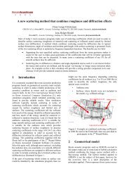
2. GEOMETRICAL MODEL
Room acoustic programs such as ODEON covered in this paper makes use of some kind of
hybrid calculation method combing the Image source method with a raytracing method. The
hybrid method applied in ODEON is not the subject of this paper, however for the overview
here is a short decription of the principles applied. Point responses from a point source can
be calculated by a hybrid method, which combines the image source method and a rayradiosity
method for early reflections below a specified reflection order with a special raytracing
/radiosity method for late reflections. The optimal reflection order (TO) at which the
model makes a transition from the early to the late method depends on the type of room. For
a more detailed description please see [6]. Typical values of TO are 1, 2 or 3, but in some
cases even a value of 0 may be preferred, in which case only the ray tracing algorithm is
used.
Energy
ISM
ESR
TO
RTM
Reflection order
Time
Figure 1:. Summary of the hybrid calculation method as used in ODEON. Early reflections below a selected
transition order (TO) are calculated using a combination of the image source method (ISM) and early
scattering rays (ESR). Above the TO, reflections are calculated using a ray-tracing method (RTM) which
includes scattering. In the special case where the TO is set to zero, the method becomes a ray-tracing model.
Note that all three methods will, most likely, overlap in time.

No matter the selected TO, the algorithm includes scattering, so for the simplicity we will in
the following assume that TO=0 was chosen; thus only the RTM( late ray-tracing) method is
described. Each time a ray hits /reflects from a surface, a secondary source is generated at the
point of incidence. The secondary source has strength and a time delay as calculated from the
total reflection path from the original source to the secondary source. Whether the secondary
source gives a contribution to the impulse response in a receiver point is determined from a
visibility check. Form the above can be derived that a ray which is reflected a 100 times
provides 100 secondary sources in the room, so potentially 1000 such rays may contribute as
much as 100000 reflections at a receiver depending on visibility.
Vector based scattering
Vector based scattering is an efficient way to include scattering in a ray tracing algorithm.
The direction of a reflected ray is calculated by adding the specular vector scaled by a factor
( 1−
s)
to a scattered vector (random direction, generated according to the Lambert
distribution [7]) which has been scaled by a factor s where s is the scattering coefficient. If
s is zero the ray is reflected in the specular direction, if it equals 1 then the ray is reflected in
a random direction. Often the resulting scatter coefficient may be in the range of say 0.02 to
0.20 and in this case rays will be reflected in directions which differ just slightly from the
specular one but this is enough to avoid artifacts due to simple geometrical reflection pattern.
Incident Specular (weight: 1-s)
Resulting
Scattered (weight: s)
Figure 2:Vector based scattering. Reflecting a ray from a surface with a scattering coefficient of 0.50 results in
a reflected direction which is the geometrical average of the specular direction and a random (scattered)
direction. Note: The scattering is a 3D phenomena, but here shown in 2D
3. THE REFLECTION BASED SCATTERING COEFFICIENT
In order to better include the diffraction phenomenon’s which is assumed to be vital to the
acoustics of class rooms, a new method for handling scattering has been developed for the
ODEON software [8]. The method takes into account that the amount of scattering caused by
diffraction is not fully known before the actual reflections are calculated because angles of
incidence, path-lengths etc. are not known before the calculations are carried out. In order to
allow such features to be included in predictions, we suggest the Reflection Based Scattering
coefficient s r which combines the surface roughness scattering coefficient s s with the
scattering coefficient due to diffraction s d that is calculated individually for each reflection
as calculations take place:
sr = 1− ( 1−
sd
) ⋅ ( 1−
ss
)
(1)

The formula calculates the fraction of energy which is not specular when both diffraction and
surface roughness is taken into account. ( 1 d ) s − denotes the energy which is not (edge)
diffracted, that is, energy reflected from the surface area either as specular energy or as
surface scattered energy, the resulting specular energy fraction from the surface
is ( 1−
sd ) ⋅ ( 1−
ss
) .
3.1 Ss, Surface Scattering
Surface scattering is in the following assumed to be scattering appearing due to random
surface roughness. This type of scattering gives rise to scattering which increase with
frequency. In figure 3 typical frequency functions are shown. In ODEON 8ß these functions
are used in the following way: The user may specify a scattering coefficient for the middle
frequency around 700 Hz (average of 500 – 1000 Hz bands), then ODEON expands that
coefficient into a value for each octave band, using interpolation or extrapolation.
Scattering coefficient
1
0,9
0,8
0,7
0,6
0,5
0,4
0,3
0,2
0,1
0
Sets of Scattering Coefficients
63 125 250 500 1000 2000 4000 8000
Frequency
0,015
0,06
0,25
0,55
0,8
0,9
Figure 3: Frequency functions for materials with different surface roughness. The legend of each scattering
coefficient curve denotes the scattering coefficient at 707 Hz.
3.2 Sd, Scattering Due to Diffraction
In order to estimate scattering due to diffraction, reflector theory is applied. The main theory
is presented in [9], the goal in that paper was to estimate the specular contribution of a
reflector with a limited area; given the basic dimensions of the surface, angle of incidence,
incident and reflected path lengths. Given the fraction of the energy which is reflected
specularily we can however also describe the fraction s d which has been scattered due to
diffraction. A short summary of the method is as follows: For a panel with the
dimensionsl ⋅ w ; above the upper limiting frequency f w (defined by the short dimension of
the panel) the frequency response can be simplified to be flat, i.e. that of an infinitely large
panel, below f w the response will fall off by 3 dB per octave. Below the second limiting
frequency f l (defined by the length of the panel), an additional 3 dB per octave is added
resulting in a fall off by 6 dB per octave. In the special case of a quadratic surface there will

only be one limiting frequency below which the specular component will decrease by 6 dB
per octave.
The attenuation factors l K and K w are estimates to the fraction of energy which is reflected
specularily. These factors take into account the incident and reflected path lengths (for ray
tracing we have to assume that reflected path length equals incident path length) and angle of
incidence. All information, which is not available before the calculation takes place.
f
w
K
w
⎧1
⎪
= ⎨ f
⎪
⎩ f w
c ⋅ a *
=
2(
w ⋅ cosθ
)
2
for
for
f
f
,
>
≤
f
f
w
w
f
l
,
c ⋅ a *
= 2
2 ⋅l
K
l
⎧1
⎪
= ⎨ f
⎪
⎩ f l
where
for
for
f
d
a*
=
2(
d
If we assume energy conservation then we must also assume that the energy which is not
reflected specularily has been diffracted - scattered due to diffraction. This leads to the
following formula for our scattering coefficient due to diffraction:
d
w
l
f
inc
inc
>
≤
f
f
⋅ d
l
l
refl
+ d
refl
)
(2)
(3)
s = 1 − K K
(4)
As can be seen, scattering caused by diffraction is a function of a number of parameters some
of which are not known before the actual calculation takes place. An example is that oblique
angle of incidence lead to increased scattering whereas parallel walls lead to low scattering
and sometimes flutter echoes. Another example is indicated by the characteristic distance a*,
if source or receiver is close to a surface, this surface may provide a specular reflection even
if its small, on the other hand, if far away it only provide scattered sound, s ≅ 1.
Log(E)
fl
fw
Log(frequency)
Figure 4: Energy reflected from a free suspended surface given the dimensions l ⋅ w . At high frequcies the
surface reflects energy specularily (red), at low frequencies, energy is assumed to be scattered (blue). f w is the
upper specular cutoff frequency defined by the shortest dimension of the surface, f is the lower cutoff
l
frequency which is defined by the length of the surface.
d

4. OBLIQUE LAMBERT
In the ray-tracing process a number of secondary sources are generated at the collision points
between walls and the rays traced. It has not been covered yet which directivity to assign to
these sources. A straight away solution, which is the method used in earlier versions of
ODEON, is to assign Lambert directivity patterns, that is the cosine directivity for diffuse
radiation. However the result is that the reflection from the secondary sources to the actual
receiver point is handled with 100 % scattering, no matter actual scattering properties for the
reflection. This is not the optimum solution, in fact when it comes to the reflection path from
wall to receiver we know not only the incident path length to the wall also the path length
from the wall to the receiver is available, allowing a better estimate of the characteristic
distance a * than was the case in the ray-tracing process where d refl was assumed to be equal
to d inc . So which directivity to assign to the secondary sources? We propose a directivity
pattern which we will call Oblique Lambert. Reusing the concept of Vector Based Scattering,
an orientation of our Oblique Lambert source can be obtained taking the Reflection Based
Scattering coefficient into account. If scattering is zero then the orientation of the Oblique
Lambert source is found by Snell’s Law. If the scattering coefficient is one then the
orientation is that of the traditional Lambert source and finally for all cases in-between the
orientation is determined by the vector found using the Vector Based Scattering method.
Shadow zone
Oblique angle
Figure 5: Traditional Lambert directivity to the left and Oblique Lambert to the right. Oblique Lambert
produces a shadow zone where no sound is reflected. The shadow zone is small if scattering is high or if the
incident direction is nearly perpendicular to the wall. On the other hand if scattering is low and the incident
direction is oblique then the shadow zone becomes large.
If Oblique Lambert was implemented as described without any further steps, this would lead
to an energy loss because part of the Lambert balloon is radiating energy out of the room. In
order to compensate for this, the directivity pattern has to be scaled with a factor which
accounts for the lost energy. If the angle is zero the factor is one and if the angle is 90° the
factor becomes its maximum of two because half of the balloon is outside the room. Factors
for angles between 0° and 90° have been found using numerical integration.
A last remark on Oblique Lambert is that it can include frequency depending scattering at
virtually no computational cost. This part of the algorithm does not involve any ray-tracing
which tends to be the heavy computational part in room acoustics prediction, only the
orientation of the Oblique Lambert source has to be recalculated for each frequency of
interest in order to model scattering as a function of frequency.

5. OPTIMAL SIZE OF SURFACE AND LEVEL OF DETAIL
Common questions with prediction programs based on geometrical assumptions are how
small surfaces should be included in models, which details should be included and which
should be omitted etc. Without a diffraction algorithm such as the one described above, risks
are that far away objects contribute with strong specular reflections when in fact the reflected
sound should be completely scattered. This results in decay curves with numerous spurious
spikes – this is no longer a problem with this novel algorithm. So which recommendations
should be given? The straight forward answer is that surfaces which look big from any
relevant source or receiver position should be modeled. If on the other hand the surfaces are
far away from sources and receivers then many small surfaces may be substituted with fewer
large ones. In this case one should however remember to compensate for details not modeled
by assigning appropriate higher scatting coefficients. Some geometries generated in CAD
programs such as AutoCAD may be subdivided into many small surfaces which are not
relevant for diffraction calculations. The geometry in the left side of figure 6 will not be
suited for the diffraction algorithms suggested. However an algorithm which can
automatically stitch such numerous small surfaces into fewer and larger ones better suited for
the diffraction handling has been developed. At the same time the stitched geometry is far
easier to handle when it comes to assigning surface properties and much better suited for
visualization and printouts. If the original model had been used, then scattering due to
diffraction would have been overestimated.
Odeon©1985-2005
X
Z
O
Y
Odeon©1985-2005
Figure 6: At the left a geometry which was imported from AutoCAD without stitching surfaces, at the right the
model which was imported in ODEON using the stitching algorithm (Glue surface option). The number of
surfaces was reduced from 1362 to 209 surfaces without any additional user interaction forming a geometry
compatible with the Reflection Based Scattering coefficient.
6. CASE STUDY
The following example illustrates the problems which occur when predicting acoustics in a
class room and similar rooms where the ceiling height is low and distribution of absorption is
very uneven. The room chosen for the case study is the lecture room at Acoustic Technology,
Ørsted-DTU. It is a box shaped room with the dimensions 9.46 x 6.69 x 3.00 metres,
measured average reverberation time was 0.44 seconds at 1000 Hz. The surfaces are: Walls
of painted brickwork, windows, wooden floor, blackboards, a wooden door, a suspended
ceiling with high absorption and furniture of wood. Virtually the whole range of absorption
coefficients is in use at mid-frequencies.
X
Z
O
Y

4
P1 1
3
3
2
2
Odeon©1985-2005
Figure 7: Model of the lecture room at Acoustic Technology, Ørsted-DTU. The room is a box shaped room with
the dimensions 9.46 x 6.69 x 3.00 metres, measured average reverberation time was 0.44 seconds at 1000 Hz.
Initial calculations were carried out with one source and seven receiver positions. The
materials were not fitted rather they were chosen from a library of ‘standard materials’
therefore may not reflect accurately the properties of the real materials; however the data
have sufficient accuracy in order to illustrate the problem. To limit the data presented in the
following, only reverberation time T30 at the 1000 Hz octave band is presented. Other
parameters may also be relevant, indeed one reason to use a prediction program such as
ODEON may be to predict parameters such as C80, D50 or STI or to be able to auralize the
acoustics of a room. However T30 illustrates the problem quite well.
T30 at 1000 Hz
5
4
3
2
1
0
Predicted RT, average of 7 positions
traditional scattering model
1
6
0 0,2 0,4 0,6 0,8 1
Scattering coefficient
Figure 8: Predicted reverberation time at 1000 Hz as function of scattering coefficient when a traditional
scattering model is used. For comparison the average of the measured reverberation time was 0.44 seconds and
the reverberation time predicted with the Sabine formula was 0.37 seconds
4
5
7

First set of calculations were carried out using a traditional scattering model where the userspecified
scattering coefficients should be large enough to account for scattering due to
limited surfaces size as well as scattering due to surface roughness. Calculations were carried
out using different scattering coefficients in order to find the magnitude of influence from the
choice of coefficient as well as to find the best choice. In order to keep things simple, the
same scattering coefficient was applied to all surfaces although it could be argued that larger
coefficients should be used for the smaller surfaces such as chairs and tables.
As can be seen the results are dramatically influenced by the scattering coefficient chosen,
when the scattering coefficient is set to zero, that is completely smooth walls, which are
considered infinitely large, the predicted reverberation time is very far away from the
measured Tavr = 0.
44 seconds. Scattering coefficients in the range of 0.25 to 0.5 seems to
provide predictions which correspond better with measured reverberation. These scattering
coefficients are in agreement with the findings in [4] where 0.3 was suggested, however the
scattering coefficient of 0.1 found by Lam [2] for large smooth surfaces in concert halls leads
to dramatic over estimation of the reverberation time.
In the second set of calculations the Reflection Based Scattering method was applied. In this
case no extreme results are found. It seems that best results are obtained when a scattering
coefficient between 0.05 and 0.10 is used. It should be recalled, that frequency dependent
scattering is actually applied, but only the mid-frequency value need to be specified. The
walls in the room consist of painted brickwork with filled joints a fairly but not completely
smooth material, Lab. measurement according to ISO/FDIS 17497-1 [10] of smooth
materials indicates that ss lies around 0.02-0.03 for the mid-frequencies [11] so this seems to
be a realistic choice. The predicted results where lower and higher scattering coefficients
were applied do not seem unrealistic.
T30 at 1000 Hz
0,7
0,6
0,5
0,4
0,3
0,2
0,1
0
Predicted RT, average of 7 positions
Reflection Based Scattering Model
0 0,2 0,4 0,6 0,8 1
Scattering coefficient
Figure 9: Predicted reverberation time at 1000 Hz as function of scattering coefficient when the Reflection
Based Scattering model is used. The measured reverberation time of 0.44 seconds indicates that a scattering
coefficient between 0.05 and 0.10 is optimum.

7. CONCLUSIONS
A novel method for modelling of scattering which combines the separate components of
frequency depending scattering due to surface roughness and diffraction was developed.
Initial evaluations do indicate that the scattering coefficients to be used with this method are
compatible with those obtained through measurements according to ISO/DIS 17497-1. Some
of the benefits are; less guesswork for the user of the prediction software, improved
predictions and less sensitivity to small surfaces, e.g. better compatibility with architects
CAD models.
8. REFERENCES
[1] Michael Vorländer, International Round Robin on Room Acoustical Computer Simulations, Trondheim,
Norway 1995.Proceedings Vol. II p. 689 - 692.
[2] Lam Y.W., "On the modelling of diffuse reflections in room acoustics prediction", Refereed Invited
Paper, Proc. BEPAC & EPSRC Conference on Sustainable Building, p.106-113, 1997.
[3] Ingolf Bork. A Comparison of Room Simulation Software – The 2 nd Round Robin on Room Acoustical
Computer Software. Acta Acoustica, Vol. 86(2000) p. 943-956.
[4] J. Heiden. ODEON Auralization Adapted to Reality. Baltic-Nordic Acoustical Meeting 25-28 August
2002.
[5] Murray Hodgson. Evidence of diffuse reflections in rooms. J. Acoust. Soc. Am. 89 (2), February 1991
[6] Claus Lynge Christensen, Odeon Room Acoustics Program, Version 7.0, User Manual, Industrial,
Auditorium and Combined Editions, Odeon A/S, Lyngby, Denmark, August 2004. (86 pages).
[7] J.H. Rindel, Computer Simulation Techniques for Acoustical Design of Rooms. Acoustics Australia
1995, Vol. 23 p. 81-86.
[8] Claus Lynge Christensen, The ODEON homepage, www.odeon.dk.
[9] J.H. Rindel. Acoustic Design of Reflectors in Auditoria. Proceedings, Institute of Acoustics 1992, Vol.
14: Part 2, p.119-128.
[10] Michel Vorländer, Jean-Jacques Embrects, Gerrit Vermeir, Márcio Henrique de Avelar Gomes. Case
Studies in Measurements of Random Incidence Scattering Coefficients. Acta Acoustica united with
Acoustica. Vol. 90 (2004), p. 858-867.
[11] ISO/FDIS 17497-1: Acoustics - Measurement of sound scattering properties of surfaces – Part 1:
Measurements of random-incidence scattering coefficients in a reverberation room. 2000.