Validation of turbine noise prediction tools with acoustic - MTU Aero ...

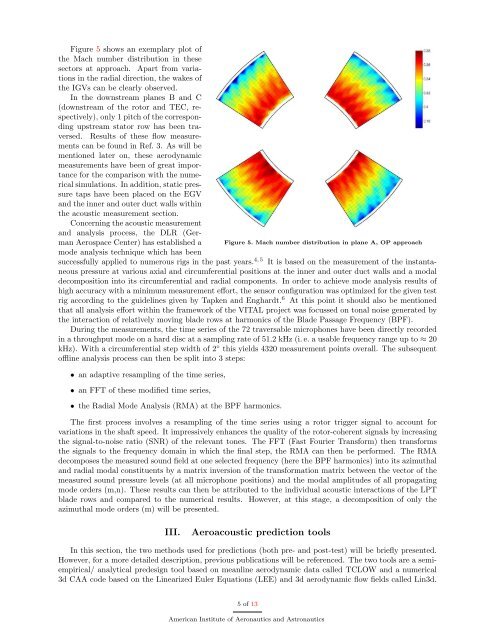
Figure 5 shows an exemplary plot of
the Mach number distribution in these
sectors at approach. Apart from variations
in the radial direction, the wakes of
the IGVs can be clearly observed.
In the downstream planes B and C
(downstream of the rotor and TEC, respectively),
only 1 pitch of the corresponding
upstream stator row has been traversed.
Results of these flow measurements
can be found in Ref. 3. As will be
mentioned later on, these aerodynamic
measurements have been of great importance
for the comparison with the numerical
simulations. In addition, static pressure
taps have been placed on the EGV
and the inner and outer duct walls within
the acoustic measurement section.
Concerning the acoustic measurement
and analysis process, the DLR (German
Aerospace Center) has established a Figure 5. Mach number distribution in plane A, OP approach
mode analysis technique which has been
successfully applied to numerous rigs in the past years. 4, 5 It is based on the measurement of the instantaneous
pressure at various axial and circumferential positions at the inner and outer duct walls and a modal
decomposition into its circumferential and radial components. In order to achieve mode analysis results of
high accuracy with a minimum measurement effort, the sensor configuration was optimized for the given test
rig according to the guidelines given by Tapken and Enghardt. 6 At this point it should also be mentioned
that all analysis effort within the framework of the VITAL project was focussed on tonal noise generated by
the interaction of relatively moving blade rows at harmonics of the Blade Passage Frequency (BPF).
During the measurements, the time series of the 72 traversable microphones have been directly recorded
in a throughput mode on a hard disc at a sampling rate of 51.2 kHz (i. e. a usable frequency range up to ≈ 20
kHz). With a circumferential step width of 2◦ this yields 4320 measurement points overall. The subsequent
offline analysis process can then be split into 3 steps:
• an adaptive resampling of the time series,
• an FFT of these modified time series,
• the Radial Mode Analysis (RMA) at the BPF harmonics.
The first process involves a resampling of the time series using a rotor trigger signal to account for
variations in the shaft speed. It impressively enhances the quality of the rotor-coherent signals by increasing
the signal-to-noise ratio (SNR) of the relevant tones. The FFT (Fast Fourier Transform) then transforms
the signals to the frequency domain in which the final step, the RMA can then be performed. The RMA
decomposes the measured sound field at one selected frequency (here the BPF harmonics) into its azimuthal
and radial modal constituents by a matrix inversion of the transformation matrix between the vector of the
measured sound pressure levels (at all microphone positions) and the modal amplitudes of all propagating
mode orders (m,n). These results can then be attributed to the individual acoustic interactions of the LPT
blade rows and compared to the numerical results. However, at this stage, a decomposition of only the
azimuthal mode orders (m) will be presented.
III. Aeroacoustic prediction tools
In this section, the two methods used for predictions (both pre- and post-test) will be briefly presented.
However, for a more detailed description, previous publications will be referenced. The two tools are a semiempirical/
analytical predesign tool based on meanline aerodynamic data called TCLOW and a numerical
3d CAA code based on the Linearized Euler Equations (LEE) and 3d aerodynamic flow fields called Lin3d.
5 of 13
American Institute of Aeronautics and Astronautics