Ordered/Ordinal Logistic Regression with SAS and Stata1 This ...
Ordered/Ordinal Logistic Regression with SAS and Stata1 This ...
Ordered/Ordinal Logistic Regression with SAS and Stata1 This ...

You also want an ePaper? Increase the reach of your titles
YUMPU automatically turns print PDFs into web optimized ePapers that Google loves.
<strong>Ordered</strong>/<strong>Ordinal</strong> <strong>Logistic</strong> <strong>Regression</strong> <strong>with</strong> <strong>SAS</strong> <strong>and</strong> Stata 1<br />
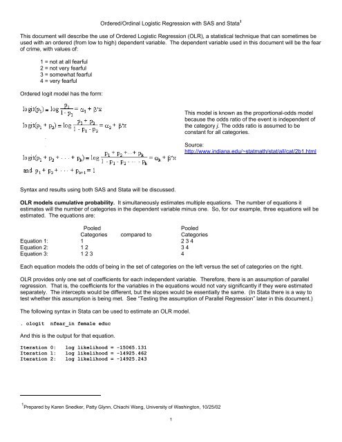
<strong>This</strong> document will describe the use of <strong>Ordered</strong> <strong>Logistic</strong> <strong>Regression</strong> (OLR), a statistical technique that can sometimes be<br />
used <strong>with</strong> an ordered (from low to high) dependent variable. The dependent variable used in this document will be the fear<br />
of crime, <strong>with</strong> values of:<br />
1 = not at all fearful<br />
2 = not very fearful<br />
3 = somewhat fearful<br />
4 = very fearful<br />
<strong>Ordered</strong> logit model has the form:<br />
Syntax <strong>and</strong> results using both <strong>SAS</strong> <strong>and</strong> Stata will be discussed.<br />
1 Prepared by Karen Snedker, Patty Glynn, Chiachi Wang, University of Washington, 10/25/02<br />
1<br />
<strong>This</strong> model is known as the proportional-odds model<br />
because the odds ratio of the event is independent of<br />
the category j. The odds ratio is assumed to be<br />
constant for all categories.<br />
Source:<br />
http://www.indiana.edu/~statmath/stat/all/cat/2b1.html<br />
OLR models cumulative probability. It simultaneously estimates multiple equations. The number of equations it<br />
estimates will the number of categories in the dependent variable minus one. So, for our example, three equations will be<br />
estimated. The equations are:<br />
Pooled Pooled<br />
Categories compared to Categories<br />
Equation 1: 1 2 3 4<br />
Equation 2: 1 2 3 4<br />
Equation 3: 1 2 3 4<br />
Each equation models the odds of being in the set of categories on the left versus the set of categories on the right.<br />
OLR provides only one set of coefficients for each independent variable. Therefore, there is an assumption of parallel<br />
regression. That is, the coefficients for the variables in the equations would not vary significantly if they were estimated<br />
separately. The intercepts would be different, but the slopes would be essentially the same. (In Stata there is a way to<br />
test whether this assumption is being met. See “Testing the assumption of Parallel <strong>Regression</strong>” later in this document.)<br />
The following syntax in Stata can be used to estimate an OLR model.<br />
. ologit nfear_in female educ<br />
And this is the output for that equation.<br />
Iteration 0: log likelihood = -15065.131<br />
Iteration 1: log likelihood = -14925.462<br />
Iteration 2: log likelihood = -14925.243
<strong>Ordered</strong> logit estimates Number of obs = 12261<br />
LR chi2(2) = 279.78<br />
Prob > chi2 = 0.0000<br />
Log likelihood = -14925.243 Pseudo R2 = 0.0093<br />
-----------------------------------------------------------------------------nfear_in<br />
| Coef. Std. Err. z P>|z| [95% Conf. Interval]<br />
-------------+---------------------------------------------------------------female<br />
| .5454657 .0336724 16.20 0.000 .4794691 .6114624<br />
educ | -.0180993 .0062164 -2.91 0.004 -.0302832 -.0059154<br />
-------------+----------------------------------------------------------------<br />
_cut1 | -1.11355 .0924472 (Ancillary parameters)<br />
_cut2 | .6022201 .092258<br />
_cut3 | 2.977691 .0984957<br />
------------------------------------------------------------------------------<br />
The syntax used to estimate the same OLR equation in <strong>SAS</strong> follows.<br />
And the results follow.<br />
The LOGISTIC Procedure<br />
Model Information<br />
Data Set SNEDKER<br />
Response Variable nfear_in fear<br />
Number of Response Levels 4<br />
Number of Observations 12261<br />
Model cumulative logit<br />
Optimization Technique Fisher's scoring<br />
Response Profile<br />
<strong>Ordered</strong> Total<br />
Value nfear_in Frequency<br />
1 4 641<br />
2 3 3858<br />
3 2 4793<br />
4 1 2969<br />
Probabilities modeled are cumulated over the lower <strong>Ordered</strong> Values.<br />
Model Convergence Status<br />
Convergence criterion (GCONV=1E-8) satisfied.<br />
Score Test for the Proportional Odds Assumption<br />
Chi-Square DF Pr > ChiSq<br />
252.5987 4
The LOGISTIC Procedure<br />
Testing Global Null Hypothesis: BETA=0<br />
Test Chi-Square DF Pr > ChiSq<br />
Likelihood Ratio 279.7770 2
URL provides information about calculating predicted probabilities <strong>with</strong> <strong>SAS</strong>.<br />
http://www.indiana.edu/~statmath/stat/all/cat/2b1.html<br />
For information on testing the model for explanatory power of a model, please refer to:<br />
http://www.ats.ucla.edu/stat/stata/library/logit_wgould.htm<br />
Testing the assumption of Parallel <strong>Regression</strong> (Drawn from <strong>Regression</strong> Models for Categorical Dependent Variables<br />
Using Stata, Long <strong>and</strong> Freese, 2001)<br />
J. Scott Long <strong>and</strong> Jeremy Freese have created an add-in file for Stata which allows the easy testing of the assumption of<br />
Parallel <strong>Regression</strong>. For complete information on how to install this ado file, see:<br />
http://www.indiana.edu/~jsl650/spostinstall.htm#Heading03<br />
Once you have installed these useful additions, estimate your <strong>Ordinal</strong> <strong>Logistic</strong> <strong>Regression</strong> model (for example):<br />
. ologit nfear_in female educ<br />
And then issue the comm<strong>and</strong>:<br />
. brant, detail<br />
You will get results like:<br />
Estimated coefficients from j-1 binary regressions<br />
y>1 y>2 y>3<br />
female .62821863 .48924177 .55179906<br />
educ .04872347 -.04745798 -.15864904<br />
_cons .14818344 -.16496036 -1.1202262<br />
Brant Test of Parallel <strong>Regression</strong> Assumption<br />
Variable | chi2 p>chi2 df<br />
-------------+--------------------------<br />
All | 256.77 0.000 4<br />
-------------+-------------------------female<br />
| 10.44 0.005 2<br />
educ | 250.30 0.000 2<br />
----------------------------------------<br />
A significant test statistic provides evidence that the parallel<br />
regression assumption has been violated.<br />
First you will see the results of each binary regression that was estimated when the OLR coefficients were calculated.<br />
These represent the equations represented above under the heading “OLR models cumulative probability”. The model<br />
" y>1" represents Equation 1, "y>2" is Equation 2, <strong>and</strong> "y>3" is Equation 4. (We proved this to ourselves by estimating<br />
logistic regression models for each of these.) For the Assumption of Parallel <strong>Regression</strong> to be true, the coefficients across<br />
these equations would not vary very much. But, in this example, they do vary. In fact, for education, the slope even<br />
changes directions. You are also provided <strong>with</strong> the results of a Chi-square test, which, in this case, shows that the parallel<br />
regression assumption has been violated. Note: <strong>This</strong> test is sensitive to the number of cases. Samples <strong>with</strong> larger<br />
numbers of cases are more likely to show a statistically significant test, <strong>and</strong> evidence that the parallel regression<br />
assumption has been violated.<br />
4