Worksheet 1, Math 126 Applications of Linear Approximation ...
Worksheet 1, Math 126 Applications of Linear Approximation ...
Worksheet 1, Math 126 Applications of Linear Approximation ...

You also want an ePaper? Increase the reach of your titles
YUMPU automatically turns print PDFs into web optimized ePapers that Google loves.
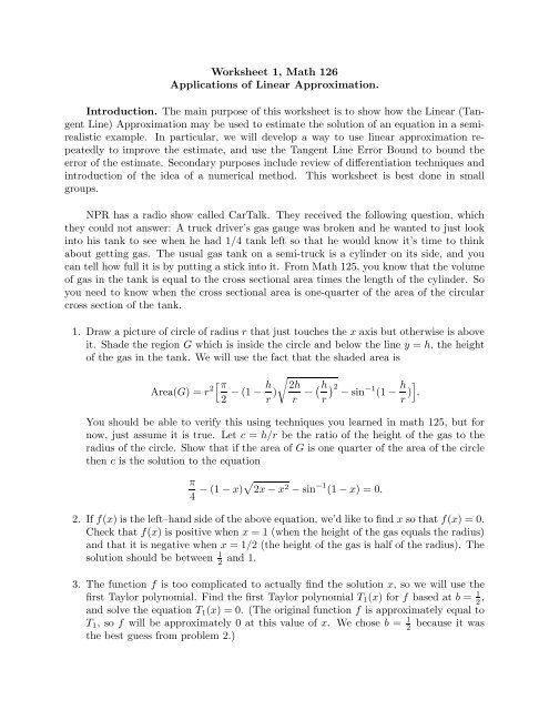
<strong>Worksheet</strong> 1, <strong>Math</strong> <strong>126</strong><br />
<strong>Applications</strong> <strong>of</strong> <strong>Linear</strong> <strong>Approximation</strong>.<br />
Introduction. The main purpose <strong>of</strong> this worksheet is to show how the <strong>Linear</strong> (Tangent<br />
Line) <strong>Approximation</strong> may be used to estimate the solution <strong>of</strong> an equation in a semirealistic<br />
example. In particular, we will develop a way to use linear approximation repeatedly<br />
to improve the estimate, and use the Tangent Line Error Bound to bound the<br />
error <strong>of</strong> the estimate. Secondary purposes include review <strong>of</strong> differentiation techniques and<br />
introduction <strong>of</strong> the idea <strong>of</strong> a numerical method. This worksheet is best done in small<br />
groups.<br />
NPR has a radio show called CarTalk. They received the following question, which<br />
they could not answer: A truck driver’s gas gauge was broken and he wanted to just look<br />
into his tank to see when he had 1/4 tank left so that he would know it’s time to think<br />
about getting gas. The usual gas tank on a semi-truck is a cylinder on its side, and you<br />
can tell how full it is by putting a stick into it. From <strong>Math</strong> 125, you know that the volume<br />
<strong>of</strong> gas in the tank is equal to the cross sectional area times the length <strong>of</strong> the cylinder. So<br />
you need to know when the cross sectional area is one-quarter <strong>of</strong> the area <strong>of</strong> the circular<br />
cross section <strong>of</strong> the tank.<br />
1. Draw a picture <strong>of</strong> circle <strong>of</strong> radius r that just touches the x axis but otherwise is above<br />
it. Shade the region G which is inside the circle and below the line y = h, the height<br />
<strong>of</strong> the gas in the tank. We will use the fact that the shaded area is<br />
Area(G) = r 2<br />
�<br />
π<br />
2<br />
h<br />
− (1 −<br />
r )<br />
�<br />
2h<br />
r<br />
�h �2 −1 h<br />
− − sin (1 −<br />
r<br />
r )<br />
�<br />
.<br />
You should be able to verify this using techniques you learned in math 125, but for<br />
now, just assume it is true. Let c = h/r be the ratio <strong>of</strong> the height <strong>of</strong> the gas to the<br />
radius <strong>of</strong> the circle. Show that if the area <strong>of</strong> G is one quarter <strong>of</strong> the area <strong>of</strong> the circle<br />
then c is the solution to the equation<br />
π<br />
4 − (1 − x)� 2x − x 2 − sin −1 (1 − x) = 0.<br />
2. If f(x) is the left–hand side <strong>of</strong> the above equation, we’d like to find x so that f(x) = 0.<br />
Check that f(x) is positive when x = 1 (when the height <strong>of</strong> the gas equals the radius)<br />
and that it is negative when x = 1/2 (the height <strong>of</strong> the gas is half <strong>of</strong> the radius). The<br />
and 1.<br />
solution should be between 1<br />
2<br />
3. The function f is too complicated to actually find the solution x, so we will use the<br />
first Taylor polynomial. Find the first Taylor polynomial T1(x) for f based at b = 1<br />
2 ,<br />
and solve the equation T1(x) = 0. (The original function f is approximately equal to<br />
T1, so f will be approximately 0 at this value <strong>of</strong> x. We chose b = 1 because it was<br />
2<br />
the best guess from problem 2.)
Newton’s Method. We’ve just seen an example <strong>of</strong> a problem in which we needed to<br />
find a value r (called a “zero” or “root”) such that f(r) = 0. For simple functions like linear<br />
or quadratic polynomials, there is a formula for the zeros. For more complicated functions<br />
f(x), usually no such formula is possible. We can replace f by its linear approximation, and<br />
find where the linear approximation equals zero as we did above. But for many practical<br />
problems, we need a more accurate approximation. The rest <strong>of</strong> this worksheet introduces a<br />
numerical method, Newton’s Method, for finding a zero <strong>of</strong> a function. Like most numerical<br />
methods, it gives an approximate answer whose accuracy can be improved by repeating<br />
similar calculations.<br />
4. Let f be a differentiable function. (You can think <strong>of</strong> the function f above as an<br />
example, but do the following calculations for the general case.) We are going to find<br />
the first Taylor polynomial for f based at a sequence <strong>of</strong> different points x1, x2, etc.<br />
Suppose x1 is given, and let T1(x) be the first Taylor polynomial for f based at b = x1.<br />
We will choose x2 to be the zero <strong>of</strong> T1 (and thus approximately a zero <strong>of</strong> f). Show<br />
that if T1(x2) = 0, then<br />
x2 = x1 − f(x1)<br />
f ′ (x1) .<br />
Discussion: Newton’s idea was to repeat this process. If x2 is approximately a zero<br />
<strong>of</strong> f, find the first Taylor polynomial based at b = x2. Then by the same reasoning as you<br />
just did to find x2, the new T1 will equal zero at<br />
x3 = x2 − f(x2)<br />
f ′ (x2) .<br />
Repeating the idea <strong>of</strong> step 3 for n = 1, 2, 3, . . ., set<br />
xn+1 = xn − f(xn)<br />
f ′ (xn) .<br />
Then the numbers x1, x2, x3, . . . should get closer and closer to a zero r <strong>of</strong> f, i.e. f(r) = 0.<br />
5. Let’s illustrate this with a simpler function, f(x) = x 2 −3, starting with x1 = 2. First<br />
draw the picture. Graph f and T1 based at b = 2, and label the zeros <strong>of</strong> f and the<br />
zero <strong>of</strong> T1. The zero <strong>of</strong> T1 is the x-value <strong>of</strong> the point where the tangent line to the<br />
graph <strong>of</strong> f crosses the x axis. Calculate this value.<br />
We can interpret your picture in the following way: We made a guess for the zero r <strong>of</strong><br />
f, in this case we guessed 2. Then the tangent line to the graph <strong>of</strong> f based at b = 2<br />
crosses the x axis at a point much closer to the zero <strong>of</strong> f than 2, namely at x2 = 1.75.<br />
In other words, we’ve improved our guess. Repeat this process starting with 1.75<br />
instead <strong>of</strong> 2: Graph the tangent line to the curve y = x 2 − 3 based at b = 1.75. (You<br />
may need to draw a new, larger scale graph.) Find where this line crosses the x-axis.<br />
This number, x3, should be even closer to √ 3 = 1.732 . . . .
6. We can use some algebra and a calculator to find the sequence<br />
xn+1 = xn − f(xn)<br />
f ′ (xn) .<br />
If f(x) = x 2 − 3, we can simplify the right side to<br />
xn+1 = xn<br />
2<br />
3<br />
+ .<br />
2xn<br />
Set x1 = 2, and use your calculator to find x2, x3, x4 and x5. Notice that these<br />
numbers are getting close to √ 3, which is a zero <strong>of</strong> f.<br />
7. Now we return to the general case to discuss the accuracy <strong>of</strong> x1, x2, x3, ..., xn as<br />
approximations for a zero <strong>of</strong> f. Suppose that we are given a function f and an initial<br />
guess b for a zero <strong>of</strong> f. Let c = b − f(b)/f ′ (b). Suppose f(r) = 0 and suppose that I<br />
is an interval containing r, b and c. Suppose also that |f ′′ (x)| ≤ M and |f ′ (x)| ≥ K<br />
for all x in the interval I. Use the Tangent Line Error Bound for f based at b (setting<br />
x = r) to show that<br />
|c − r| ≤ M<br />
2K |b − r|2 .<br />
We can apply this error bound at each stage <strong>of</strong> Newton’s method. The error bound<br />
means that if the error in the guess (xn) for the zero (r) at stage n is at most 10 −m ,<br />
then the error at stage n + 1 is at most (M/2K)10 −2m . In other words, the number<br />
<strong>of</strong> correct digits roughly doubles at each step. This is remarkably fast convergence!<br />
How many digits are correct in x1, x2, x3, x4, and x5 in problem 5 above?<br />
Some concluding remarks. Applying Newton’s method to the gas tank problem<br />
is a bit more complicated than the calculations you have just done, and you are probably<br />
running out <strong>of</strong> time in this quiz section. From the simpler example <strong>of</strong> f(x) = x 2 − 3, you<br />
can see how Newton’s Method gives a good approximation <strong>of</strong> the zero <strong>of</strong> a function, and<br />
how the error bound decreases dramatically after each successive step. More important<br />
applications include, for example, solving Kepler’s equation which arises in the study <strong>of</strong><br />
planetary motion. Some calculators have a “Solve” button which is used to find a zero, that<br />
is, solve an equation. These calculators use Newton’s method, except that the derivative<br />
is estimated by difference quotients instead <strong>of</strong> computed analytically. If you have time at<br />
home, test your understanding by applying a few steps <strong>of</strong> Newton’s method to the gas<br />
tank problem. Check your work by evaluating f at each step. The values f(xn) should<br />
become very small, and the number <strong>of</strong> digits <strong>of</strong> xn which are the same as the digits <strong>of</strong> the<br />
root r should roughly double at each step.<br />
A listener to CarTalk suggested a quick approximate solution to the gas tank problem.<br />
Drink a can <strong>of</strong> pop until there is 1/4 left. You can measure the depth with a straw when<br />
the can is standing up. Then turn the can on its side and measure the depth <strong>of</strong> the pop<br />
and find the ratio with the radius (half <strong>of</strong> the diameter) <strong>of</strong> the can. This gives a rough<br />
approximation for the ratio the truck driver should use (about 3:5).