THE SQUARE-ROOT UNSCENTED KALMAN FILTER FOR STATE ...

THE SQUARE-ROOT UNSCENTED KALMAN FILTER
FOR STATE AND PARAMETER-ESTIMATION
Rudolph van der Merwe and Eric A. Wan
Oregon Graduate Institute of Science and Technology
20000 NW Walker Road, Beaverton, Oregon 97006, USA
�rvdmerwe,ericwan�@ece.ogi.edu
ABSTRACT
Over the last 20-30 years, the extended Kalman filter (EKF) has
become the algorithm of choice in numerous nonlinear estimation
and machine learning applications. These include estimating the
state of a nonlinear dynamic system as well estimating parameters
for nonlinear system identification (e.g., learning the weights of
a neural network). The EKF applies the standard linear Kalman
filter methodology to a linearization of the true nonlinear system.
This approach is sub-optimal, and can easily lead to divergence.
Julier et al. [1] proposed the unscented Kalman filter (UKF) as
a derivative-free alternative to the extended Kalman filter in the
framework of state-estimation. This was extended to parameterestimation
by Wan and van der Merwe [2, 3]. The UKF consistently
outperforms the EKF in terms of prediction and estimation
error, at an equal computational complexity of Ç Ä 1 for general
state-space problems. When the EKF is applied to parameterestimation,
the special form of the state-space equations allows
for an Ç Ä implementation. This paper introduces the squareroot
unscented Kalman filter (SR-UKF) which is also Ç Ä for
general state-estimation and Ç Ä for parameter estimation (note
the original formulation of the UKF for parameter-estimation was
Ç Ä ). In addition, the square-root forms have the added benefit
of numerical stability and guaranteed positive semi-definiteness of
the state covariances.
1. INTRODUCTION
The EKF has been applied extensively to the field of nonlinear estimation
for both state-estimation and parameter-estimation. The
basic framework for the EKF (and the UKF) involves estimation of
the state of a discrete-time nonlinear dynamic system,
� � � �� � � (1)
Ý� � À Ü� Ò�� (2)
where � represent the unobserved state of the system, � is a
known exogenous input, and � is the observed measurement signal.
The process noise Ú� drives the dynamic system, and the observation
noise is given by Ò�. The EKF involves the recursive
estimation of the mean and covariance of the state under a Gaussian
assumption.
In contrast, parameter-estimation, sometimes referred to as system
identification, involves determining a nonlinear mapping � �
This work was sponsored in part by NSF under grant grant IRI-
9712346, ECS-0083106, and DARPA under grant F33615-98-C-3516.
1 Ä is the dimension of the state variable.
� Ü�� Û ,whereÜ� is the input, Ý� is the output, and the nonlinear
map, � ¡ , is parameterized by the vector Û. Typically, a training
set is provided with sample pairs consisting of known input and
desired outputs, ��� ���. The error of the machine is defined as
�� � �� � Ü�� Û , and the goal of learning involves solving
for the parameters Û in order to minimize the expectation of some
given function of the error. While a number of optimization approaches
exist (e.g., gradient descent and Quasi-Newton methods),
parameters can be efficiently estimated on-line by writing a new
state-space representation
Û� � Û� Ö� (3)
�� � � �� � ��� (4)
where the parameters Û� correspond to a stationary process with
identity state transition matrix, driven by process noise Ö� (the
choice of variance determines convergence and tracking performance).
The output �� corresponds to a nonlinear observation on
Û�. The EKF can then be applied directly as an efficient “secondorder”
technique for learning the parameters [4].
2. THE UNSCENTED KALMAN FILTER
The inherent flaws of the EKF are due to its linearization approach
for calculating the mean and covariance of a random variable which
undergoes a nonlinear transformation. As shown in shown in [1,
2, 3], the UKF addresses these flaws by utilizing a deterministic
“sampling” approach to calculate mean and covariance terms. Essentially,
Ä ,sigma points (Ä is the state dimension), are chosen
based on a square-root decomposition of the prior covariance.
These sigma points are propagated through the true nonlinearity,
without approximation, and then a weighted mean and covariance
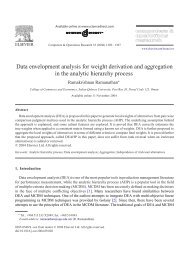
is taken. A simple illustration of the approach is shown in Figure
1 for a 2-dimensional system: the left plot shows the true mean
and covariance propagation using Monte-Carlo sampling; the center
plots show the results using a linearization approach as would be
done in the EKF; the right plots show the performance of the new
“sampling” approach (note only 5 sigma points are required). This
approach results in approximations that are accurate to the third
order (Taylor series expansion) for Gaussian inputs for all nonlinearities.
For non-Gaussian inputs, approximations are accurate to
at least the second-order [1]. In contrast, the linearization approach
of the EKF results only in first order accuracy.
The full UKF involves the recursive application of this “sampling”
approach to the state-space equations. The standard UKF
implementation is given in Algorithm 2.1 for state-estimation, and
uses the following variable definitions: ��� is a set of scalar
weights (Ï Ñ � �� Ä � , Ï � �� Ä � « ¬ ,

Actual (sampling) Linearized (EKF) UKF UT
Ý � � Ü
mean
true mean
covariance
true covariance
� Ì È Ü�
�Ý � � �Ü
ÈÝ � � Ì ÈÜ�
� �Ü
sigma points
0000 1111
UKF UT mean
0000 1111
� � � �
weighted sample mean
and covariance
UKF 00000 11111
UT covariance
01
11111
000000
10
1
01
01
01
0000 1111
0000 1111
0000 1111
0000 1111
0000 1111
transformed
sigma points
Figure 1: Example of mean and covariance propagation. a) actual,
b) first-order linearization (EKF), c) new “sampling” approach (UKF).
Ï Ñ
� � Ï� � �� Ä � � � � ����� Ä). � � Ô « Ä
� Ä and ­ � Ä � are scaling parameters. The constant «
determines the spread of the sigma points around �Ü and is usually
set to � � � « � . � is a secondary scaling parameter 2 . ¬
is used to incorporate prior knowledge of the distribution of Ü (for
Gaussian distributions, ¬ � is optimal). Also note that we define
the linear algebra operation of adding a column vector to a matrix,
i.e. � ¦ Ù as the addition of the vector to each column of the matrix.
The superior performance of the UKF over the EKF has been
demonstrated in a number of applications [1, 2, 3]. Furthermore,
unlike the EKF, no explicit derivatives (i.e., Jacobians or Hessians)
need to be calculated.
3. EFFICIENT SQUARE-ROOT IMPLEMENTATION
The most computationally expensive operation in the UKF corresponds
to calculating the new set of sigma points at each time
update. This requires taking a matrix square-root of the state covariance
matrix 3 , È Ê Ä¢Ä ,givenbyËË Ì � È. An efficient
implementation using a Cholesky factorization requires in general
Ç Ä �� computations [5]. While the square-root of È is an integral
part of the UKF, it is still the full covariance È which is recursively
updated. In the SR-UKF implementation, Ë will be propagated
directly, avoiding the need to refactorize at each time step.
The algorithm will in general still beÇ Ä , but with improved numerical
properties similar to those of standard square-root Kalman
filters [6]. Furthermore, for the special state-space formulation of
parameter-estimation, an Ç Ä implementation becomes possible.
The square-root form of the UKF makes use of three linear
algebra techniques[5] nl. QR decomposition, Cholesky factor updating
and efficient least squares, which we briefly review below:
¯ QR decomposition. The QR decomposition or factorization
of a matrix � Ê Ä¢Æ is given by, � Ì � ÉÊ, where
É Ê Æ¢Æ is orthogonal, Ê Ê Æ¢Ä is upper triangular
and Æ � Ä. The upper triangular part of Ê, � Ê,is
2We usually set � to
estimation [1].
for state-estimation and to Ä for parameter
3For notational clarity, the time index � has been omitted.
Initialize with:
�Ü � ��Ü ℄ È � �� Ü �Ü Ü �Ü Ì ℄ (5)
For � � ����� �,
Calculate sigma points:
� �
�
� �Ü� �Ü� ­ Ô È� �Ü� ­ Ô È�
Time update:
� £
��� � ��� � � Ù� ℄ (7)
�Ü
� �
��
�
�
È � �
5� ���
�� �
� �Ü �
Ï Ñ
�
� £
�����
Ï� �� £
£
����� �Ü � ℄�� ����� �Ü � ℄Ì Ê Ú
�Ü
�
���� � À�� ��� ℄
�Ý
� �
��
�
Measurement update equations:
�� �� �
ÈÜ�Ý� �
��
��
�
�
Ã� � ÈÜ�Ý� È
�� ��
�Ü� � �Ü
�
Õ
­ È �
�Ü
� ­
Õ
È �
�
�
(6)
(8)
(9)
Ï Ñ
� ������ (10)
Ï � ������� �Ý
� ℄������� �Ý
� ℄Ì Ê Ò
Ï � ������� �Ü
� ℄������� �Ý
� ℄Ì
Ã� Ý� �Ý
�
È� � È � Ã�È�Ý��Ý�ÃÌ �
where Ê Ú =process noise cov., Ê Ò =measurement noise cov.
Algorithm 2.1: Standard UKF algorithm.
(11)
(12)
(13)
(14)
the transpose of the Cholesky factor of È � �� Ì , i.e.,
�Ê � Ë Ì , such that � Ê Ì � Ê � �� Ì . Weusetheshorthand
notation qr�¡� to donate a QR decomposition of a matrix
where only � Ê is returned. The computational complexity
of a QR decomposition is Ç ÆÄ . Note that performing a
Cholesky factorization directly on È � �� Ì is Ç Ä ��
plus Ç ÆÄ to form �� Ì .
¯ Cholesky factor updating. If Ë is the original Cholesky factor
of È � �� Ì , then the Cholesky factor of the rank-
1 update (or downdate) È ¦ Ô �ÙÙ Ì is denoted as Ë �
cholupdate�Ë� Ù�¦��. If Ù is a matrix and not a vector,
then the result is Å consecutive updates of the Cholesky
factor using the Å columns of Ù. This algorithm (available
in Matlab as cholupdate) is only Ç Ä per update.
¯ Efficient least squares. The solution to the equation
�� Ì Ü � � Ì � also corresponds to the solution of the
overdetermined least squares problem �Ü � �. This can be
solved efficiently using a QR decomposition with pivoting

(implemented in Matlab’s ’/’ operator).
The complete specification of the new square-root filters is
given in Algorithm 3.1 for state-estimation and 3.2 for paramaterestimation.
Below we describe the key parts of the square-root
algorithms, and how they contrast with the stardard implementations.
Square-Root State-Estimation: As in the original UKF, the
filter is initialized by calculating the matrix square-root of the state
covariance once via a Cholesky factorization (Eqn. 16). However,
the propagted and updated Cholesky factor is then used in subsequent
iterations to directly form the sigma points. In Eqn. 20
the time-update of the Cholesky factor, Ë , is calculated using a
QR decompostion of the compound matrix containing the weighted
propagated sigma points and the matrix square-root of the additive
process noise covariance. The subsequent Cholesky update (or
downdate) in Eqn. 21 is necessary since the the zero’th weight,
Ï , may be negative. These two steps replace the time-update
of È in Eqn. 8, and is also Ç Ä .
The same two-step approach is applied to the calculation of
the Cholesky factor, Ë�Ý, of the observation-error covariance in
Eqns. 25 and 26. This step is Ç ÄÅ ,whereÅis the observation
dimension. In contrast to the way the Kalman gain is calculated
in the standard UKF (see Eqn. 12), we now use two nested
inverse (or least squares) solutions to the following expansion of
Eqn. 12, Ã� Ë�Ý� ËÌ�Ý� � ÈÜ�Ý� . Since Ë�Ý is square and triangular,
efficient “back-substitutions” can be used to solve for Ã�
directly without the need for a matrix inversion.
Finally, the posterior measurement update of the Cholesky factor
of the state covariance is calculated in Eqn. 30 by applying Å
sequential Cholesky downdates to Ë � . The downdate vectors are
the columns of Í � Ã�Ë�Ý� . This replaces the posterior update of
È� in Eqn. 14, and is also Ç ÄÅ .
Square-Root Parameter-Estimation: The parameter-estimation
algorithm follows a similar framework as that of the state-estimation
square-root UKF. However, an Ç ÅÄ algorithm, as opposed to
Ç Ä , is possible by taking advantage of the linear state transition
function. Specifically, the time-update of the state covariance
is given simply by È Û� � ÈÛ� Ê Ö � . Now, if we apply an
exponential weighting on past data 4 , the process noise covariance
is given by Ê Ö � � � ÊÄË ÈÛ� , and the time update of the
state covariance becomes,
È Û� � ÈÛ� � ÊÄË ÈÛ� � � ÊÄËÈÛ� � (15)
�
This translates readily into the factored form, Ë Û�
� � ÊÄË ËÛ�
(see Eqn. 33), and avoids the costlyÇ Ä QR and Cholesky based
updates necessary in the state-estimation filter. This Ç ÅÄ time
update step has recently been expanded by the authors to deal with
arbitrary diagonal noise covariance structures [7].
4. EXPERIMENTAL RESULTS
The improvement in error performance of the UKF over that of the
EKF for both state and parameter-estimation is well documented
[1, 2, 3]. The focus of this section will be to simply verify the
equivalent error performance of the UKF and SR-UKF, and show
the reduction in computational cost achieved by the SR-UKF for
4 This is identical to the approach used in weighted recursive least
squares (W-RLS). �ÊÄË is a scalar weighting factor chosen to be slightly
less than 1, i.e. �ÊÄË � �����.
5 Redraw sigma points to incorporate effect of process noise.
Initialize with:
�Ü � ��Ü ℄ Ë � chol
For � � ����� �,
Ò Ó
Ì
�� Ü �Ü Ü �Ü ℄
(16)
Sigma point calculation and time update:
� � ���Ü� �Ü� ­Ë� �Ü� ­Ë�℄ (17)
� £
��� � ��� � � Ù� ℄ (18)
�Ü
� �
�
Ï Ñ
�
� £
�����
(19)
��
��Õ
£ ¡ Ô ��
Ë � � qr Ï � � Ä���� �Ü � ÊÚ (20)
Ò Ó
£
Ë � � cholupdate Ë � � � �� �Ü � � Ï (21)
¢ £
5 � ��� � �Ü � �Ü � ­Ë � �Ü � ­Ë �
(22)
� ��� � À�� ��� ℄ (23)
�Ý
� �
��
�
Ï Ñ
� ������ (24)
Measurement update equations:
��Õ
� qr Ï �� � Ä�� �Ý�℄
��
��
ÈÜ�Ý� �
� cholupdate
��
�
Ô Ê Ò �
Ò Ë�Ý� � � �� �Ý� � Ï
��
Ï � ������� �Ü
� ℄������� �Ý
� ℄Ì
Ó
(25)
(26)
(27)
Ã� � ÈÜ�Ý� �ËÌ �Ý� �Ë�Ý� (28)
�Ü� � �Ü
�
Í � Ã�Ë�Ý�
Ã� Ý� �Ý
�
Ë� � cholupdate ¨ Ë
�
� Í � -1©
where Ê Ú =process noise cov., Ê Ò =measurement noise cov.
Algorithm 3.1: Square-Root UKF for state-estimation.
(29)
(30)
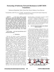
parameter-estimation. Figure 2 shows the superior performance of
UKF and SR-UKF compared to that of the EKF on estimating the
Mackey-Glass-30 chaotic time series corrupted by additive white
noise (3dB SNR). The error performance of the SR-UKF and UKF
are indistinguishable and are both superior to the EKF. The computational
complexity of all three filters are of the same order but the
SR-UKF is about 20% faster than the UKF and about 10% faster
than the EKF.
The next experiment shows the reduction in computational cost
achieved by the square-root unscented Kalman filters and how that
compares to the computational complexity of the EKF for parameterestimation.
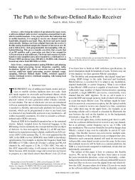
For this experiment, we use an EKF, UKF and SR-UKF
to train a 2-12-2 MLP neural network on the well known Mackay-
Robot-Arm 6 benchmark problem of mapping the joint angles of a
robot arm to the Cartesian coordinates of the hand. The learning
curves (mean square error (MSE) vs. learning epoch) of the different
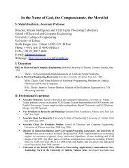
filters are shown in Figure 3. Figure 4 shows how the com-
6 http://wol.ra.phy.cam.ac.uk/mackay

Initialize with:
�Û � ��Û℄ ËÛ � chol
For � � ����� �,
Time update and sigma point calculation:
Ò Ó
Ì
�� Û �Û Û �Û ℄ (31)
�Û
� � �Û� (32)
�
Ë Û�
� � ÊÄË ËÛ�
¢
Ï ��� � �Û � �Û � ­Ë Û�
(33)
�Û
£
� ­Ë Û� (34)
���� � ��Ü�� Ï ��� ℄ (35)
��� �
��
Measurement update equations:
��Õ �
� qr Ï � � Ä�� � ��
��
��
ÈÛ��� �
�
� cholupdate
��
�
Ï Ñ
� ������ (36)
� Ô ��
Ê� Ò
Ë�� � � �� � Ó
�� � Ï
Ï � �Ï����� �Û
� ℄������� � ��℄ Ì
(37)
(38)
(39)
Ã� � ÈÛ��� �ËÌ �� �Ë�� (40)
�Û� � �Û � Ã� �� � �� (41)
Í � Ã�Ë��
(42)
ËÛ� � cholupdate ¨ Ë Û� � Í � -1©
(43)
where Ê � =measurement noise cov (this can be set to an arbitrary
value, e.g., ��Á.)
Algorithm 3.2: Square-Root UKF for parameter-estimation.
x(k)
x(k)
5
0
Estimation of Mackey−Glass time series : EKF
clean
noisy
EKF
−5
850 900 950 1000
k
Estimation of Mackey−Glass time series : UKF & SR−UKF
5
clean
noisy
UKF
SR−UKF
0
−5
850 900 950 1000
k
Figure 2: Estimation of the Mackey-Glass chaotic time-series (modeled
by a neural network) with the EKF, UKF and SR-UKF.
putational complexity of the different filters scale as a function of
the number of parameters (weights in neural network). While the
standard UKF is Ç Ä , both the EKF and SR-UKF are Ç Ä .
MSE
10 0
10 −1
10 −2
10 −3
Learning Curves : NN parameter estimation
EKF
UKF
SR−UKF
5 10 15 20 25
epoch
30 35 40 45 50
Figure 3: Learning curves for Mackay-Robot-Arm neural network
parameter-estimation problem.
flops
2
1.5
1
0.5
x 10 10
EKF
UKF
SR−UKF
Computational Complexity Comparison
100 200 300 400 500 600
number of parameters (L)
Figure 4: Computational complexity (flops/epoch) of EKF, UKF and
SR-UKF for parameter-estimation (Mackay-Robot-Arm problem).
5. CONCLUSIONS
The UKF consistently performs better than or equal to the well
known EKF, with the added benefit of ease of implementation in
that no analytical derivatives (Jacobians or Hessians) need to be
calculated. For state-estimation, the UKF and EKF have equal
complexity and are in general Ç Ä . In this paper, we introduced
square-root forms of the UKF. The square-root UKF has better
numerical properties and guarantees positive semi-definiteness
of the underlying state covariance. In addition, for parameterestimation
an efficient Ç Ä implementation is possible for the
square-root form, which is again of the same complexity as efficient
EKF parameter-estimation implementations.
6. REFERENCES
[1] S. J. Julier and J. K. Uhlmann, “A New Extension of the
Kalman Filter to Nonlinear Systems,” in Proc. of AeroSense:
The 11th Int. Symp. on Aerospace/Defence Sensing, Simulation
and Controls., 1997.
[2] E. Wan, R. van der Merwe, and A. T. Nelson, “Dual Estimation
and the Unscented Transformation,” in Neural Information
Processing Systems 12. 2000, pp. 666–672, MIT Press.
[3] E. A. Wan and R. van der Merwe, “The Unscented Kalman
Filter for Nonlinear Estimation,” in Proc. of IEEE Symposium
2000 (AS-SPCC), Lake Louise, Alberta, Canada, Oct. 2000.
[4] G.V. Puskorius and L.A. Feldkamp, “Decoupled Extended
Kalman Filter Training of Feedforward Layered Networks,” in
IJCNN, 1991, vol. 1, pp. 771–777.
[5] W. H. Press, S. A. Teukolsky, W. T. Vetterling, and B. P. Flannery,
Numerical Recipes in C : The Art of Scientific Computing,
Cambridge University Press, 2 edition, 1992.
[6] A. H. Sayed and T. Kailath, “A State-Space Approach to
Adaptive RLS Filtering,” IEEE Sig. Proc. Mag., July 1994.
[7] R. van der Merwe and E. A. Wan, “Efficient Derivative-Free
Kalman Filters for Online Learning,” in ESANN, Bruges, Belgium,
Apr. 2001.