Data envelopment analysis for weight derivation and aggregation in ...
Data envelopment analysis for weight derivation and aggregation in ...
Data envelopment analysis for weight derivation and aggregation in ...

Create successful ePaper yourself
Turn your PDF publications into a flip-book with our unique Google optimized e-Paper software.
Computers & Operations Research 33 (2006) 1289–1307<br />
www.elsevier.com/locate/cor<br />
<strong>Data</strong> <strong>envelopment</strong> <strong>analysis</strong> <strong>for</strong> <strong>weight</strong> <strong>derivation</strong> <strong>and</strong> <strong>aggregation</strong><br />
<strong>in</strong> the analytic hierarchy process<br />
Ramakrishnan Ramanathan ∗<br />
College of Commerce <strong>and</strong> Economics, Sultan Qaboos University, Post Box 20, Postal Code 123, Oman<br />
Available onl<strong>in</strong>e 11 November 2004<br />
Abstract<br />
<strong>Data</strong> <strong>envelopment</strong> <strong>analysis</strong> (DEA) is proposed <strong>in</strong> this paper to generate local <strong>weight</strong>s of alternatives from pair-wise<br />
comparison judgment matrices used <strong>in</strong> the analytic hierarchy process (AHP). The underly<strong>in</strong>g assumption beh<strong>in</strong>d<br />
the approach is expla<strong>in</strong>ed, <strong>and</strong> some salient features are explored. It is proved that DEA correctly estimates the<br />
true <strong>weight</strong>s when applied to a consistent matrix <strong>for</strong>med us<strong>in</strong>g a known set of <strong>weight</strong>s. DEA is further proposed to<br />
aggregate the local <strong>weight</strong>s of alternatives <strong>in</strong> terms of different criteria to compute f<strong>in</strong>al <strong>weight</strong>s. It is proved further<br />
that the proposed approach, called DEAHP <strong>in</strong> this paper, does not suffer from rank reversal when an irrelevant<br />
alternative(s) is added or removed.<br />
2004 Elsevier Ltd. All rights reserved.<br />
Keywords: Analytic hierarchy process; <strong>Data</strong> <strong>envelopment</strong> <strong>analysis</strong>; Aggregation; Independence of irrelevant alternatives<br />
1. Introduction<br />
<strong>Data</strong> <strong>envelopment</strong> <strong>analysis</strong> (DEA) is one of the most popular tools <strong>in</strong> production management literature<br />
<strong>for</strong> per<strong>for</strong>mance measurement, while the analytic hierarchy process (AHP) is a popular tool <strong>in</strong> the field<br />
of multiple-criteria decision-mak<strong>in</strong>g (MCDM). MCDM has been succ<strong>in</strong>ctly def<strong>in</strong>ed as mak<strong>in</strong>g decisions<br />
<strong>in</strong> the face of multiple conflict<strong>in</strong>g objectives [1]. Many researchers have found similarities between<br />
DEA <strong>and</strong> MCDM techniques. One of the earliest attempts to <strong>in</strong>tegrate DEA with multi-objective l<strong>in</strong>ear<br />
programm<strong>in</strong>g (a MCDM technique) was provided by Golany [2]. S<strong>in</strong>ce then, there have been several<br />
attempts to use the pr<strong>in</strong>ciples of DEA <strong>in</strong> the MCDM literature. The traditional goals of DEA <strong>and</strong> MCDM<br />
∗ Tel.: +968 513 333 X2849; fax: +968 514 043.<br />
E-mail address: ramanathan@squ.edu.om (R. Ramanathan).<br />
0305-0548/$ - see front matter 2004 Elsevier Ltd. All rights reserved.<br />
doi:10.1016/j.cor.2004.09.020
1290 R. Ramanathan / Computers & Operations Research 33 (2006) 1289–1307<br />
have been compared by Stewart [3]. The goal of DEA is to determ<strong>in</strong>e the productive efficiency of a system<br />
or decision-mak<strong>in</strong>g-unit (DMU) by compar<strong>in</strong>g how well the DMU converts <strong>in</strong>puts <strong>in</strong>to outputs, while the<br />
goal of MCDM is to rank <strong>and</strong> select from a set of alternatives that have conflict<strong>in</strong>g criteria. It has been<br />
recognized <strong>for</strong> more than a decade that the MCDM <strong>and</strong> DEA <strong>for</strong>mulations co<strong>in</strong>cide if <strong>in</strong>puts <strong>and</strong> outputs<br />
can be viewed as criteria <strong>for</strong> per<strong>for</strong>mance evaluation, with m<strong>in</strong>imization of <strong>in</strong>puts <strong>and</strong>/or maximization<br />
of outputs as associated objectives. [3–5]<br />
It is not the <strong>in</strong>tention <strong>in</strong> this paper to go <strong>in</strong>to the details of similarities. Interested readers are referred to<br />
recent reviews of multicriteria methods [6,7], books [8,9], <strong>and</strong> other related articles <strong>in</strong>clud<strong>in</strong>g those cited<br />
above [10–12]. This paper is concerned about us<strong>in</strong>g the concepts of DEA <strong>for</strong> address<strong>in</strong>g specific problems<br />
<strong>in</strong> the AHP [13], a popular technique of MCDM. The paper beg<strong>in</strong>s with brief discussions on DEA <strong>and</strong><br />
AHP <strong>and</strong> a literature survey on previous approaches l<strong>in</strong>k<strong>in</strong>g the two methods. The proposed approach<br />
synthesiz<strong>in</strong>g DEA concepts <strong>in</strong> AHP is discussed <strong>and</strong> illustrated <strong>in</strong> Section 3. Some of the salient features<br />
of the proposed approach are discussed <strong>in</strong> more detail <strong>in</strong> Section 4. The paper ends with a summary <strong>and</strong><br />
conclusions of the paper.<br />
2. The methodologies: DEA <strong>and</strong> AHP<br />
2.1. <strong>Data</strong> <strong>envelopment</strong> <strong>analysis</strong><br />
DEA has been successfully employed <strong>for</strong> assess<strong>in</strong>g the relative per<strong>for</strong>mance of a set of firms, usually<br />
called the DMU, which use a variety of identical <strong>in</strong>puts to produce a variety of identical outputs. The<br />
concept of Frontier Analysis suggested by Farrel [14] <strong>for</strong>ms the basis of DEA, but the recent series of<br />
discussions started with the article by Charnes et al. [15].<br />
Assume that the there are N DMUs produc<strong>in</strong>g J outputs us<strong>in</strong>g I <strong>in</strong>puts. Let the mth DMU produce<br />
outputs ymj us<strong>in</strong>g xmi <strong>in</strong>puts. The result<strong>in</strong>g output–<strong>in</strong>put structure of DMUs is shown <strong>in</strong> Table 1. The<br />
objective of the DEA exercise is to identify the DMU that produces the largest amounts of outputs by<br />
consum<strong>in</strong>g the least amounts of <strong>in</strong>puts. This DMU (or DMUs) is considered to have an efficiency score<br />
equal to one. The efficiencies of other <strong>in</strong>efficient DMUs are obta<strong>in</strong>ed relative to the efficient DMUs, <strong>and</strong> are<br />
assigned efficiency scores between zero <strong>and</strong> one. The efficiency scores are computed us<strong>in</strong>g mathematical<br />
programm<strong>in</strong>g.<br />
S<strong>in</strong>ce DEA is now a widely recognized technique, it is not described <strong>in</strong> this paper. Interested readers<br />
are referred to more detailed materials [8,16–18]. Four basic DEA models (Models 1–4) are presented<br />
below. These models can be used to calculate the DEA efficiency score of mth DMU. Some of these<br />
models will be used <strong>in</strong> the analyses later <strong>in</strong> this paper. The optimal objective function values of Models<br />
1 <strong>and</strong> 3, when solved, represent the efficiency score of the mth DMU. This DMU is relatively efficient if<br />
<strong>and</strong> only if their optimal objective function value equals unity. As <strong>in</strong><strong>for</strong>med earlier, efficiency scores <strong>for</strong><br />
<strong>in</strong>efficient units are between zero <strong>and</strong> one. For <strong>in</strong>efficient units, DEA also provides those efficient units<br />
(namely peers), which the <strong>in</strong>efficient units can emulate to register per<strong>for</strong>mances that could improve their<br />
efficiency scores.<br />
Because of the nature of <strong>for</strong>mulations, the optimal objective function values of Models 2 <strong>and</strong> 4 represent<br />
the reciprocal of efficiency scores. Models 1–4 assume constant returns to scale (CRS) which is said to<br />
prevail when an <strong>in</strong>crease of all <strong>in</strong>puts by 1% leads to an <strong>in</strong>crease of all outputs by 1% [19]. Models 1 <strong>and</strong><br />
3 are said to be <strong>in</strong>put-oriented as the objective is to produce the observed outputs with a m<strong>in</strong>imum <strong>in</strong>put
Table 1<br />
DMUs, outputs <strong>and</strong> <strong>in</strong>puts <strong>for</strong> a DEA model<br />
R. Ramanathan / Computers & Operations Research 33 (2006) 1289–1307 1291<br />
Output 1 Output 2 Output J Input 1 Input 2 Input I<br />
DMU 1 y11 y12 … y1J x11 x12 … x1I<br />
DMU 2<br />
.<br />
y21<br />
.<br />
y22<br />
.<br />
…<br />
.<br />
y2J<br />
.<br />
x21<br />
.<br />
x22<br />
.<br />
…<br />
.<br />
x2I<br />
.<br />
DMU N YN1 yN2 … yNJ xN1 xN2 … xNI<br />
level [20]. Models 2 <strong>and</strong> 4 are said to be output-oriented. More complex DEA <strong>for</strong>mulations, <strong>in</strong>clud<strong>in</strong>g the<br />
variable returns to scale (VRS) <strong>and</strong> Archimedean <strong>in</strong>f<strong>in</strong>itesimals, are also available <strong>in</strong> literature [8,16,17].<br />
In all these models, decision variables are the values of the multipliers (elements of matrices U <strong>and</strong> V<br />
<strong>for</strong> Model 1, U ′ <strong>and</strong> V ′ <strong>for</strong> Model 2, <strong>for</strong> Model 3, <strong>and</strong> <strong>for</strong> Model 4). Scalars <strong>and</strong> are also decision<br />
variables <strong>for</strong> Models 3 <strong>and</strong> 4. The subscript m denotes the DMU <strong>for</strong> which efficiency computations are<br />
made. X <strong>and</strong> Y are the matrices of <strong>in</strong>puts <strong>and</strong> outputs, respectively, <strong>for</strong> all the DMUs, while Xm <strong>and</strong> Ym<br />
are the matrices of <strong>in</strong>puts <strong>and</strong> outputs, respectively, <strong>for</strong> the mth DMU.<br />
Model 1<br />
Model 2<br />
Model 3<br />
Model 4<br />
max<br />
U,V<br />
z = V T m Ym<br />
such that U T m Xm = 1,<br />
m<strong>in</strong><br />
U ′ ,V ′<br />
V T mY − U T mX 0,<br />
V T m ,UT m 0,<br />
z ′ = U ′ m T Xm<br />
such that V ′ m T Ym = 1,<br />
V ′ m T Y − U ′ m T X 0,<br />
V ′ m T ,U ′ m T 0,<br />
m<strong>in</strong> m<br />
,<br />
such that Y Ym,<br />
XmXm,<br />
0; m free,<br />
max<br />
,<br />
m such that Y mYm, XXm,<br />
0; m free.<br />
(1)<br />
(2)<br />
(3)<br />
(4)
1292 R. Ramanathan / Computers & Operations Research 33 (2006) 1289–1307<br />
2.2. The analytic hierarchy process<br />
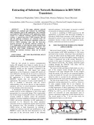
Goal<br />
C 1 C 2 C 3 C 4<br />
A 1 A 2 A 3<br />
Fig. 1. A simple AHP model.<br />
AHP is one of the most popular MCDM tools <strong>for</strong> <strong>for</strong>mulat<strong>in</strong>g <strong>and</strong> analyz<strong>in</strong>g decisions. The technique<br />
is employed <strong>for</strong> rank<strong>in</strong>g a set of alternatives or <strong>for</strong> the selection of the best <strong>in</strong> a set of alternatives. The<br />
rank<strong>in</strong>g/selection is done with respect to an overall goal, which is broken down <strong>in</strong>to a set of criteria. A<br />
brief discussion of AHP is provided <strong>in</strong> this section. More detailed description of AHP <strong>and</strong> application<br />
issues can be found <strong>in</strong> Saaty [13]. AHP has been applied to numerous practical problems <strong>in</strong> the last few<br />
decades [21].<br />
Application of AHP to a decision problem <strong>in</strong>volves four steps [22].<br />
Step 1: Structur<strong>in</strong>g of the decision problem <strong>in</strong>to a hierarchical model. It <strong>in</strong>cludes decomposition of<br />
the decision problem <strong>in</strong>to elements accord<strong>in</strong>g to their common characteristics <strong>and</strong> the <strong>for</strong>mation of a<br />
hierarchical model hav<strong>in</strong>g different levels. A simple AHP model (Fig. 1) has three levels (goal, criteria<br />
<strong>and</strong> alternatives). Though the simple model with three levels shown <strong>in</strong> Fig. 1 is the most common AHP<br />
model, more complex models conta<strong>in</strong><strong>in</strong>g more than three levels are also used <strong>in</strong> the literature. For example,<br />
criteria can be divided further <strong>in</strong>to sub-criteria <strong>and</strong> sub-sub-criteria. Additional levels conta<strong>in</strong><strong>in</strong>g different<br />
actors relevant to the problem under consideration may also be <strong>in</strong>cluded <strong>in</strong> AHP studies [13].<br />
Step 2: Mak<strong>in</strong>g pair-wise comparisons <strong>and</strong> obta<strong>in</strong><strong>in</strong>g the judgment matrix. In this step, the elements<br />
of a particular level are compared with respect to a specific element <strong>in</strong> the immediate upper level. The<br />
result<strong>in</strong>g <strong>weight</strong>s of the elements may be called the local <strong>weight</strong>s (to be contrasted with f<strong>in</strong>al <strong>weight</strong>s,<br />
discussed <strong>in</strong> Step 4).<br />
The op<strong>in</strong>ion of a decision-maker (DM) is elicited <strong>for</strong> compar<strong>in</strong>g the elements. Elements are compared<br />
pair-wise <strong>and</strong> judgments on comparative attractiveness of elements are captured us<strong>in</strong>g a rat<strong>in</strong>g scale (1–9<br />
scale <strong>in</strong> traditional AHP [13]). Usually, an element receiv<strong>in</strong>g higher rat<strong>in</strong>g is viewed as superior (or more<br />
attractive) compared to another one that receives a lower rat<strong>in</strong>g. The comparisons are used to <strong>for</strong>m a<br />
matrix of pair-wise comparisons called the judgment matrix A. Each entry aij of the judgment matrix are<br />
governed by the three rules: aij > 0; aij =1/aji; <strong>and</strong> aii =1 <strong>for</strong> all i. If the transitivity property holds, i.e.,<br />
aij = aik ∗ akj , <strong>for</strong> all the entries of the matrix, then the matrix is said to be consistent. If the property does<br />
not hold <strong>for</strong> all the entries, the level of <strong>in</strong>consistency can be captured by a measure called consistency<br />
ratio [13] (see next step).<br />
For the model shown <strong>in</strong> Fig. 1, five judgment matrices need to be elicited from DM—one <strong>for</strong> estimat<strong>in</strong>g<br />
the local <strong>weight</strong>s of criteria with respect to the goal (see Table 2A <strong>for</strong> an illustrative judgment matrix), <strong>and</strong><br />
one each <strong>for</strong> comput<strong>in</strong>g the local <strong>weight</strong>s of alternatives with respect to each of the four criteria (Table<br />
2B–E). All the entries <strong>in</strong> Table 2A–E, except the local <strong>weight</strong>s, are hypothetical values.
R. Ramanathan / Computers & Operations Research 33 (2006) 1289–1307 1293<br />
Table 2<br />
Illustration of AHP calculations <strong>for</strong> the model shown <strong>in</strong> Fig. 1<br />
A: Comparison of criteria with respect to goal<br />
C1 C2 C3 C4 Local <strong>weight</strong>s<br />
C1 1 1 4 5 0.400<br />
C2 1 1 5 3 0.394<br />
C3 1/4 1/5 1 3 0.128<br />
C4 1/5 1/3 1/3 1 0.078<br />
Consistency ratio = 0.088<br />
B: Comparison of alternatives with respect to C1<br />
A1 A2 A3 Local <strong>weight</strong>s<br />
A1 1 1/3 5 0.279<br />
A2 3 1 7 0.649<br />
A3 1/5 1/7 1 0.072<br />
Consistency ratio = 0.055<br />
C: Comparison of alternatives with respect to C2<br />
A1 A2 A3 Local <strong>weight</strong>s<br />
A1 1 1/9 1/5 0.060<br />
A2 9 1 4 0.709<br />
A3 5 1/4 1 0.231<br />
Consistency ratio = 0.061<br />
D: Comparison of alternatives with respect to C3<br />
A1 A2 A3 Local <strong>weight</strong>s<br />
A1 1 2 5 0.582<br />
A2 1/2 1 3 0.309<br />
A3 1/5 1/3 1 0.109<br />
Consistency ratio = 0.003<br />
E: Comparison of alternatives with respect to C4<br />
A1 A2 A3 Local <strong>weight</strong>s<br />
A1 1 3 9 0.692<br />
A2 1/3 1 3 0.231<br />
A3 1/9 1/3 1 0.077<br />
Consistency ratio = 0.000<br />
F: F<strong>in</strong>al <strong>weight</strong>s of alternatives<br />
A1<br />
A2<br />
A3<br />
0.261<br />
0.590<br />
0.148
1294 R. Ramanathan / Computers & Operations Research 33 (2006) 1289–1307<br />
Step 3: Local <strong>weight</strong>s <strong>and</strong> consistency of comparisons. In this step, local <strong>weight</strong>s of the elements are<br />
calculated from the judgment matrices us<strong>in</strong>g the eigenvector method (EVM). The normalized eigenvector<br />
correspond<strong>in</strong>g to the pr<strong>in</strong>cipal eigenvalue of the judgment matrix provides the <strong>weight</strong>s of the correspond<strong>in</strong>g<br />
elements. Though EVM is followed widely <strong>in</strong> traditional AHP computations, other methods are also<br />
suggested <strong>for</strong> calculat<strong>in</strong>g <strong>weight</strong>s, <strong>in</strong>clud<strong>in</strong>g the logarithmic least-square technique (LLST) [23,24], goal<br />
programm<strong>in</strong>g [25], <strong>and</strong> others [26]. When EVM is used, consistency ratio (CR) can be computed. For a<br />
consistent matrix CR = 0. A value of CR less than 0.1 is considered acceptable because human judgments<br />
need not be always consistent, <strong>and</strong> there may be <strong>in</strong>consistencies <strong>in</strong>troduced because of the nature of scale<br />
used. If CR <strong>for</strong> a matrix is more than 0.1, judgments should be elicited once aga<strong>in</strong> from the DM till he<br />
gives more consistent judgments. Local <strong>weight</strong>s computed <strong>for</strong> the illustrative judgment matrices us<strong>in</strong>g<br />
EVM <strong>and</strong> the correspond<strong>in</strong>g CR values are also shown <strong>in</strong> Table 2A–E.<br />
Step 4: Aggregation of <strong>weight</strong>s across various levels to obta<strong>in</strong> the f<strong>in</strong>al <strong>weight</strong>s of alternatives. Once<br />
the local <strong>weight</strong>s of elements of different levels are obta<strong>in</strong>ed as outl<strong>in</strong>ed <strong>in</strong> Step 3, they are aggregated<br />
to obta<strong>in</strong> f<strong>in</strong>al <strong>weight</strong>s of the decision alternatives (elements at the lowest level). For example, the f<strong>in</strong>al<br />
<strong>weight</strong> of alternative A1 is computed us<strong>in</strong>g the follow<strong>in</strong>g hierarchical (arithmetic) <strong>aggregation</strong> rule <strong>in</strong><br />
traditional AHP:<br />
F<strong>in</strong>al <strong>weight</strong> of A1 = <br />
<br />
Local <strong>weight</strong> of A1 with Local <strong>weight</strong> of<br />
×<br />
. (5)<br />
respect of criterion Cj criterion Cj<br />
j<br />
By def<strong>in</strong>ition, the <strong>weight</strong>s of alternatives <strong>and</strong> importance of criteria are normalized so that they sum to<br />
unity.<br />
Note that a geometric variant of the above <strong>aggregation</strong> rule can also be used, especially when LLST<br />
is used <strong>for</strong> comput<strong>in</strong>g local <strong>weight</strong>s [24]. The f<strong>in</strong>al <strong>weight</strong>s represent the rat<strong>in</strong>g of the alternatives <strong>in</strong><br />
achiev<strong>in</strong>g the goal of the problem.<br />
The f<strong>in</strong>al <strong>weight</strong>s computed us<strong>in</strong>g (5) <strong>for</strong> the illustration are shown <strong>in</strong> Table 2F. Thus, given the<br />
hypothetical judgments of Table 2A–E, alternative A2 is the most preferred alternative, followed by<br />
alternatives A1 <strong>and</strong> then A3.<br />
The popularity of AHP stems from its simplicity, flexibility, <strong>in</strong>tuitive appeal <strong>and</strong> its ability to mix<br />
quantitative <strong>and</strong> qualitative criteria <strong>in</strong> the same decision framework. Despite its popularity, some shortcom<strong>in</strong>gs<br />
of AHP have been reported <strong>in</strong> the literature, which have limited its applicability. The number<br />
of judgements to be elicited <strong>in</strong> AHP <strong>in</strong>creases as the number of alternatives <strong>and</strong> criteria <strong>in</strong>crease. This is<br />
often a tiresome <strong>and</strong> exert<strong>in</strong>g exercise <strong>for</strong> the DM. The issue of rank reversal [27] is one of the prom<strong>in</strong>ent<br />
limitations of traditional AHP. The rank<strong>in</strong>g of alternatives determ<strong>in</strong>ed by the traditional AHP may be<br />
altered by the addition or deletion of another alternative <strong>for</strong> consideration. For example, when a new<br />
alternative A4 is added to the list of alternatives discussed earlier, or when an exist<strong>in</strong>g alternative A1, A2<br />
orA3 is removed, it is possible that their rank<strong>in</strong>gs change. Modifications to the traditional AHP have been<br />
suggested [24] to avoid the problem of rank reversal.<br />
2.3. A literature survey on l<strong>in</strong>k<strong>in</strong>g DEA <strong>and</strong> AHP<br />
Both DEA <strong>and</strong> AHP are versatile tools <strong>in</strong> their own fields. While DEA has traditionally found applications<br />
<strong>for</strong> per<strong>for</strong>mance measurement of DMUs, AHP has been widely applied <strong>in</strong> MCDM problems<br />
<strong>for</strong> estimat<strong>in</strong>g <strong>weight</strong>s of alternatives when several criteria, both qualitative <strong>and</strong> quantitative, have to be<br />
considered. In fact, many modern complex issues have been tackled us<strong>in</strong>g a comb<strong>in</strong>ation of both the
R. Ramanathan / Computers & Operations Research 33 (2006) 1289–1307 1295<br />
methods. Some articles have used AHP <strong>for</strong> h<strong>and</strong>l<strong>in</strong>g subjective factors <strong>and</strong> to generate a set of numerical<br />
values, <strong>and</strong> then used DEA to identify efficiency score based on the entire data, <strong>in</strong>clud<strong>in</strong>g those generated<br />
by the AHP [28,29]. S<strong>in</strong>uany-Stern et al. [30] have applied DEA on pairs of units, used the result<strong>in</strong>g DEA<br />
scores to generate a pair-wise comparison matrix <strong>and</strong> then applied AHP to generate <strong>weight</strong>s of units from<br />
the matrix.<br />
AHP has also been used to <strong>in</strong>troduce preference <strong>in</strong><strong>for</strong>mation <strong>in</strong> DEA calculations. Preference <strong>in</strong><strong>for</strong>mation<br />
is <strong>in</strong>troduced <strong>in</strong> the <strong>for</strong>m of subjective <strong>weight</strong>s derived us<strong>in</strong>g AHP [31,32]. Both these studies have<br />
<strong>in</strong>corporated AHP <strong>weight</strong>s <strong>in</strong> DEA us<strong>in</strong>g the method of assurance region [33].<br />
Some papers have applied both the methods <strong>for</strong> a given problem <strong>and</strong> compared their outputs [34–36].<br />
In addition, DEA <strong>and</strong> AHP have been l<strong>in</strong>ked with other techniques <strong>for</strong> specific applications (e.g., DEA<br />
with discrim<strong>in</strong>ant <strong>analysis</strong> <strong>and</strong> goal programm<strong>in</strong>g [37], AHP with goal programm<strong>in</strong>g [38], <strong>and</strong> AHP<br />
with compromise programm<strong>in</strong>g [39]). In this paper, the concepts of efficiency measurement <strong>in</strong> DEA are<br />
<strong>in</strong>tegrated with the concepts of <strong>weight</strong> measurement <strong>in</strong> AHP.<br />
3. A synthesis of concepts of DEA <strong>in</strong> deriv<strong>in</strong>g <strong>weight</strong>s <strong>in</strong> AHP<br />
In this section, it is proposed that DEA concepts can be used <strong>in</strong> the last two steps of apply<strong>in</strong>g AHP to a<br />
decision problem—namely, deriv<strong>in</strong>g local <strong>weight</strong>s from a given judgment matrix (Step 3) <strong>and</strong> aggregat<strong>in</strong>g<br />
local <strong>weight</strong>s to get f<strong>in</strong>al <strong>weight</strong>s (Step 4).<br />
3.1. Us<strong>in</strong>g DEA concepts <strong>for</strong> deriv<strong>in</strong>g local <strong>weight</strong>s from a judgment matrix<br />
In this section, we propose DEA <strong>for</strong> deriv<strong>in</strong>g local <strong>weight</strong>s from a judgment matrix. Efficiency calculations<br />
us<strong>in</strong>g DEA require outputs <strong>and</strong> <strong>in</strong>puts. Each row of the judgment matrix is viewed as a DMU <strong>and</strong><br />
each column of the judgement matrix is viewed as an output. Thus a judgement matrix of size n × n will<br />
have n DMUs <strong>and</strong> n outputs. Note that the entries of the matrix are viewed as outputs as they have the<br />
characteristics of outputs, viz. an element hav<strong>in</strong>g higher rat<strong>in</strong>g is viewed better than the one that has a<br />
lower rat<strong>in</strong>g. S<strong>in</strong>ce DEA calculations cannot be made entirely with outputs <strong>and</strong> require at least one <strong>in</strong>put,<br />
a dummy <strong>in</strong>put that has a value of 1 <strong>for</strong> all the DMUs is employed. A comparison of traditional AHP<br />
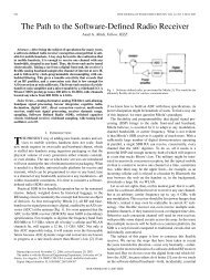
view <strong>and</strong> the proposed DEA view of a judgement matrix is shown <strong>in</strong> Fig. 2. It is proposed <strong>in</strong> this paper<br />
that the efficiency scores calculated us<strong>in</strong>g DEA models such as Models 1–4 could be <strong>in</strong>terpreted as the<br />
local <strong>weight</strong>s of the DMUs.<br />
3.1.1. Local <strong>weight</strong>s us<strong>in</strong>g DEA <strong>for</strong> consistent judgment matrices<br />
When applied to a consistent matrix, <strong>for</strong> which <strong>weight</strong>s are known, DEA correctly estimates the true<br />
<strong>weight</strong>s. Specifically, suppose that a predeterm<strong>in</strong>ed set of n <strong>weight</strong>s, say w1,w2,...,wn, is used to create<br />
a consistent judgment matrix of size n given by<br />
⎡<br />
w1/w1 w1/w2 ···<br />
⎤<br />
w1/wn<br />
⎢ w2/w1<br />
W = ⎢<br />
⎣<br />
.<br />
w2/w2<br />
.<br />
···<br />
.<br />
w2/wn ⎥<br />
.<br />
⎦<br />
wn/w1 wn/w2 ··· wn/wn<br />
.
1296 R. Ramanathan / Computers & Operations Research 33 (2006) 1289–1307<br />
Element 1<br />
Traditional AHP View Proposed DEA View<br />
Element 2<br />
…<br />
Element n<br />
Element 1 1 a 12 … a 1N<br />
Element 2 1/ a 12 1 … a 2N<br />
… … … … …<br />
Element N 1/ a 1 N 1/ a 2 N … 1<br />
Output 1<br />
Output 2<br />
…<br />
Output n<br />
DMU 1 1 a 12 … a 1N<br />
DMU 2 1/ a 12 1 … a 2N 1<br />
Dummy <strong>in</strong>put<br />
… … … … … …<br />
DMU N 1/ a 1N 1/ a 2 N … 1 1<br />
Fig. 2. A comparison of the traditional AHP view <strong>and</strong> the proposed DEA view of a judgement matrix.<br />
Any <strong>weight</strong> <strong>derivation</strong> method, when applied to the above matrix W, should generate the true <strong>weight</strong>s<br />
w1,w2,...,wn. DEA correctly calculates the true <strong>weight</strong>s <strong>for</strong> a consistent judgment matrix as proved <strong>in</strong><br />
Theorem 1. Note that it is not possible to make a similar verification <strong>for</strong> <strong>in</strong>consistent matrices, because<br />
there is no unique correct answer.<br />
Theorem 1. For a consistent judgment matrix, the local <strong>weight</strong>s of alternatives computed us<strong>in</strong>g DEA<br />
co<strong>in</strong>cide with the correct <strong>weight</strong>s used to <strong>for</strong>m the matrix.<br />
Proof. Let there be n elements <strong>for</strong> comparison, lead<strong>in</strong>g to a judgment matrix W of size n. Without loss<br />
of generality, assume that w1 w2 ···wn where wi represents the true <strong>weight</strong> of element i.<br />
Model 4, with one dummy constant <strong>in</strong>put, <strong>for</strong> comput<strong>in</strong>g the <strong>weight</strong> of element m is the follow<strong>in</strong>g:<br />
Model 6<br />
max m<br />
such that<br />
n wi<br />
k mi, i=1 wm<br />
n<br />
mi 1,<br />
i=1<br />
0; m free,<br />
where are the multipliers. Subscript m represents the element <strong>for</strong> which the efficiency is be<strong>in</strong>g computed.<br />
Note that, because of the nature of the consistent judgment matrix, the set of constra<strong>in</strong>ts Y mYm <strong>in</strong><br />
Model 4 reduces to a s<strong>in</strong>gle constra<strong>in</strong>t m n i=1 (wi/wm)mi <strong>in</strong> Model 6. Aga<strong>in</strong> because of the presence<br />
of s<strong>in</strong>gle constant dummy <strong>in</strong>put, the second set of constra<strong>in</strong>ts XXm <strong>in</strong> Model 4 reduces to a s<strong>in</strong>gle<br />
constra<strong>in</strong>t n i=1mi 1 <strong>in</strong> Model 6. Further, it has been proved that this constra<strong>in</strong>t reduces to strict equality<br />
ni=1<br />
mi = 1 at the optimal solution [40].<br />
Substitute m = n <strong>in</strong> Model 6 to compute the <strong>weight</strong> of the last element n. At the optimal solution,<br />
∗ nn = 1 − n−1 i=1 ∗ where asterisk <strong>in</strong>dicates optimal solution. Substitut<strong>in</strong>g <strong>in</strong> the first constra<strong>in</strong>t of<br />
ni<br />
1<br />
(6)
R. Ramanathan / Computers & Operations Research 33 (2006) 1289–1307 1297<br />
Table 3<br />
A look at the entries of Table 2A from the DEA perspective<br />
DMU Output 1 Output 2 Output 3 Output 4 Input (dummy) DEA efficiency<br />
C1 1 1 4 5 1 1<br />
C2 1 1 5 3 1 1<br />
C3 1/4 1/5 1 3 1 0.6<br />
C4 1/5 1/3 1/3 1 1 0.333<br />
Model 6, we get<br />
⎧<br />
∗ n <br />
w1<br />
wn<br />
⎪⎨<br />
∗ w2<br />
n1 + wn ∗ wn−1<br />
n2 +···+ wn ∗ n,n−1<br />
w1<br />
wn ∗ w2<br />
n1 + wn ∗ wn−1<br />
n2 +···+ wn ∗ n,n−1 +<br />
⎪⎩<br />
+ wn<br />
wn ∗ nn ,<br />
<br />
w1 1 + − 1 wn ∗ n1 +<br />
<br />
w2 − 1 wn ∗ n2 +···+<br />
<br />
1 − n−1 <br />
<br />
,<br />
<br />
i=1<br />
∗ ni<br />
<br />
wn−1 − 1 wn ∗ n,n−1 .<br />
If w1 w2 ···wn, all the entries <strong>in</strong> square brackets <strong>in</strong> the last equation of (7) will be negative. Hence,<br />
the maximum value of ∗ n occurs when all the ∗ are at their m<strong>in</strong>imum, i.e., when ∗ n1 =∗ n2 =···=∗ n,n−1 =0.<br />
Hence the optimal solution is ∗ n = 1, ∗ nn = 1 <strong>and</strong> ∗ = 0, i = 1, 2,...,n− 1.<br />
ni<br />
Us<strong>in</strong>g a similar logic, it can be proved that ∗ 1 = wn/w1, ∗ 2 = wn/w2,..., ∗ n−1 = wn/wn−1. Due<br />
to the nature of the output-oriented <strong>envelopment</strong> DEA <strong>for</strong>mulation, <strong>weight</strong>s are actually the reciprocals<br />
of . Thus, the <strong>weight</strong>s of the elements are <strong>in</strong> the ratio [w1/wn,w2/wn,...,wn−1/wn, 1] or<br />
[w1,w2,...,wn−1]. <br />
3.1.2. Numerical illustration<br />
As an example, consider Table 2A, which is a judgment matrix <strong>for</strong> compar<strong>in</strong>g criteria with respect to<br />
the goal. In the proposed approach, the entries of Table 2A are viewed as the per<strong>for</strong>mance (row-wise) of<br />
DMUs C1, C2, C3 <strong>and</strong> C4 <strong>in</strong> terms of four outputs. The output–<strong>in</strong>put structure of DEA is shown <strong>in</strong> Table<br />
3. In this case, any of Models 1–4 can be applied to get the local <strong>weight</strong>s of the criteria. For example, to<br />
get the f<strong>in</strong>al <strong>weight</strong> of criterion C1, the follow<strong>in</strong>g model (based on Model 1) can be used:<br />
Model 8<br />
max z = v11 + v12 + 4v13 + 5v14<br />
s.t. u11 = 1,<br />
v11 + v12 + 4v13 + 5v14 − u11 0,<br />
v11 + v12 + 5v13 + 3v14 − u11 0,<br />
1/4v11 + 1/5v12 + v13 + 3v14 − u11 0,<br />
1/5v11 + 1/3v12 + 1/3v13 + v14 − u11 0,<br />
v11,v12,v13,v14,u11 0.<br />
(7)<br />
(8)
1298 R. Ramanathan / Computers & Operations Research 33 (2006) 1289–1307<br />
Traditional AHP View Proposed DEA View<br />
Criterion 1<br />
Criterion 2<br />
…<br />
Alternative 1 y 11 y 12 … y 1J<br />
Alternative 2 y 21 y 22 … y 2J<br />
Criterion J<br />
… … … … …<br />
Alternative N y N1 y N2 … y NJ<br />
Output 1<br />
Output 2<br />
…<br />
Output J<br />
DMU 1 y 11 y 12 … y 1J 1<br />
DMU 2 y 21 y 22 … y 2J 1<br />
… … … … … …<br />
DMU N y N1 y N2 … y NJ 1<br />
Fig. 3. A comparison of the traditional AHP view <strong>and</strong> the proposed DEA view of the matrix of local <strong>weight</strong>s of alternatives with<br />
respect to all criteria.<br />
In the above model, the first subscript (i.e., 1) refers to the reference DMU <strong>for</strong> which efficiency is<br />
be<strong>in</strong>g computed (criterion C1 here). The optimal objective function value of Model 8, when solved, will<br />
give the local <strong>weight</strong> of criterion C1. To get the f<strong>in</strong>al <strong>weight</strong> of other criteria, models similar to Model 8<br />
should be solved by chang<strong>in</strong>g the objective function. The DEA efficiency scores represent<strong>in</strong>g the local<br />
<strong>weight</strong>s of DMUs (i.e., the criteria here) are presented <strong>in</strong> the last column of Table 3 (1.000, 1.000, 0.600,<br />
<strong>and</strong> 0.333).<br />
Weights computed us<strong>in</strong>g the DEA approach differs from those obta<strong>in</strong>ed us<strong>in</strong>g EVM (see Table 2A).<br />
Note that, <strong>for</strong> compar<strong>in</strong>g with the <strong>weight</strong>s computed by DEA, the local <strong>weight</strong>s obta<strong>in</strong>ed us<strong>in</strong>g EVM<br />
should be adjusted by divid<strong>in</strong>g all the <strong>weight</strong>s by the largest one, result<strong>in</strong>g <strong>in</strong> the <strong>weight</strong>s 1, 0.985, 0.319,<br />
<strong>and</strong> 0.195. These <strong>weight</strong>s are different from those calculated by DEA (last column of Table 3). The<br />
difference is because of the assumptions underly<strong>in</strong>g the methods.<br />
Note that while DMU C1 “produces” more Output 4, DMU C2 “produces” more Output 3 <strong>and</strong> hence it<br />
is not possible to say which one is better than the other. However, DMUs C1 <strong>and</strong> C2 have produced more<br />
or equal amounts of outputs compared to DMU C3 while all the DMUs produced more or equal amounts<br />
of outputs compared to DMU C4. It is not possible to conclusively say that the DM prefers C1 or C2,but<br />
it is possible to conclusively say that he prefers C1 <strong>and</strong> C2 to C3, <strong>and</strong>, C1, C2 <strong>and</strong> C3 to C4. This leads<br />
to a situation to believe that the DM would rank C1 <strong>and</strong> C2 at the same level, then rank C3 <strong>and</strong> rank C4<br />
at the bottom. Thus DEA assigns <strong>in</strong> unit efficiency scores <strong>for</strong> C1 <strong>and</strong> C2, a lower score <strong>for</strong> C3 (0.6) <strong>and</strong><br />
the lowest score <strong>for</strong> C4 (0.333).<br />
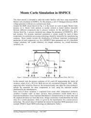
3.2. Aggregation of local <strong>weight</strong>s to get f<strong>in</strong>al <strong>weight</strong>s<br />
In this section, we propose DEA to aggregate local <strong>weight</strong>s to get f<strong>in</strong>al <strong>weight</strong>s of elements (Step 4 of<br />
AHP). Suppose the local <strong>weight</strong>s of alternatives <strong>in</strong> terms of all the criteria are available as shown <strong>in</strong> Fig.<br />
3. The entry ymj represents the local <strong>weight</strong> of alternative m with respect to criterion j. In traditional AHP,<br />
the arithmetic <strong>aggregation</strong> rule (5) is employed <strong>for</strong> <strong>aggregation</strong>. DEA is proposed <strong>in</strong> this paper <strong>for</strong> the<br />
<strong>aggregation</strong>. When DEA is used, alternatives are considered as DMUs <strong>and</strong> their local <strong>weight</strong>s <strong>in</strong> terms of<br />
Dummy <strong>in</strong>put
R. Ramanathan / Computers & Operations Research 33 (2006) 1289–1307 1299<br />
the criteria will be viewed as outputs. With a dummy <strong>in</strong>put, the DEA view of the matrix of local <strong>weight</strong>s<br />
is also shown <strong>in</strong> Fig. 3.<br />
Normally, when local <strong>weight</strong>s are aggregated to f<strong>in</strong>al <strong>weight</strong>s, the importance measures of criteria<br />
(local <strong>weight</strong>s of criteria <strong>in</strong> this case) are also used. For example, the <strong>aggregation</strong> rule (5) is <strong>weight</strong>ed<br />
arithmetic <strong>aggregation</strong> <strong>in</strong>corporat<strong>in</strong>g the local <strong>weight</strong>s of <strong>weight</strong>s. However, DEA does not normally<br />
require the local <strong>weight</strong>s of criteria <strong>for</strong> <strong>aggregation</strong>. Hence, <strong>aggregation</strong> us<strong>in</strong>g DEA could be discussed<br />
under two cases: (a) without consider<strong>in</strong>g the local <strong>weight</strong>s of criteria <strong>for</strong> <strong>aggregation</strong> <strong>and</strong> (b) consider<strong>in</strong>g<br />
local <strong>weight</strong>s of criteria.<br />
Case (a): When DEA is used <strong>for</strong> <strong>aggregation</strong>, the importance measures of criteria are automatically<br />
generated by DEA as the values of multipliers us<strong>in</strong>g l<strong>in</strong>ear programm<strong>in</strong>g. In this case, a simple DEA<br />
model (any of models 1–4) of data <strong>in</strong> Fig. 3 could be used to get the f<strong>in</strong>al <strong>weight</strong>s of alternatives. Hence,<br />
the local <strong>weight</strong>s of criteria are not necessary <strong>in</strong> DEA.<br />
Case (b): If needed, the importance measures of criteria can be imposed <strong>in</strong> DEA us<strong>in</strong>g the method of<br />
assurance region [33]. This is done by append<strong>in</strong>g additional constra<strong>in</strong>ts that specify relationships among<br />
the multipliers <strong>in</strong> the orig<strong>in</strong>al DEA model. For example, the importance of criteria are <strong>in</strong>corporated <strong>in</strong><br />
Model 1 <strong>in</strong> the <strong>for</strong>m of multipliers vm1 = dj vmj (<strong>for</strong> all j = 1, 2,...,J <strong>and</strong> d1 = 1). If criterion 1 is half<br />
<strong>and</strong> thrice as important as criteria 2 <strong>and</strong> 3, respectively, then d2 = 1/2 <strong>and</strong> d3 = 3. An <strong>in</strong>terest<strong>in</strong>g theorem<br />
<strong>for</strong> this Case (b) is proved <strong>in</strong> the next section.<br />
The above <strong>aggregation</strong> procedures assume a simple AHP model. The procedures could be extended<br />
<strong>for</strong> more complex models hav<strong>in</strong>g more levels, but we consider the simple model <strong>in</strong> the rema<strong>in</strong>der of this<br />
section.<br />
3.2.1. Aggregation to f<strong>in</strong>al <strong>weight</strong>s us<strong>in</strong>g DEA when relationships among importance of criteria are<br />
exogenously specified<br />
When the importance of criteria are exogenously specified <strong>and</strong> <strong>in</strong>corporated <strong>in</strong> a DEA model by<br />
provid<strong>in</strong>g additional constra<strong>in</strong>ts restrict<strong>in</strong>g the values of multipliers as <strong>in</strong> Case (b) above, the f<strong>in</strong>al <strong>weight</strong>s<br />
of alternatives estimated by DEA is proportional to the <strong>weight</strong>ed sum of local <strong>weight</strong>s as shown <strong>in</strong> Theorem<br />
2.<br />
Theorem 2. Let the local <strong>weight</strong>s of alternatives with respect to different criteria be given by<br />
⎡<br />
⎢<br />
⎣<br />
.<br />
y11 y12 ··· y1J<br />
y21 y22 ··· y2J<br />
. ···<br />
yN1 yN2 ··· yNJ<br />
.<br />
⎤<br />
⎥<br />
⎦ ,<br />
where ymj is the local <strong>weight</strong> of alternative m with respect to criterion j. There are N alternatives <strong>and</strong><br />
J criteria. If the importance of criteria are <strong>in</strong>corporated <strong>in</strong> the <strong>for</strong>m of multipliers vm1 = dj vmj (<strong>for</strong> all<br />
j = 1, 2,...,J <strong>and</strong> d1 = 1) then f<strong>in</strong>al <strong>weight</strong>s aggregated us<strong>in</strong>g DEA is proportional to the <strong>weight</strong>ed sum<br />
Jj=1 dj ymj <strong>for</strong> alternative m.<br />
Proof. We use the <strong>for</strong>mulation shown by Model 1 <strong>for</strong> the proof here. For comput<strong>in</strong>g the f<strong>in</strong>al <strong>weight</strong> of<br />
the alternative m Model 1 can be written as follows:
1300 R. Ramanathan / Computers & Operations Research 33 (2006) 1289–1307<br />
Model 9<br />
max<br />
subject to<br />
J<br />
vmj ymj<br />
j=1<br />
um1 = 1;<br />
J<br />
vmj ynj − um1 0; n = 1, 2,...,N,<br />
j=1<br />
vmj ,um1 0; j = 1, 2,...,J.<br />
When the importance of criteria are <strong>in</strong>corporated by <strong>in</strong>troduc<strong>in</strong>g additional constra<strong>in</strong>ts of the <strong>for</strong>m<br />
vm1 = dj vmj (<strong>for</strong> all j = 1, 2,...,J <strong>and</strong> d1 = 1) <strong>in</strong> Model 9, the model can be rewritten as follows:<br />
Model 10<br />
max vm1<br />
s.t.<br />
J<br />
dj ymj<br />
j=1<br />
J<br />
vm1<br />
j=1<br />
vn1 0.<br />
dj ynj 1; n = 1, 2,...,N,<br />
Jj=1 Model 10 will choose the value of vm1 such that the largest value of the constra<strong>in</strong>ts vm1 dj ynj is<br />
equal to unity <strong>for</strong> n = 1, 2,...,N. S<strong>in</strong>ce these constra<strong>in</strong>ts are the same <strong>for</strong> all the N DEA <strong>for</strong>mulations<br />
<strong>for</strong> f<strong>in</strong>d<strong>in</strong>g the efficiency of all the N DMUs, the value of vm1 is the same <strong>for</strong> all the DEA programs. Thus,<br />
the efficiency score of the mth DMU is proportional to J j=1dj ymj .<br />
Corollary 1. If all the criteria have equal <strong>weight</strong>s, then the f<strong>in</strong>al <strong>weight</strong>s are proportional simple sum<br />
Jj=1 ymj .<br />
Proof. If all the criteria have equal <strong>weight</strong>s, the multipliers have equal value. In this case, dj = 1 <strong>for</strong> all<br />
j = 1, 2,...,J. Hence the efficiency score of the mth DMU is proportional to J j=1 dj ymj or J j=1 ymj .<br />
<br />
3.2.2. Numerical illustration<br />
The calculations of the proposed approach can be illustrated us<strong>in</strong>g the entries of Table 2B–E. The local<br />
<strong>weight</strong>s of alternatives with respect to each of the criteria can be computed us<strong>in</strong>g DEA as expla<strong>in</strong>ed <strong>in</strong><br />
Section 3.1. The local <strong>weight</strong>s are shown <strong>in</strong> Table 4 (columns 2–5). Aggregation us<strong>in</strong>g DEA is discussed<br />
below <strong>for</strong> the two cases, (a) <strong>and</strong> (b).<br />
Case (a): Without us<strong>in</strong>g the local <strong>weight</strong>s of criteria: In this case, any of the models (1) to (4) are<br />
applied <strong>for</strong> the local <strong>weight</strong>s <strong>in</strong> Table 4. The local <strong>weight</strong>s are considered as outputs of alternatives, <strong>and</strong><br />
(9)<br />
(10)
R. Ramanathan / Computers & Operations Research 33 (2006) 1289–1307 1301<br />
Table 4<br />
Local <strong>and</strong> f<strong>in</strong>al <strong>weight</strong>s of alternatives computed us<strong>in</strong>g the proposed approach<br />
Local <strong>weight</strong>s of alternatives with F<strong>in</strong>al <strong>weight</strong>s<br />
respect to <strong>in</strong>dividual criteria<br />
C1 C2 C3 C4 Case (a) Case (b)<br />
no restrictions with additional restrictions<br />
on criteria vm1 = vm2;<br />
<strong>weight</strong>s vm1 = (1/0.6)vm3; vm1 = 3vm4<br />
A1 0.714 0.111 1.000 1.000 1.000 0.712<br />
A2 1.000 1.000 0.600 0.333 1.000 1.000<br />
A3 0.143 0.556 0.200 0.111 0.556 0.346<br />
a dummy <strong>in</strong>put is <strong>in</strong>troduced. For example, to get the f<strong>in</strong>al <strong>weight</strong> of alternative A1, the follow<strong>in</strong>g model<br />
(based on Model 1) can be used:<br />
Model 11<br />
max z = 0.714v11 + 0.111v12 + v13 + v14<br />
s.t. u11 = 1,<br />
0.714v11 + 0.111v12 + v13 + v14 − u11 0,<br />
v11 + v12 + 0.6v13 + 0.333v14 − u11 0,<br />
0.143v11 + 0.556v12 + 0.2v13 + 0.111v14 − u11 0,<br />
v11,v12,v13,v14,u11 0.<br />
The optimal objective function value of Model 11, when solved, will give the f<strong>in</strong>al <strong>weight</strong> of alternative<br />
A1. To get the f<strong>in</strong>al <strong>weight</strong> of other alternatives, models similar to Model 11 should be solved by chang<strong>in</strong>g<br />
the objective function. The result<strong>in</strong>g f<strong>in</strong>al <strong>weight</strong>s of all the three alternatives are shown <strong>in</strong> Table 4 (1.000,<br />
1.000, <strong>and</strong> 0.556). These <strong>weight</strong>s are logical because A1 per<strong>for</strong>ms well <strong>in</strong> terms of Criteria C3 <strong>and</strong> C4,<br />
while A2 per<strong>for</strong>ms well <strong>in</strong> terms of Criteria C1 <strong>and</strong> C2, <strong>and</strong> hence it is not possible to decide which one<br />
of them is better.<br />
Case (b): us<strong>in</strong>g the local <strong>weight</strong>s of criteria: In many AHP studies, the importance measures of criteria<br />
are usually considered while calculat<strong>in</strong>g the f<strong>in</strong>al <strong>weight</strong>s. Us<strong>in</strong>g the values of local <strong>weight</strong>s of criteria<br />
(see Table 3), the follow<strong>in</strong>g additional constra<strong>in</strong>ts can be <strong>in</strong>troduced <strong>in</strong> the DEA model that calculates the<br />
f<strong>in</strong>al <strong>weight</strong> of DMU m: vm1 = vm2; vm1 = (1/0.6)vm3; vm1 = 3vm4 . Specifically, when calculat<strong>in</strong>g the<br />
f<strong>in</strong>al <strong>weight</strong> of alternative A1, the follow<strong>in</strong>g constra<strong>in</strong>ts should be added to Model 11: v11 = v12; v11 =<br />
(1/0.6)v13; v11 = 3v14. The result<strong>in</strong>g f<strong>in</strong>al <strong>weight</strong>s of alternatives, shown <strong>in</strong> the last column of Table 4,<br />
are 0.712, 1.000, <strong>and</strong> 0.346. As proved <strong>in</strong> Theorem 2, the f<strong>in</strong>al <strong>weight</strong>s are proportional to the <strong>weight</strong>ed<br />
sum of local <strong>weight</strong>s. For example, <strong>for</strong> alternative A1, the <strong>weight</strong>ed sum can be calculated as [(0.714 ∗<br />
1) + (0.111 ∗ 1) + (1 ∗ 0.6) + (1 ∗ 0.333)] =1.7583. The <strong>weight</strong>ed sum <strong>for</strong> the three alternatives are<br />
1.7583, 2.471, <strong>and</strong> 0.856, which are proportional to 0.712, 1.000, <strong>and</strong> 0.346.<br />
These <strong>weight</strong>s aga<strong>in</strong> seem logical when compared with the <strong>weight</strong>s obta<strong>in</strong>ed us<strong>in</strong>g DEA with no<br />
restrictions on criteria <strong>weight</strong>s. When criteria 3 <strong>and</strong> 4 are given lower importance, alternative A1 which<br />
per<strong>for</strong>ms well <strong>in</strong> terms of these two criteria, cannot be regarded as efficient as alternative A2. Hence, the<br />
DEA scores now result <strong>in</strong> lower <strong>weight</strong> <strong>for</strong> alternative A1.<br />
(11)
1302 R. Ramanathan / Computers & Operations Research 33 (2006) 1289–1307<br />
It is suggested that Case (a) should be preferred when calculat<strong>in</strong>g f<strong>in</strong>al <strong>weight</strong>s of alternatives unless<br />
there is a strong reason to <strong>in</strong>troduce criteria <strong>weight</strong>s (Case (b)). Even if criteria <strong>weight</strong>s are very important,<br />
the f<strong>in</strong>al <strong>weight</strong>s calculated with <strong>and</strong> without restrictions (i.e., Cases (a) <strong>and</strong> (b)) should be presented<br />
together.<br />
Because of the synthesis of concepts of DEA with AHP, the new approach proposed <strong>in</strong> this paper could<br />
be called “data <strong>envelopment</strong> analytic hierarchy process (DEAHP)” (thanks to the common “A” <strong>in</strong> both<br />
the acronyms).<br />
4. Some important characteristics of DEAHP<br />
In this section, some important characteristics of DEAHP are explored <strong>in</strong> more detail.<br />
4.1. Independence of irrelevant alternatives<br />
The rule of <strong>in</strong>dependence of irrelevant alternatives (IIR) can be stated as follows. If an alternative is<br />
elim<strong>in</strong>ated from consideration, then the new order<strong>in</strong>g <strong>for</strong> the rema<strong>in</strong><strong>in</strong>g alternatives should be equivalent<br />
(i.e., same order<strong>in</strong>g) to the orig<strong>in</strong>al order<strong>in</strong>g <strong>for</strong> the same alternatives [41]. This issue of IIR is important<br />
<strong>in</strong> the context of AHP because it has been reported that traditional AHP does not satisfy this rule [27].<br />
DEAHP satisfies this rule as discussed below.<br />
Note that <strong>in</strong> DEAHP, the <strong>weight</strong>s of alternatives (i.e., the efficiency scores) are calculated separately<br />
<strong>for</strong> each alternative us<strong>in</strong>g a separate l<strong>in</strong>ear programm<strong>in</strong>g model. This can be contrasted from the EVM<br />
where <strong>weight</strong>s of all the alternatives are derived simultaneously. In addition, while traditional AHP uses<br />
arithmetic normalization, no such normalization is done <strong>in</strong> the DEAHP. Further, the DEAHP <strong>weight</strong>s are<br />
calculated relative to the <strong>weight</strong> of the best rated alternative.<br />
For the discussion below, efficient alternatives are <strong>in</strong>terpreted as relevant alternatives because they play<br />
an important role <strong>in</strong> the rank order<strong>in</strong>g of all the alternatives. In a general DEA <strong>for</strong>mulation (which is<br />
applicable <strong>for</strong> DEAHP also), if the alternative be<strong>in</strong>g elim<strong>in</strong>ated is not an efficient one (i.e., if the alternative<br />
be<strong>in</strong>g elim<strong>in</strong>ated is an irrelevant alternative), then the new rank<strong>in</strong>g calculated will aga<strong>in</strong> be relative to<br />
the highest ranked one, <strong>and</strong> the order<strong>in</strong>g of alternatives will not change. This is proved <strong>in</strong> Theorem 3<br />
below. For the proof, we use the general DEA <strong>in</strong>put–output matrix shown <strong>in</strong> Table 1. S<strong>in</strong>ce DEAHP is a<br />
particular case of DEA, the results are applicable to DEAHP also.<br />
Theorem 3. Consider the <strong>in</strong>put–output matrix shown <strong>in</strong> Table 1.When DEA is applied to f<strong>in</strong>d the efficiency<br />
scores of the DMUs, the relative rank<strong>in</strong>gs of DMUs will not change if an <strong>in</strong>efficient DMU is removed<br />
from the orig<strong>in</strong>al set of DMUs or added to the orig<strong>in</strong>al set of DMUs.<br />
Proof. We use the DEA <strong>for</strong>mulation given by Model 1 <strong>for</strong> the proof. The model maximizes the objective<br />
function by choos<strong>in</strong>g appropriate values of decision variables V T m , U T m . Note that the objective function<br />
(i.e., the efficiency score) is 1 <strong>for</strong> efficient DMUs <strong>and</strong> less than one <strong>for</strong> <strong>in</strong>efficient DMUs.<br />
Consider the constra<strong>in</strong>ts V T mY − U T mX 0. These represent N constra<strong>in</strong>ts, one each <strong>for</strong> the N DMUs.<br />
First we show that these set of constra<strong>in</strong>ts will not be b<strong>in</strong>d<strong>in</strong>g (i.e., will not be satisfied <strong>in</strong> equation <strong>for</strong>m)<br />
<strong>for</strong> <strong>in</strong>efficient DMUs. The proof is given by contradiction. If the constra<strong>in</strong>t is b<strong>in</strong>d<strong>in</strong>g <strong>for</strong> a DMU, say the<br />
kth DMU, then the correspond<strong>in</strong>g constra<strong>in</strong>t <strong>for</strong> the kth DMU can be written as V T mYk − U T mXk = 0 which
Table 5<br />
<strong>Data</strong> used <strong>in</strong> Ref. [27]. Source: Ref. [24]<br />
R. Ramanathan / Computers & Operations Research 33 (2006) 1289–1307 1303<br />
Criterion Alternatives A1 A2 A3 A4<br />
A1 1 1/9 1 1/9<br />
C1 A2 9 1 9 1<br />
Weight 0.333 A3 1 1/9 1 1/9<br />
A4 9 1 9 1<br />
A1 1 9 9 9<br />
C2 A2 1/9 1 1 1<br />
Weight 0.333 A3 1/9 1 1 1<br />
A4 1/9 1 1 1<br />
A1 1 8/9 8 8/9<br />
C3 A2 9/8 1 9 1<br />
<strong>weight</strong> 0.333 A3 1/8 1/9 1 1/9<br />
A4 9/8 1 9 1<br />
leads to V T mYk = 1 when U T mXk = 1. Us<strong>in</strong>g the same set of multipliers (V T m ,U T m ) <strong>in</strong> the DEA <strong>for</strong>mulation<br />
<strong>for</strong> kth DMU, we get its efficiency score as unity, which means that the kth DMU has to be efficient. Thus<br />
<strong>for</strong> <strong>in</strong>efficient DMUs the constra<strong>in</strong>t V T mY − U T mX 0 is not b<strong>in</strong>d<strong>in</strong>g.<br />
From the theory of sensitivity <strong>analysis</strong> <strong>in</strong> L<strong>in</strong>ear Programm<strong>in</strong>g [42], it is obvious that the optimal<br />
solutions of l<strong>in</strong>ear program (Model 1 here) will not change if a non-b<strong>in</strong>d<strong>in</strong>g constra<strong>in</strong>t is removed<br />
or added to the program. Thus the efficiency scores <strong>and</strong> the relative rank<strong>in</strong>gs of DMUs will<br />
not change if an <strong>in</strong>efficient DMU is removed from the orig<strong>in</strong>al set of DMUs or added to the orig<strong>in</strong>al set<br />
of DMUs. <br />
Note that, if the alternative be<strong>in</strong>g elim<strong>in</strong>ated is the highest ranked alternative (i.e., if the alternative<br />
be<strong>in</strong>g elim<strong>in</strong>ated is a relevant one), the new rank<strong>in</strong>g of rema<strong>in</strong><strong>in</strong>g set of alternatives could change. Us<strong>in</strong>g<br />
the logic of Theorem 3, it is clear that constra<strong>in</strong>ts given by V T mY − U T mX 0 will be satisfied <strong>in</strong> equation<br />
<strong>for</strong>m <strong>for</strong> efficient DMUs <strong>and</strong> the theory of LP says that optimal solution of Model 1 may change when<br />
a b<strong>in</strong>d<strong>in</strong>g constra<strong>in</strong>t is removed. The new DEA efficiency scores are calculated relative to the <strong>weight</strong><br />
of the next highest ranked alternative. The efficiency scores of those <strong>in</strong>efficient alternatives <strong>for</strong> which<br />
the removed alternative is a peer will improve while the scores of other <strong>in</strong>efficient units <strong>for</strong> which the<br />
removed alternative is not a peer will not change.<br />
4.1.1. Illustration<br />
It can be shown via illustration that DEAHP does not suffer from rank reversal when copies of alternatives<br />
are added. The famous rank-reversal problem po<strong>in</strong>ted out by Belton <strong>and</strong> Gear [27] (as reported<br />
<strong>in</strong> Ref. [24], see also Ref. [43]) <strong>in</strong> the context of traditional AHP is used as illustration here. The pairwise<br />
comparison data used by Belton <strong>and</strong> Gear [27] is shown <strong>in</strong> Table 5. Three alternatives, A1, A2,<br />
<strong>and</strong> A3, <strong>and</strong> three criteria with equal <strong>weight</strong>s were <strong>in</strong>itially considered. Note that the entries <strong>in</strong> all the<br />
matrices are consistent. The f<strong>in</strong>al <strong>weight</strong>s of the alternatives us<strong>in</strong>g the traditional AHP are 0.45, 0.47
1304 R. Ramanathan / Computers & Operations Research 33 (2006) 1289–1307<br />
Table 6<br />
F<strong>in</strong>al <strong>weight</strong>s of alternatives computed us<strong>in</strong>g DEAHP <strong>for</strong> the data <strong>in</strong> Table 5<br />
No restrictions on criteria <strong>weight</strong>s Equal criteria <strong>weight</strong>s<br />
No copy added Copy of A2 is No copy added Copy of A2 is<br />
<strong>in</strong>cluded as A4<br />
<strong>in</strong>cluded as A4<br />
A1 1.000000 1.000000 0.94737 0.94737<br />
A2 1.000000 1.000000 1.00000 1.00000<br />
A3 0.200000 0.200000 0.15789 0.15789<br />
A4 — 1.000000 — 1.00000<br />
<strong>and</strong> 0.08, which show that A2 is the alternative with the largest <strong>weight</strong>. When a copy A4 of A2 is<br />
added to the set, the f<strong>in</strong>al <strong>weight</strong>s calculated us<strong>in</strong>g traditional AHP become 0.37, 0.29, 0.06, <strong>and</strong> 0.29,<br />
which show A1 as alternative with the largest <strong>weight</strong>, lead<strong>in</strong>g to a reversal <strong>in</strong> the rank order<strong>in</strong>g of the<br />
alternatives.<br />
The calculations us<strong>in</strong>g DEAHP <strong>for</strong> the same set of data are shown <strong>in</strong> Table 6. The table shows DEAHP<br />
calculations when the local <strong>weight</strong>s of alternatives under each criterion is aggregated with no restrictions<br />
on the <strong>weight</strong>s of criteria, as well as when equal criteria <strong>weight</strong>s are <strong>for</strong>ced. In both the cases the rank<strong>in</strong>gs<br />
are not changed. Because of the absence of normalization, even the numerical values of <strong>weight</strong>s are<br />
preserved <strong>in</strong> DEAHP.<br />
4.2. Some application issues<br />
Normally, when DEA is applied <strong>for</strong> comput<strong>in</strong>g efficiency scores, two issues are important.<br />
1. The DMUs should be homogenous units [44]. They should per<strong>for</strong>m the same tasks, <strong>and</strong> should have<br />
similar objectives. The <strong>in</strong>puts <strong>and</strong> outputs characteriz<strong>in</strong>g the per<strong>for</strong>mance of DMUs should be identical<br />
except <strong>for</strong> differences <strong>in</strong> <strong>in</strong>tensity or magnitude. AHP is also based on a similar homogeneity<br />
axiom [45,46]. Hence, the homogeneity requirement is satisfied <strong>for</strong> the approach proposed <strong>in</strong> this<br />
paper.<br />
2. If the number of <strong>in</strong>puts <strong>and</strong> outputs are much larger than the number of DMUs, the discrim<strong>in</strong>at<strong>in</strong>g<br />
power of DEA will be affected. Usually, as the number of <strong>in</strong>puts <strong>and</strong> outputs <strong>in</strong>crease, there will be<br />
more number of DMUs that will get an efficiency rat<strong>in</strong>g of 1, as they become too specialized to be<br />
evaluated with respect to other units. Certa<strong>in</strong> thumb rules are specified <strong>in</strong> DEA literature to avoid this<br />
problem. For example, the number of DMUs is expected to be larger than the product of number of<br />
<strong>in</strong>puts <strong>and</strong> outputs or the sample size should be at least 2 or 3 times larger than the sum of the number<br />
of <strong>in</strong>puts <strong>and</strong> outputs [44]. However, there are many examples <strong>in</strong> the literature where DEA has been<br />
used with small sample sizes.<br />
This issue is likely to affect the per<strong>for</strong>mance of DEAHP. This may not be very serious when deriv<strong>in</strong>g<br />
local <strong>weight</strong>s us<strong>in</strong>g a judgment matrix of size n, as the total number of <strong>in</strong>puts (one dummy <strong>in</strong>put) <strong>and</strong><br />
outputs (n) is not very large compared to the number of DMUs (n). But, this issue is likely to be serious
R. Ramanathan / Computers & Operations Research 33 (2006) 1289–1307 1305<br />
when comput<strong>in</strong>g the f<strong>in</strong>al <strong>weight</strong>s because the total of <strong>in</strong>puts (1) <strong>and</strong> outputs (number of criteria) is<br />
normally smaller than the number of alternatives. This will affect the discrim<strong>in</strong>at<strong>in</strong>g power of DEA.<br />
At the extreme, when all the alternatives receive largest local <strong>weight</strong>s <strong>in</strong> terms of some criteria, DEA<br />
will assign unit f<strong>in</strong>al <strong>weight</strong>s to all the alternatives. However, note that this is a limitation of DEA <strong>in</strong><br />
the traditional production efficiency applications, but need not be a limitation when applied <strong>for</strong> deriv<strong>in</strong>g<br />
<strong>weight</strong>s. Any method, <strong>in</strong>clud<strong>in</strong>g the traditional AHP, will suffer from the same limitation (approximately<br />
equal f<strong>in</strong>al <strong>weight</strong>s <strong>for</strong> all alternatives) <strong>for</strong> a similar situation.<br />
4.3. Computational complexity<br />
For a s<strong>in</strong>gle judgment matrix hav<strong>in</strong>g n alternatives, DEA requires that n different l<strong>in</strong>ear programm<strong>in</strong>g<br />
problems are solved to arrive at the <strong>weight</strong>s. Hence, when compared to EVM, DEA requires more<br />
computational ef<strong>for</strong>t. However, given the computational capacity of present-day computers, availability<br />
of specialized DEA software <strong>and</strong> the tremendous progress <strong>in</strong> the comput<strong>in</strong>g speeds, this problem will be<br />
of less concern.<br />
5. Summary <strong>and</strong> conclusions<br />
<strong>Data</strong> <strong>envelopment</strong> <strong>analysis</strong> (DEA) has been proposed <strong>in</strong> this paper <strong>for</strong> deriv<strong>in</strong>g <strong>weight</strong>s from the<br />
judgment matrices of the analytic hierarchy process (AHP). If the decision maker is not able, categorically,<br />
to decide whether one alternative is better than another, he will not be <strong>in</strong> a position to th<strong>in</strong>k that one is<br />
more important than the other, <strong>and</strong> this is the logic employed by DEA <strong>for</strong> calculat<strong>in</strong>g the <strong>weight</strong>s. It has<br />
been proved that DEA calculates true <strong>weight</strong>s <strong>for</strong> consistent judgment matrices. DEA is further used to<br />
aggregate local <strong>weight</strong>s of alternatives <strong>in</strong> terms of different criteria <strong>in</strong> AHP to f<strong>in</strong>al <strong>weight</strong>s. Because of<br />
the synthesis, the proposed approach is named “data <strong>envelopment</strong> analytic hierarchy process (DEAHP)”.<br />
It has been proved <strong>and</strong> illustrated us<strong>in</strong>g a well known example that DEAHP does not suffer from rank<br />
reversal when an irrelevant alternative(s) is added or removed. F<strong>in</strong>ally, some application issues of DEAHP,<br />
namely homogeneity, discrim<strong>in</strong>at<strong>in</strong>g power <strong>and</strong> computational ef<strong>for</strong>ts, are discussed. Thus, DEAHP has<br />
been proposed <strong>in</strong> this paper as an alternative to the traditional methods of <strong>weight</strong> <strong>derivation</strong> <strong>in</strong> AHP, <strong>and</strong><br />
it has been proved that DEAHP can be superior as it can avoid rank-reversal problem <strong>in</strong> AHP.<br />
As this paper proposes to comb<strong>in</strong>e the concepts <strong>in</strong> two popular decision mak<strong>in</strong>g techniques, several<br />
more issues have to be researched further. For example, it has been proved that DEAHP calculates correct<br />
<strong>weight</strong>s <strong>for</strong> a consistent judgment matrix, but its behavior with <strong>in</strong>consistent matrices should be studied<br />
further. This paper has outl<strong>in</strong>ed the underly<strong>in</strong>g logic beh<strong>in</strong>d the approach <strong>and</strong> has provided a justification<br />
<strong>for</strong> the use of DEAHP. However, the per<strong>for</strong>mance of DEAHP when used with matrices with different<br />
levels of <strong>in</strong>consistencies could be empirically studied, similar to the empirical research on compar<strong>in</strong>g the<br />
traditional eigenvector method of AHP <strong>and</strong> the logarithmic least square technique [23]. As DEA is based<br />
on l<strong>in</strong>ear programm<strong>in</strong>g, DEAHP may be compared <strong>and</strong> contrasted with other l<strong>in</strong>ear programm<strong>in</strong>g based<br />
techniques suggested <strong>for</strong> deriv<strong>in</strong>g <strong>weight</strong>s from judgment matrices, such as goal programm<strong>in</strong>g [25,26].<br />
F<strong>in</strong>ally, DEAHP seems to be related to some research studies reported <strong>in</strong> the utility theory literature. Us<strong>in</strong>g<br />
DEA (which aggregates <strong>in</strong>puts <strong>and</strong> outputs us<strong>in</strong>g a <strong>weight</strong>ed additive function) to derive local <strong>weight</strong>s<br />
from AHP judgment matrices is closely related to the use of additive value functions <strong>in</strong> the presence of
1306 R. Ramanathan / Computers & Operations Research 33 (2006) 1289–1307<br />
partial <strong>in</strong><strong>for</strong>mation about the <strong>weight</strong>s [47,48]. The relationships could be explored further. They <strong>for</strong>m<br />
topics <strong>for</strong> further research <strong>in</strong> this direction.<br />
References<br />
[1] Zionts S. Some thoughts on research <strong>in</strong> multiple criteria decision mak<strong>in</strong>g. Computers <strong>and</strong> Operations Research<br />
1992;19(7):567–70.<br />
[2] Golany B. An <strong>in</strong>teractive MOLP procedure <strong>for</strong> the extension of DEA to effectiveness <strong>analysis</strong>. Journal of the Operational<br />
Research Society 1988;39:725–34.<br />
[3] Stewart TJ. Relationships between data <strong>envelopment</strong> <strong>analysis</strong> <strong>and</strong> multicriteria decision <strong>analysis</strong>. Journal of the Operational<br />
Research Society 1996;47(5):654–65.<br />
[4] Belton V, Vickers SP. Demystify<strong>in</strong>g DEA—a visual <strong>in</strong>teractive approach based on multi criteria <strong>analysis</strong>. Journal of the<br />
Operational Research Society 1993;44:883–96.<br />
[5] Doyle J, Green R. <strong>Data</strong> <strong>envelopment</strong> <strong>analysis</strong> <strong>and</strong> multiple criteria decision-mak<strong>in</strong>g. Omega 1993;21(6):713–5.<br />
[6] Malczewski J, Jackson M. Multicriteria spatial allocation of educational resources: an overview. Socio-Economic Plann<strong>in</strong>g<br />
Sciences 2000;34:219–35.<br />
[7] Urli B, Nadeau R. Evolution of multi-criteria <strong>analysis</strong>: a scientometric <strong>analysis</strong>. Journal of Multi-Criteria DecisionAnalysis<br />
1999;8:31–43.<br />
[8] Ramanathan R. An <strong>in</strong>troduction to data <strong>envelopment</strong> <strong>analysis</strong>: a tool <strong>for</strong> per<strong>for</strong>mance measurement. New Delhi: Sage;<br />
2003.<br />
[9] ShiY, Zeleny M, editors. New frontiers of decision-mak<strong>in</strong>g <strong>for</strong> the <strong>in</strong><strong>for</strong>mation technology era. S<strong>in</strong>gapore: World Scientific<br />
Publish<strong>in</strong>g, 2000.<br />
[10] Agrell PJ, T<strong>in</strong>d J. Extensions of DEA-MCDM liaison. Work<strong>in</strong>g Paper 3/1998. Department of Operations Research,<br />
University of Copenhagen, Denmark, 1998.<br />
[11] Charnes A, Cooper WW, Wei QL, Huang ZM. Cone ratio data <strong>envelopment</strong> <strong>analysis</strong> <strong>and</strong> multi-objective programm<strong>in</strong>g.<br />
International Journal of Systems Science 1989;20:1099–118.<br />
[12] Zhu J. <strong>Data</strong> <strong>envelopment</strong> <strong>analysis</strong> with preference structure. Journal of the Operational Research Society 1996;47:<br />
136–50.<br />
[13] Saaty TL. The analytic hierarchy process: plann<strong>in</strong>g, priority sett<strong>in</strong>g <strong>and</strong> resource allocation. New York: McGraw-Hill;<br />
1980.<br />
[14] Farrel MJ. The measurement of productive efficiency. Journal of Royal Statistical Society (A) 1957;120:253–81.<br />
[15] Charnes A, Cooper WW, Rhodes E. Measur<strong>in</strong>g the efficiency of decision mak<strong>in</strong>g units. European Journal of Operations<br />
Research 1978;2:429–44.<br />
[16] CharnesA, Cooper WW, Lew<strong>in</strong>AY, Sei<strong>for</strong>d LM. <strong>Data</strong> <strong>envelopment</strong> <strong>analysis</strong>: theory, methodology <strong>and</strong> applications. Boston:<br />
Kluwer; 1994.<br />
[17] Cooper WW, Sei<strong>for</strong>d LM, Tone K. <strong>Data</strong> <strong>envelopment</strong> <strong>analysis</strong>: a comprehensive text with models, applications, references<br />
<strong>and</strong> DEA-solver software. Boston: Kluwer Academic Publishers; 2000.<br />
[18] Norman M, Stoker B. <strong>Data</strong> <strong>envelopment</strong> <strong>analysis</strong>: the assessment of per<strong>for</strong>mance. Chichester: Wiley; 1991.<br />
[19] Golany B, Thore S. The economic <strong>and</strong> social per<strong>for</strong>mance of nations: efficiency <strong>and</strong> returns to scale. Socio-Economic<br />
Plann<strong>in</strong>g Sciences 1997;31(3):191–204.<br />
[20] Sei<strong>for</strong>d LM, Thrall RM. Recent developments <strong>in</strong> DEA: the mathematical programm<strong>in</strong>g approach to frontier <strong>analysis</strong>.<br />
Journal of Econometrics 1990;46:7–38.<br />
[21] Shim JP. Bibliographical research on the analytic hierarchy process (AHP). Socio Economic Plann<strong>in</strong>g Sciences<br />
1989;23(3):161–7.<br />
[22] Zahedi F. The analytic hierarchy process—a survey of the method <strong>and</strong> its applications. Interfaces 1986;16(4):96–108.<br />
[23] Craw<strong>for</strong>d G, Williams C. A note on the <strong>analysis</strong> of subjective judgment matrices. Journal of Mathematical Psychology<br />
1985;29:387–405.<br />
[24] Lootsma FA. Multi-criteria decision <strong>analysis</strong> via ratio <strong>and</strong> difference judgement. Dordrecht: Kluwer; 1999.<br />
[25] Bryson N, Joseph A. Generat<strong>in</strong>g consensus priority po<strong>in</strong>t vectors: a logarithmic goal programm<strong>in</strong>g approach. Computers<br />
& Operations Research 1999;26(6):637–43.
R. Ramanathan / Computers & Operations Research 33 (2006) 1289–1307 1307<br />
[26] Choo EU, Wedley WC. A common framework <strong>for</strong> deriv<strong>in</strong>g preference values from pairwise comparison matrices.<br />
Computers & Operations Research 2004;31(6):893–908.<br />
[27] Belton V, Gear AE. On a shortcom<strong>in</strong>g of Saaty’s method of analytical hierarchies. Omega 1983;11:227–30.<br />
[28] Shang J, Sueyoshi T. A unified framework <strong>for</strong> the selection of a flexible manufactur<strong>in</strong>g system. European Journal of<br />
Operational Research 1995;85(2):297–315.<br />
[29] Yang T, Chunwei K. A hierarchical AHP/DEA methodology <strong>for</strong> the facilities layout design problem. European Journal of<br />
Operational Research 2003;147(1):128–36.<br />
[30] S<strong>in</strong>uany-Stern Z, Abraham M, Yossi H. An AHP/DEA methodology <strong>for</strong> rank<strong>in</strong>g decision mak<strong>in</strong>g units. International<br />
Transactions <strong>in</strong> Operational Research 2000;7(2):109–24.<br />
[31] Seifert LM, Zhu J. Identify<strong>in</strong>g excesses <strong>and</strong> deficits <strong>in</strong> Ch<strong>in</strong>ese <strong>in</strong>dustrial productivity (1953–1990): a <strong>weight</strong>ed data<br />
<strong>envelopment</strong> <strong>analysis</strong> approach. Omega 1998;26(2):279–396.<br />
[32] Takamura Y, Tone K. A comparative site evaluation study <strong>for</strong> relocat<strong>in</strong>g Japanese government agencies out of Tokyo.<br />
Socio-Economic Plann<strong>in</strong>g Sciences 2003;37(2):85–102.<br />
[33] Thompson RG, S<strong>in</strong>gleton Jr FD, Thrall RM, Smith BA. Comparative site evaluations <strong>for</strong> locat<strong>in</strong>g a high-energy physics<br />
lab <strong>in</strong> Texas. Interfaces 1986;16:35–49.<br />
[34] Bowen WM. Subjective judgements <strong>and</strong> data <strong>envelopment</strong> <strong>analysis</strong> <strong>in</strong> site selection. Computers, Environment <strong>and</strong> Urban<br />
Systems 1990;14(2):133–44.<br />
[35] Sarkis J. A comparative <strong>analysis</strong> of DEA as a discrete alternative multiple criteria decision tool. European Journal of<br />
Operational Research 2000;123:543–57.<br />
[36] Tone K. A comparative study on AHP <strong>and</strong> DEA. International Journal on Policy <strong>and</strong> In<strong>for</strong>mation 1989;13:57–63.<br />
[37] Sueyoshi T. Extended DEA-discrim<strong>in</strong>ant <strong>analysis</strong>. European Journal of Operational Research 2001;131:324–51.<br />
[38] Ramanathan R, Ganesh LS. Energy resource allocation <strong>in</strong>corporat<strong>in</strong>g quantitative <strong>and</strong> qualitative criteria: an <strong>in</strong>tegrated<br />
model us<strong>in</strong>g goal programm<strong>in</strong>g <strong>and</strong> AHP. Socio Economic Plann<strong>in</strong>g Sciences 1995;29(3):197–218.<br />
[39] Escobar MT, Moreno-Jimnez JM. A l<strong>in</strong>kage between the analytic hierarchy process <strong>and</strong> the compromise programm<strong>in</strong>g<br />
models. Omega 2002;30(5):359–65.<br />
[40] Lovell CAK, Pastor JT. Radial DEA models without <strong>in</strong>puts or without outputs. European Journal of Operational Research<br />
1999;118:46–51.<br />
[41] Ramanathan R, Ganesh LS. Group preference <strong>aggregation</strong> methods employed <strong>in</strong> the AHP: an evaluation <strong>and</strong> an <strong>in</strong>tr<strong>in</strong>sic<br />
process <strong>for</strong> deriv<strong>in</strong>g members’ <strong>weight</strong>ages. European Journal of Operational Research 1994;79:249–65.<br />
[42] Hadley G. L<strong>in</strong>ear programm<strong>in</strong>g. Read<strong>in</strong>g MA: Addison-Wesley; 1962.<br />
[43] Dyer JS. Remarks on the analytic hierarchy process. Management Science 1990;36(3):249–58.<br />
[44] Dyson RG, Allen R, Camanho AS, Pod<strong>in</strong>ovski VV, Sarrico CS, Shale EA. Pitfalls <strong>and</strong> protocols <strong>in</strong> DEA. European Journal<br />
of Operational Research 2001;132:245–59.<br />
[45] Forman EH, Gass SI. The analytic hierarchy process—an exposition. Operations Research 2001;49(4):469–86.<br />
[46] Saaty TL. Axiomatic foundation of the analytic hierarchy process. Management Science 1986;32:841–55.<br />
[47] Barron FH, Barrett BE. Decision quality us<strong>in</strong>g ranked attribute <strong>weight</strong>s. Management Science 1996;42(11):1515–23.<br />
[48] Kirkwood CW, Sar<strong>in</strong> RK. Rank<strong>in</strong>g with partial <strong>in</strong><strong>for</strong>mation: a method <strong>and</strong> an application. Operations Research<br />
1985;33(1):38–48.