Huygens' entry and descent through Titan's atmosphere ...

More documents

Recommendations

Info

1864 covariance matrix shown on the top of the figure. The right side represents the reconstruction of the descent phase trajectory, which is based on atmospheric in situ measurements as outlined in the previous sections. Both trajectories overlap in the time interval from about 6.3 to 22 min past interface epoch. This corresponds to an altitude range of about 145–100 km. In this ‘‘overlap region’’ residuals . in altitude and descent speed are calculated and used as input in a weighted least-squares estimation algorithm. The task of the statistical estimation algorithm is to calculate initial state vector corrections, which ensures a smooth transition between the entry and descent phase trajectory portions in terms of both altitude and descent speed. Note that the residuals in the horizontal components (i.e., meridional and zonal probe drift) are not considered in the estimation algorithm. When the DTWG trajectory retrieval algorithm design was designed, reliable measurements of meridional motion were not expected. The inclusion of horizontal residuals into the estimation algorithm is subject to future analysis. As only corrections within the specified uncertainty range should be considered it is necessary to provide the least-squares algorithm with the capability to take into account the a priori covariance matrix P apr 0 of the initial (modeled) state vector ~x apr 0 . Introducing the information matrix K as the inverse of the covariance matrix, the following solution x lsq 0 of the weighted least-squares estimation (with a priori knowledge) is used (e.g., Montenbruck and Gill, 2000) Dx lsq 0 ¼ðKþ HTWHÞ 1 ðKDx apr 0 þ HTW.Þ, (23) where H is the Jacobian containing the partial derivatives of h with respect to the initial state vector x0 at the initial (i.e., interface) epoch t0, and h is the vector h ¼ zðx0Þ ( ) (24) _zðx0Þ which consists of the altitude and descent speed derived from the integrated probe initial state vector. The weighting matrix W is a diagonal matrix and contains the variances of the residuals, which are derived from the uncertainties of z and _z as shown in Fig. 14. Furthermore it is worth noting that the assumption of independent measurements z and _z (i.e., diagonal matrix W) provides the best convergence of the estimation algorithm, even if both observables result from an integration of initial conditions and are therefore not fully independent quantities. Table 2 lists the probe state vector and uncertainties as provided by the Cassini Navigation team as well as the adjusted state vector, which result from the converging of the trajectory merging algorithm. The last column of this table shows the deviation of the corrected state vector expressed in units of the state vector uncertainties from the second column. 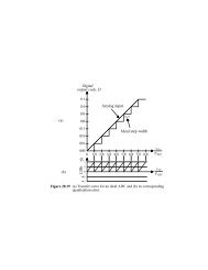The overlapping portion of the entry and descent phase altitude and descent speed profiles are shown in Fig. 19. It ARTICLE IN PRESS B. Kazeminejad et al. / Planetary and Space Science 55 (2007) 1845–1876 Altitude [km] above Impact Point Altitude Residual: Entry - Descent [m] 180 170 160 150 140 130 120 110 100 90 80 5 10 15 20 25 30 Time [min] past Interface Epoch: UTC: 2005-01-14T09:05:52.523 200 100 0 -100 -200 -300 -400 -500 can be seen that the modifications of the initial state vector ensures a smooth transition between the two phases. The difference between the two reconstructed altitude profiles are less than 0.6 km (in the overlapping region of ca. 147–100 km), which is shown in the residual plot in the lower panel of the same figure. 7. Vehicle roll rate T0 Drogue 7.1. Vehicle roll during entry ENTRY DESCENT -600 6 8 10 12 14 Time [min] 16 18 20 22 past Interface Epoch: UTC: 2005-01-14T09:05:52.523 Fig. 19. Comparison of reconstructed altitude profiles from the entry phase reconstruction (dashed thick line) and the descent phase reconstruction (solid line). The lower panel shows the corresponding altitude residuals in the overlapping altitude region. The Huygens probe postseparation axial and lateral velocity as well as the roll rate 5 were reconstructed from the Cassini bounce back reaction and the measurements of the 5 Note that in various Huygens papers the probe roll rate is also referred to as probe ‘‘spin’’.
Aerodynamic Deceleration [m/s 2 ] 6 5.5 5 4.5 4 3.5 3 2.5 2 1.5 x 10 -4 magnetometer instrument subsystem aboard Cassini (Project Team, 2005). The roll rate reconstruction yielded a counter-clockwise (viewed from the back of the probe into the velocity direction) rotation of 7.5 rpm. This initial rotation is a typical means to achieve a certain attitude control for planetary entry probes and to ensure stability during the coast phase and furthermore null out any lift and side forces during the atmospheric entry (Lorenz, 2006). The misalignment between the vehicle’s body axis (defined by the aeroshell symmetry axis) and the principal axis (defined by the aeroshell mass distribution) can be seen in the non-zero products of inertia, which are listed in the lower panel of Fig. 2. The resulting deviation moments as well as external torques caused a probe nutation motion, which can be clearly seen in the HASI servo accelerometer measurements taken prior to the start of the deceleration pulse as shown in Fig. 20. From the periodic oscillations a coning frequency of f coning ¼ 0:0889 Hz can be derived. Keeping in mind that due to the axis definition the maximum moment of inertia is along the probe X-axis the vehicle roll rate can be derived using the relation (Spencer et al., 2005) oconing ¼ 1 -4.5 -4 -3.5 -3 -2.5 -2 -1.5 -1 -0.5 0 0.5 I xx 1 2 ðI zz þ I yyÞ oroll. (25) Substituting the moment of inertia ratio and the measured coning frequency f coning ¼ 0:0889 Hz yields a vehicle roll rate of oroll ¼ 7:28 rpm. Note that this value is very close to the results of the preflight simulation, which predicted a value in the range of 7.281–7.298 rpm (Ortiz, 2004). A comparison with the reconstructed value of 7.5 rpm, however, suggests that a roll damping of about 0.22 rpm ARTICLE IN PRESS XSERVO CASU Time [min] past Interface Epoch UTC: 2005-01-14T09:05:52.523 Fig. 20. HASI servo accelerometer measurements prior to the deceleration pulse. Due to the high sensitivity of the accelerometer the probe coning motion can be seen. One can clearly see a constant coning frequency of 0.0889 Hz, which allows to calculate the vehicle roll rate during that time. B. Kazeminejad et al. / Planetary and Space Science 55 (2007) 1845–1876 1865 took place. The very low atmospheric density above 1250 km suggests that atmospheric roll damping effects (i.e., viscous roll damping due to energy dissipation within the boundary layer) could not have been strong enough to explain the observed change. One possible effect, which could partially cause a change in roll rate are solar pressure torques. A quantitative estimation of this torque throughout the entire coast phase would, however, require a detailed analysis, which is beyond the scope of this work and will be subject to future analysis. 7.2. Vehicle roll during descent The vehicle roll rate during the probe descent phase is reconstructed based on two data sets: (1) the RASU measurements and (2) the telemetry data of the Automatic Gain Control (AGC) unit, part of the Huygens receiver onboard Cassini. Note that this paper is restricted to a brief overview of descent phase roll rate reconstruction effort. For a more extensive and detailed description on this topic the reader is referred to Pérez-Ayu´car et al. (2005c). The RASU is a suite of two highly sensitive accelerometers sharing a common design with the CASU but mounted offset from the probe symmetry axis and tuned to measure a much smaller range of accelerations (0–120 mg). The RASU was sampled at 4 Hz and had an accuracy of 0.47 mg. Raw measurements were used by the onboard processor to compute a near real time roll rate estimation that was distributed to the instruments in the Data Descent Broadcast (DDB). 6 A DDB independent roll rate reconstruction based on the reduction of the raw RASU measurements as shown in Fig. 21 is presented here. The raw data are treated with a median smoothing algorithm, which filters out the measurement noise created by the recording of attitude disturbance accelerations. Assuming that the disturbed radial acceleration component is equally distributed around the ideal centrifugal component, a smoothed windowed median filter provides a good estimation of the actual instantaneous radial acceleration. It is important to note that the RASU was designed to provide only positive acceleration measurements. From the smoothed radial accelerations the vehicle roll rate is then derived according to rffiffiffiffiffiffi oroll ðrpmÞ ¼ 2p D , (26) 60 acf where D is the radial distance of the RASU with respect to the vehicle center of mass and acf is the centrifugal acceleration. For RASU-B, D ¼ 412 mm under the main chute (i.e., front shield and DISR cover jettisoned) and D ¼ 411 mm under the stabilizer chute. 6 A subset of housekeeping data were broadcasted every 2 s to all the instruments for their real time use during descent. This data set is referred to as DDB and comprised the mission time, altitude and the real-time derived roll rate. It was used by the instruments to optimize their measurement cycles.
Page 1 and 2: Planetary and Space Science 55 (200
Page 3 and 4: was separated from Cassini on the t
Page 5 and 6: EXPERIMENT PLATFORM FRONT SHIELD AF
Page 7 and 8: drive the mass from its displaced p
Page 9 and 10: initially thought to be entirely lo
Page 11 and 12: Altitude [km] above Ref. Surface of
Page 13 and 14: Altitude [km] Altitude [km] 1200 10
Page 15 and 16: 4.2. Discussion of reconstruction r
Page 17 and 18: West Longitude [deg] Latitude [deg]
Page 19: 2 km. The scales of the surface fea
Page 23 and 24: therefore be considered as approxim
Page 25 and 26: Table 4 (continued ) ARTICLE IN PRE
Page 31 and 32: leading truncation error term. Tech

Huygens' entry and descent through Titan's atmosphere ...

Create successful ePaper yourself

Delete template?

Save as template?