Chapter 2 / Atomic Structure and Interatomic Bonding

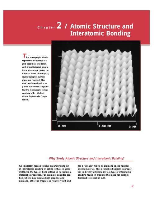
This micrograph, which
represents the surface of a
gold specimen, was taken
with a sophisticated atomic
force microscope (AFM). Individual
atoms for this (111)
crystallographic surface
plane are resolved. Also
note the dimensional scale
(in the nanometer range) below
the micrograph. (Image
courtesy of Dr. Michael
Green, TopoMetrix Corporation.)
Chapter2 / Atomic Structure and
Interatomic Bonding
An important reason to have an understanding
of interatomic bonding in solids is that, in some
instances, the type of bond allows us to explain a
material’s properties. For example, consider carbon,
which may exist as both graphite and
diamond. Whereas graphite is relatively soft and
Why Study Atomic Structure and Interatomic Bonding?
has a ‘‘greasy’’ feel to it, diamond is the hardest
known material. This dramatic disparity in properties
is directly attributable to a type of interatomic
bonding found in graphite that does not exist in
diamond (see Section 3.9).
9

Learning Objectives
After careful study of this chapter you should be able to do the following:
1. Name the two atomic models cited, and note the
differences between them.
2. Describe the important quantum-mechanical
principle that relates to electron energies.
3. (a) Schematically plot attractive, repulsive, and
net energies versus interatomic separation
for two atoms or ions.
2.1 INTRODUCTION
ATOMIC STRUCTURE
2.2 FUNDAMENTAL CONCEPTS
10
(b) Note on this plot the equilibrium separation
and the bonding energy.
4. (a) Briefly describe ionic, covalent, metallic, hydrogen,
and van der Waals bonds.
(b) Note what materials exhibit each of these
bonding types.
Some of the important properties of solid materials depend on geometrical atomic
arrangements, and also the interactions that exist among constituent atoms or
molecules. This chapter, by way of preparation for subsequent discussions, considers
several fundamental and important concepts, namely: atomic structure, electron
configurations in atoms and the periodic table, and the various types of primary
and secondary interatomic bonds that hold together the atoms comprising a solid.
These topics are reviewed briefly, under the assumption that some of the material
is familiar to the reader.
Each atom consists of a very small nucleus composed of protons and neutrons,
which is encircled by moving electrons. Both electrons and protons are electrically
charged, the charge magnitude being 1.60 10 19 C, which is negative in sign for
electrons and positive for protons; neutrons are electrically neutral. Masses for
these subatomic particles are infinitesimally small; protons and neutrons have approximately
the same mass, 1.67 10 27 kg, which is significantly larger than that
of an electron, 9.11 10 31 kg.
Each chemical element is characterized by the number of protons in the nucleus,
or the atomic number (Z). 1 For an electrically neutral or complete atom, the atomic
number also equals the number of electrons. This atomic number ranges in integral
units from 1 for hydrogen to 92 for uranium, the highest of the naturally occurring
elements.
The atomic mass (A) of a specific atom may be expressed as the sum of the
masses of protons and neutrons within the nucleus. Although the number of protons
is the same for all atoms of a given element, the number of neutrons (N) may be
variable. Thus atoms of some elements have two or more different atomic masses,
which are called isotopes. The atomic weight of an element corresponds to the
weighted average of the atomic masses of the atom’s naturally occurring isotopes. 2
The atomic mass unit (amu) may be used for computations of atomic weight. A
scale has been established whereby 1 amu is defined as of the atomic mass of
1 Terms appearing in boldface type are defined in the Glossary, which follows Appendix E.
2 The term ‘‘atomic mass’’ is really more accurate than ‘‘atomic weight’’ inasmuch as, in this
context, we are dealing with masses and not weights. However, atomic weight is, by convention,
the preferred terminology, and will be used throughout this book. The reader should
note that it is not necessary to divide molecular weight by the gravitational constant.

2.3 Electrons in Atoms ● 11
the most common isotope of carbon, carbon 12 ( 12C) (A 12.00000). Within this
scheme, the masses of protons and neutrons are slightly greater than unity, and
A Z N (2.1)
The atomic weight of an element or the molecular weight of a compound may be
specified on the basis of amu per atom (molecule) or mass per mole of material.
In one mole of a substance there are 6.023 1023 (Avogadro’s number) atoms or
molecules. These two atomic weight schemes are related through the following
equation:
1 amu/atom (or molecule) 1 g/mol
For example, the atomic weight of iron is 55.85 amu/atom, or 55.85 g/mol. Sometimes
use of amu per atom or molecule is convenient; on other occasions g (or kg)/mol
is preferred; the latter is used in this book.
2.3 ELECTRONS IN ATOMS
ATOMIC MODELS
During the latter part of the nineteenth century it was realized that many phenomena
involving electrons in solids could not be explained in terms of classical mechanics.
What followed was the establishment of a set of principles and laws that govern
systems of atomic and subatomic entities that came to be known as quantum
mechanics. An understanding of the behavior of electrons in atoms and crystalline
solids necessarily involves the discussion of quantum-mechanical concepts. However,
a detailed exploration of these principles is beyond the scope of this book,
and only a very superficial and simplified treatment is given.
One early outgrowth of quantum mechanics was the simplified Bohr atomic
model, in which electrons are assumed to revolve around the atomic nucleus in
discrete orbitals, and the position of any particular electron is more or less well
defined in terms of its orbital. This model of the atom is represented in Figure 2.1.
Another important quantum-mechanical principle stipulates that the energies
of electrons are quantized; that is, electrons are permitted to have only specific
values of energy. An electron may change energy, but in doing so it must make a
quantum jump either to an allowed higher energy (with absorption of energy) or
to a lower energy (with emission of energy). Often, it is convenient to think of
these allowed electron energies as being associated with energy levels or states.
Orbital electron
Nucleus
FIGURE 2.1 Schematic representation of
the Bohr atom.

12 ● Chapter 2 / Atomic Structure and Interatomic Bonding
FIGURE 2.2 (a) The
first three electron
energy states for the
Bohr hydrogen atom.
(b) Electron energy
states for the first three
shells of the wavemechanical
hydrogen
atom. (Adapted from
W. G. Moffatt, G. W.
Pearsall, and J. Wulff,
The Structure and
Properties of Materials,
Vol. I, Structure, p. 10.
Copyright © 1964 by
John Wiley & Sons,
New York. Reprinted
by permission of John
Wiley & Sons, Inc.)
Energy (eV)
1.5
3.4
5
10
13.6
15
0 0
n = 3
n = 2
3d
3p
3s
2p
2s
n = 1 1s
(a) (b)
1 10 18
2 10 18
These states do not vary continuously with energy; that is, adjacent states are
separated by finite energies. For example, allowed states for the Bohr hydrogen
atom are represented in Figure 2.2a. These energies are taken to be negative,
whereas the zero reference is the unbound or free electron. Of course, the single
electron associated with the hydrogen atom will fill only one of these states.
Thus, the Bohr model represents an early attempt to describe electrons in atoms,
in terms of both position (electron orbitals) and energy (quantized energy levels).
This Bohr model was eventually found to have some significant limitations
because of its inability to explain several phenomena involving electrons. A resolution
was reached with a wave-mechanical model, in which the electron is considered
to exhibit both wavelike and particle-like characteristics. With this model, an electron
is no longer treated as a particle moving in a discrete orbital; but rather,
position is considered to be the probability of an electron’s being at various locations
around the nucleus. In other words, position is described by a probability distribution
or electron cloud. Figure 2.3 compares Bohr and wave-mechanical models for the
hydrogen atom. Both these models are used throughout the course of this book;
the choice depends on which model allows the more simple explanation.
QUANTUM NUMBERS
Using wave mechanics, every electron in an atom is characterized by four parameters
called quantum numbers. The size, shape, and spatial orientation of an electron’s
probability density are specified by three of these quantum numbers. Furthermore,
Bohr energy levels separate into electron subshells, and quantum numbers dictate
the number of states within each subshell. Shells are specified by a principal quantum
number n, which may take on integral values beginning with unity; sometimes these
shells are designated by the letters K, L, M, N, O, and so on, which correspond,
respectively, to n 1,2,3,4,5,...,asindicated in Table 2.1. It should also be
Energy (J)

Probability
1.0
Orbital electron Nucleus
0
Distance from nucleus
(a) (b)
2.3 Electrons in Atoms ● 13
FIGURE 2.3 Comparison of
the (a) Bohr and (b) wavemechanical
atom models in
terms of electron
distribution. (Adapted from
Z. D. Jastrzebski, The
Nature and Properties of
Engineering Materials, 3rd
edition, p. 4. Copyright ©
1987 by John Wiley & Sons,
New York. Reprinted by
permission of John Wiley &
Sons, Inc.)
Table 2.1 The Number of Available Electron States in Some of the
Electron Shells and Subshells
Principal
Quantum Shell
Number Number of Electrons
Number n Designation Subshells of States Per Subshell Per Shell
1 K s 1 2 2
2 L
s 1 2
p 3 6
s 1 2
3 M p 3 6 18
d 5 10
4 N
s 1 2
p 3 6
d 5 10
f 7 14
8
32

14 ● Chapter 2 / Atomic Structure and Interatomic Bonding
noted that this quantum number, and it only, is also associated with the Bohr model.
This quantum number is related to the distance of an electron from the nucleus,
or its position.
The second quantum number, l, signifies the subshell, which is denoted by a
lowercase letter—an s, p, d, orf; it is related to the shape of the electron subshell.
In addition, the number of these subshells is restricted by the magnitude of n.
Allowable subshells for the several n values are also presented in Table 2.1. The
number of energy states for each subshell is determined by the third quantum
number, m l. For an s subshell, there is a single energy state, whereas for p, d, and
f subshells, three, five, and seven states exist, respectively (Table 2.1). In the absence
of an external magnetic field, the states within each subshell are identical. However,
when a magnetic field is applied these subshell states split, each state assuming a
slightly different energy.
Associated with each electron is a spin moment, which must be oriented either
up or down. Related to this spin moment is the fourth quantum number, m s, for
which two values are possible (and ), one for each of the spin orientations.
Thus, the Bohr model was further refined by wave mechanics, in which the
introduction of three new quantum numbers gives rise to electron subshells within
each shell. A comparison of these two models on this basis is illustrated, for the
hydrogen atom, in Figures 2.2a and 2.2b.
A complete energy level diagram for the various shells and subshells using the
wave-mechanical model is shown in Figure 2.4. Several features of the diagram are
worth noting. First, the smaller the principal quantum number, the lower the energy
level; for example, the energy of a 1s state is less than that of a 2s state, which in
turn is lower than the 3s. Second, within each shell, the energy of a subshell level
increases with the value of the l quantum number. For example, the energy of a
3d state is greater than a 3p, which is larger than 3s. Finally, there may be overlap
in energy of a state in one shell with states in an adjacent shell, which is especially
true of d and f states; for example, the energy of a 3d state is greater than that for
a4s.
Energy
s
1
p
s
d
p
s
p
s
p
s
Principal quantum number, n
f
d
f
d
f
d
p
s
d
p
s
2 3 4 5 6 7
FIGURE 2.4 Schematic
representation of the relative
energies of the electrons for the
various shells and subshells. (From
K. M. Ralls, T. H. Courtney, and J.
Wulff, Introduction to Materials
Science and Engineering, p. 22.
Copyright © 1976 by John Wiley &
Sons, New York. Reprinted by
permission of John Wiley & Sons,
Inc.)

ELECTRON CONFIGURATIONS
2.3 Electrons in Atoms ● 15
The preceding discussion has dealt primarily with electron states—values of energy
that are permitted for electrons. To determine the manner in which these states
are filled with electrons, we use the Pauli exclusion principle, another quantummechanical
concept. This principle stipulates that each electron state can hold no
more than two electrons, which must have opposite spins. Thus, s, p, d, and f
subshells may each accommodate, respectively, a total of 2, 6, 10, and 14 electrons;
Table 2.1 summarizes the maximum number of electrons that may occupy each of
the first four shells.
Of course, not all possible states in an atom are filled with electrons. For most
atoms, the electrons fill up the lowest possible energy states in the electron shells
and subshells, two electrons (having opposite spins) per state. The energy structure
for a sodium atom is represented schematically in Figure 2.5. When all the electrons
occupy the lowest possible energies in accord with the foregoing restrictions, an
atom is said to be in its ground state. However, electron transitions to higher energy
states are possible, as discussed in Chapters 12 and 19. The electron configuration
or structure of an atom represents the manner in which these states are occupied.
In the conventional notation the number of electrons in each subshell is indicated
by a superscript after the shell–subshell designation. For example, the electron
configurations for hydrogen, helium, and sodium are, respectively, 1s 1 ,1s 2 , and
1s 2 2s 2 2p 6 3s 1 . Electron configurations for some of the more common elements are
listed in Table 2.2.
At this point, comments regarding these electron configurations are necessary.
First, the valence electrons are those that occupy the outermost filled shell. These
electrons are extremely important; as will be seen, they participate in the bonding
between atoms to form atomic and molecular aggregates. Furthermore, many of
the physical and chemical properties of solids are based on these valence electrons.
In addition, some atoms have what are termed ‘‘stable electron configurations’’;
that is, the states within the outermost or valence electron shell are completely
filled. Normally this corresponds to the occupation of just the s and p states for
the outermost shell by a total of eight electrons, as in neon, argon, and krypton;
one exception is helium, which contains only two 1s electrons. These elements (Ne,
Ar, Kr, and He) are the inert, or noble, gases, which are virtually unreactive
chemically. Some atoms of the elements that have unfilled valence shells assume
Increasing energy
3s
2s
1s
3p
2p
FIGURE 2.5 Schematic representation of the
filled energy states for a sodium atom.

16 ● Chapter 2 / Atomic Structure and Interatomic Bonding
Table 2.2 A Listing of the Expected Electron Configurations
for Some of the Common Elementsa Atomic
Element Symbol Number Electron Configuration
Hydrogen H 1 1s1 Helium He 2 1s2 Lithium Li 3 1s22s 1
Beryllium Be 4 1s22s 2
Boron B 5 1s22s 22p1 Carbon C 6 1s22s 22p2 Nitrogen N 7 1s22s 22p3 Oxygen O 8 1s22s 22p4 Fluorine F 9 1s22s 22p5 Neon Ne 10 1s22s 22p6 Sodium Na 11 1s22s 22p63s 1
Magnesium Mg 12 1s22s 22p63s 2
Aluminum Al 13 1s22s 22p63s 23p1 Silicon Si 14 1s22s 22p63s 23p2 Phosphorus P 15 1s22s 22p63s 23p3 Sulfur S 16 1s22s 22p63s 23p4 Chlorine Cl 17 1s22s 22p63s 23p5 Argon Ar 18 1s22s 22p63s 23p6 Potassium K 19 1s22s 22p63s 23p64s 1
Calcium Ca 20 1s22s 22p63s 23p64s 2
Scandium Sc 21 1s22s 22p63s 23p63d 14s2 Titanium Ti 22 1s22s 22p63s 23p63d 24s2 Vanadium V 23 1s22s 22p63s 23p63d 34s2 Chromium Cr 24 1s22s 22p63s 23p63d 54s1 Manganese Mn 25 1s22s 22p63s 23p63d 54s2 Iron Fe 26 1s22s 22p63s 23p63d 64s2 Cobalt Co 27 1s22s 22p63s 23p63d 74s2 Nickel Ni 28 1s22s 22p63s 23p63d 84s2 Copper Cu 29 1s22s 22p63s 23p63d 104s1 Zinc Zn 30 1s22s 22p63s 23p63d 104s2 Gallium Ga 31 1s22s 22p63s 23p63d 104s24p1 Germanium Ge 32 1s22s 22p63s 23p63d 104s24p2 Arsenic As 33 1s22s 22p63s 23p63d 104s24p3 Selenium Se 34 1s22s 22p63s 23p63d 104s24p4 Bromine Br 35 1s22s 22p63s 23p63d 104s24p5 Krypton Kr 36 1s22s 22p63s 23p63d 104s24p6 a When some elements covalently bond, they form sp hybrid bonds. This is especially
true for C, Si, and Ge.
stable electron configurations by gaining or losing electrons to form charged ions,
or by sharing electrons with other atoms. This is the basis for some chemical
reactions, and also for atomic bonding in solids, as explained in Section 2.6.
Under special circumstances, the s and p orbitals combine to form hybrid sp n
orbitals, where n indicates the number of p orbitals involved, which may have a
value of 1, 2, or 3. The 3A, 4A, and 5A group elements of the periodic table (Figure
2.6) are those which most often form these hybrids. The driving force for the
formation of hybrid orbitals is a lower energy state for the valence electrons. For
carbon the sp 3 hybrid is of primary importance in organic and polymer chemistries.

2.4 THE PERIODIC TABLE
IA
1
H
1.0080
3
Li
6.939
11
Na
22.990
19
K
39.102
37
Rb
85.47
55
Cs
132.91
87
Fr
(223)
IIA
4
Be
9.0122
12
Mg
24.312
20
Ca
40.08
38
Sr
87.62
56
Ba
137.34
88
Ra
(226)
21
Sc
44.956
39
Y
88.91
22
Ti
47.90
40
Zr
91.22
72
Hf
178.49
57
La
138.91
89
Ac
(227)
Key
29
Cu
63.54
23
V
50.942
41
Nb
92.91
73
Ta
180.95
58
Ce
140.12
90
Th
232.04
Atomic number
Symbol
Atomic weight
IIIB IVB VB VIB VIIB
Rare
earth
series
Actinide
series
Rare earth series
Actinide series
24
Cr
51.996
42
Mo
95.94
74
W
183.85
59
Pr
140.91
91
Pa
(231)
25
Mn
54.938
43
Tc
(99)
75
Re
186.2
60
Nd
144.24
92
U
238.03
26
Fe
55.847
44
Ru
101.07
76
Os
190.2
61
Pm
(145)
93
Np
(237)
VIII
27
Co
58.933
45
Rh
102.91
77
Ir
192.2
62
Sm
150.35
94
Pu
(242)
Metal
Nonmetal
Intermediate
28
Ni
58.71
46
Pd
106.4
78
Pt
195.09
63
Eu
151.96
95
Am
(243)
IB IIB
29
Cu
63.54
47
Ag
107.87
79
Au
196.97
64
Gd
157.25
96
Cm
(247)
30
Zn
65.37
48
Cd
112.40
80
Hg
200.59
65
Tb
158.92
97
Bk
(247)
5
B
10.811
13
Al
26.982
31
Ga
69.72
49
In
114.82
81
Tl
204.37
66
Dy
162.50
98
Cf
(249)
2.4 The Periodic Table ● 17
The shape of the sp 3 hybrid is what determines the 109 (or tetrahedral) angle
found in polymer chains (Chapter 4).
All the elements have been classified according to electron configuration in the
periodic table (Figure 2.6). Here, the elements are situated, with increasing atomic
number, in seven horizontal rows called periods. The arrangement is such that all
elements that are arrayed in a given column or group have similar valence electron
structures, as well as chemical and physical properties. These properties change
gradually and systematically, moving horizontally across each period.
The elements positioned in Group 0, the rightmost group, are the inert gases,
which have filled electron shells and stable electron configurations. Group VIIA
and VIA elements are one and two electrons deficient, respectively, from having
stable structures. The Group VIIA elements (F, Cl, Br, I, and At) are sometimes
termed the halogens. The alkali and the alkaline earth metals (Li, Na, K, Be, Mg,
Ca, etc.) are labeled as Groups IA and IIA, having, respectively, one and two
electrons in excess of stable structures. The elements in the three long periods,
Groups IIIB through IIB, are termed the transition metals, which have partially
filled d electron states and in some cases one or two electrons in the next higher
energy shell. Groups IIIA, IVA, and VA (B, Si, Ge, As, etc.) display characteristics
that are intermediate between the metals and nonmetals by virtue of their valence
electron structures.
IIIA IVA VA VIA VIIA
6
C
12.011
14
Si
28.086
32
Ge
72.59
50
Sn
118.69
82
Pb
207.19
67
Ho
164.93
99
Es
(254)
7
N
14.007
15
P
30.974
33
As
74.922
51
Sb
121.75
83
Bi
208.98
68
Er
167.26
100
Fm
(253)
8
O
15.999
16
S
32.064
34
Se
78.96
52
Te
127.60
84
Po
(210)
69
Tm
168.93
101
Md
(256)
FIGURE 2.6 The periodic table of the elements. The numbers in parentheses are
the atomic weights of the most stable or common isotopes.
9
F
18.998
17
Cl
35.453
35
Br
79.91
53
I
126.90
85
At
(210)
70
Yb
173.04
102
No
(254)
0
2
He
4.0026
10
Ne
20.183
18
Ar
39.948
36
Kr
83.80
54
Xe
131.30
86
Rn
(222)
71
Lu
174.97
103
Lw
(257)

18 ● Chapter 2 / Atomic Structure and Interatomic Bonding
IA
1
H
2.1
3 4
Li Be
1.0 1.5
11 12
Na Mg
0.9 1.2
19 20
K Ca
0.8 1.0
37
Rb
0.8
IIA
38
Sr
1.0
21
Sc
1.3
39
Y
1.2
55 56 57 71
Cs Ba La Lu
0.7 0.9 1.1 1.2
87 88 89 102
Fr Ra Ac No
0.7 0.9 1.1 1.7
IIIB IVB VB VIB VIIB
22
Ti
1.5
40
Zr
1.4
72
Hf
1.3
23
V
1.6
41
Nb
1.6
73
Ta
1.5
24
Cr
1.6
42
Mo
1.8
74
W
1.7
25
Mn
1.5
43
Tc
1.9
75
Re
1.9
26
Fe
1.8
44
Ru
2.2
76
Os
2.2
27
Co
1.8
45
Rh
2.2
77
Ir
2.2
As may be noted from the periodic table, most of the elements really come
under the metal classification. These are sometimes termed electropositive elements,
indicating that they are capable of giving up their few valence electrons to become
positively charged ions. Furthermore, the elements situated on the right-hand side
of the table are electronegative; that is, they readily accept electrons to form
negatively charged ions, or sometimes they share electrons with other atoms. Figure
2.7 displays electronegativity values that have been assigned to the various elements
arranged in the periodic table. As a general rule, electronegativity increases in
moving from left to right and from bottom to top. Atoms are more likely to accept
electrons if their outer shells are almost full, and if they are less ‘‘shielded’’ from
(i.e., closer to) the nucleus.
ATOMIC BONDING IN SOLIDS
2.5 BONDING FORCES AND ENERGIES
VIII
28
Ni
1.8
46
Pd
2.2
78
Pt
2.2
IB IIB
29
Cu
1.9
47
Ag
1.9
79
Au
2.4
An understanding of many of the physical properties of materials is predicated on
a knowledge of the interatomic forces that bind the atoms together. Perhaps the
principles of atomic bonding are best illustrated by considering the interaction
between two isolated atoms as they are brought into close proximity from an infinite
separation. At large distances, the interactions are negligible; but as the atoms
approach, each exerts forces on the other. These forces are of two types, attractive
and repulsive, and the magnitude of each is a function of the separation or interatomic
distance. The origin of an attractive force FA depends on the particular
type of bonding that exists between the two atoms. Its magnitude varies with the
distance, as represented schematically in Figure 2.8a. Ultimately, the outer electron
shells of the two atoms begin to overlap, and a strong repulsive force FR comes
into play. The net force FN between the two atoms is just the sum of both attractive
and repulsive components; that is,
FN FA FR (2.2)
30
Zn
1.6
48
Cd
1.7
80
Hg
1.9
IIIA IVA VA VIA VIIA
FIGURE 2.7 The electronegativity values for the elements. (Adapted from Linus
Pauling, The Nature of the Chemical Bond, 3rd edition. Copyright 1939 and 1940,
3rd edition copyright © 1960, by Cornell University. Used by permission of the
publisher, Cornell University Press.)
5
B
2.0
13
Al
1.5
31
Ga
1.6
49
In
1.7
81
Tl
1.8
6
C
2.5
14
Si
1.8
32
Ge
1.8
50
Sn
1.8
82
Pb
1.8
7
N
3.0
15
P
2.1
33
As
2.0
51
Sb
1.9
83
Bi
1.9
8
O
3.5
16
S
2.5
34
Se
2.4
52
Te
2.1
84
Po
2.0
9
F
4.0
17
Cl
3.0
35
Br
2.8
53
I
2.5
85
At
2.2
0
2
He
10
Ne
18
Ar
36
Kr
54
Xe
86
Rn

Force F
Attraction
Repulsion
Attraction Repulsion
Potential energy E
+
0
+
0
E 0
r 0
2.5 Bonding Forces and Energies ● 19
which is also a function of the interatomic separation, as also plotted in Figure
2.8a. When FA and FR balance, or become equal, there is no net force; that is,
FA FR 0 (2.3)
Then a state of equilibrium exists. The centers of the two atoms will remain separated
by the equilibrium spacing r0, as indicated in Figure 2.8a. For many atoms, r0 is
approximately 0.3 nm (3 A˚ ). Once in this position, the two atoms will counteract
any attempt to separate them by an attractive force, or to push them together by
a repulsive action.
Sometimes it is more convenient to work with the potential energies between
two atoms instead of forces. Mathematically, energy (E) and force (F) are related as
Or, for atomic systems,
Attractive force F A
Repulsive force F R
Net force F N
(a)
Repulsive energy E R
Net energy E N
Attractive energy E A
(b)
Interatomic separation r
Interatomic separation r
EN r
r
E Fdr (2.4)
F N dr (2.5)
FA dr r
FR dr (2.6)
EA ER (2.7)
in which EN, EA, and ER are respectively the net, attractive, and repulsive energies
for two isolated and adjacent atoms.
FIGURE 2.8 (a) The
dependence of repulsive,
attractive, and net forces on
interatomic separation for
two isolated atoms. (b) The
dependence of repulsive,
attractive, and net potential
energies on interatomic
separation for two isolated
atoms.

20 ● Chapter 2 / Atomic Structure and Interatomic Bonding
Figure 2.8b plots attractive, repulsive, and net potential energies as a function
of interatomic separation for two atoms. The net curve, which is again the sum of
the other two, has a potential energy trough or well around its minimum. Here,
the same equilibrium spacing, r 0, corresponds to the separation distance at the
minimum of the potential energy curve. The bonding energy for these two atoms,
E 0, corresponds to the energy at this minimum point (also shown in Figure 2.8b);
it represents the energy that would be required to separate these two atoms to an
infinite separation.
Although the preceding treatment has dealt with an ideal situation involving
only two atoms, a similar yet more complex condition exists for solid materials
because force and energy interactions among many atoms must be considered.
Nevertheless, a bonding energy, analogous to E 0 above, may be associated with
each atom. The magnitude of this bonding energy and the shape of the energyversus-interatomic
separation curve vary from material to material, and they both
depend on the type of atomic bonding. Furthermore, a number of material properties
depend on E 0, the curve shape, and bonding type. For example, materials having
large bonding energies typically also have high melting temperatures; at room
temperature, solid substances are formed for large bonding energies, whereas for
small energies the gaseous state is favored; liquids prevail when the energies are
of intermediate magnitude. In addition, as discussed in Section 7.3, the mechanical
stiffness (or modulus of elasticity) of a material is dependent on the shape of its
force-versus-interatomic separation curve (Figure 7.7). The slope for a relatively
stiff material at the r r 0 position on the curve will be quite steep; slopes are
shallower for more flexible materials. Furthermore, how much a material expands
upon heating or contracts upon cooling (that is, its linear coefficient of thermal
expansion) is related to the shape of its E 0-versus-r 0 curve (see Section 17.3). A
deep and narrow ‘‘trough,’’ which typically occurs for materials having large bonding
energies, normally correlates with a low coefficient of thermal expansion and relatively
small dimensional alterations for changes in temperature.
Three different types of primary or chemical bond are found in solids—ionic,
covalent, and metallic. For each type, the bonding necessarily involves the valence
electrons; furthermore, the nature of the bond depends on the electron structures
of the constituent atoms. In general, each of these three types of bonding arises
from the tendency of the atoms to assume stable electron structures, like those of
the inert gases, by completely filling the outermost electron shell.
Secondary or physical forces and energies are also found in many solid materials;
they are weaker than the primary ones, but nonetheless influence the physical
properties of some materials. The sections that follow explain the several kinds of
primary and secondary interatomic bonds.
2.6 PRIMARY INTERATOMIC BONDS
IONIC BONDING
Perhaps ionic bonding is the easiest to describe and visualize. It is always found in
compounds that are composed of both metallic and nonmetallic elements, elements
that are situated at the horizontal extremities of the periodic table. Atoms of a
metallic element easily give up their valence electrons to the nonmetallic atoms.
In the process all the atoms acquire stable or inert gas configurations and, in
addition, an electrical charge; that is, they become ions. Sodium chloride (NaCl)
is the classical ionic material. A sodium atom can assume the electron structure of
neon (and a net single positive charge) by a transfer of its one valence 3s electron

Na +
Cl
Na +
Cl
Cl
Na +
Cl
Na +
Coulombic bonding force
Na +
Cl
Na +
Cl
Cl
Na +
Cl
Na +
Na +
Cl
Na +
Cl
2.6 Primary Interatomic Bonds ● 21
to a chlorine atom. After such a transfer, the chlorine ion has a net negative charge
and an electron configuration identical to that of argon. In sodium chloride, all the
sodium and chlorine exist as ions. This type of bonding is illustrated schematically
in Figure 2.9.
The attractive bonding forces are coulombic; that is, positive and negative ions,
by virtue of their net electrical charge, attract one another. For two isolated ions,
the attractive energy E A is a function of the interatomic distance according to 3
E A A
r
An analogous equation for the repulsive energy is
FIGURE 2.9 Schematic representation of ionic
bonding in sodium chloride (NaCl).
E R B
r n
(2.8)
(2.9)
In these expressions, A, B, and n are constants whose values depend on the particular
ionic system. The value of n is approximately 8.
Ionic bonding is termed nondirectional, that is, the magnitude of the bond is
equal in all directions around an ion. It follows that for ionic materials to be stable,
all positive ions must have as nearest neighbors negatively charged ions in a threedimensional
scheme, and vice versa. The predominant bonding in ceramic materials
is ionic. Some of the ion arrangements for these materials are discussed in Chapter 3.
Bonding energies, which generally range between 600 and 1500 kJ/mol (3 and
8 eV/atom), are relatively large, as reflected in high melting temperatures. 4 Table
3 The constant A in Equation 2.8 is equal to
1
(Z1e)(Z2e)
40
where 0 is the permittivity of a vacuum (8.85 10 12 F/m), Z1 and Z2 are the valences of
the two ion types, and e is the electronic charge (1.602 10 19 C).
4 Sometimes bonding energies are expressed per atom or per ion. Under these circumstances
the electron volt (eV) is a conveniently small unit of energy. It is, by definition, the energy
imparted to an electron as it falls through an electric potential of one volt. The joule equivalent
of the electron volt is as follows: 1.602 10 19 J 1eV.

22 ● Chapter 2 / Atomic Structure and Interatomic Bonding
Table 2.3 Bonding Energies and Melting Temperatures for
Various Substances
Bonding Energy Melting
kJ/mol eV/Atom, Temperature
Bonding Type Substance (kcal/mol) Ion, Molecule (C)
Ionic
NaCl
MgO
640 (153)
1000 (239)
3.3
5.2
801
2800
Covalent
Si
C (diamond)
450 (108)
713 (170)
4.7
7.4
1410
3550
Hg 68 (16) 0.7 39
Metallic
Al
Fe
324 (77)
406 (97)
3.4
4.2
660
1538
W 849 (203) 8.8 3410
van der Waals
Hydrogen
Ar 7.7 (1.8) 0.08 189
Cl2 31 (7.4) 0.32 101
NH3 35 (8.4) 0.36 78
H2O 51 (12.2) 0.52 0
2.3 contains bonding energies and melting temperatures for several ionic materials.
Ionic materials are characteristically hard and brittle and, furthermore, electrically
and thermally insulative. As discussed in subsequent chapters, these properties are
a direct consequence of electron configurations and/or the nature of the ionic bond.
COVALENT BONDING
In covalent bonding stable electron configurations are assumed by the sharing of
electrons between adjacent atoms. Two atoms that are covalently bonded will each
contribute at least one electron to the bond, and the shared electrons may be
considered to belong to both atoms. Covalent bonding is schematically illustrated
in Figure 2.10 for a molecule of methane (CH4). The carbon atom has four valence
electrons, whereas each of the four hydrogen atoms has a single valence electron.
Each hydrogen atom can acquire a helium electron configuration (two 1s valence
electrons) when the carbon atom shares with it one electron. The carbon now has
four additional shared electrons, one from each hydrogen, for a total of eight valence
Shared electron
from hydrogen
H
H
C
H
Shared electron
from carbon
H
FIGURE 2.10 Schematic representation of
covalent bonding in a molecule of methane
(CH4).

2.6 Primary Interatomic Bonds ● 23
electrons, and the electron structure of neon. The covalent bond is directional; that
is, it is between specific atoms and may exist only in the direction between one
atom and another that participates in the electron sharing.
Many nonmetallic elemental molecules (H2,Cl2,F2, etc.) as well as molecules
containing dissimilar atoms, such as CH4,H2O, HNO3, and HF, are covalently
bonded. Furthermore, this type of bonding is found in elemental solids such as
diamond (carbon), silicon, and germanium and other solid compounds composed
of elements that are located on the right-hand side of the periodic table, such as
gallium arsenide (GaAs), indium antimonide (InSb), and silicon carbide (SiC).
The number of covalent bonds that is possible for a particular atom is determined
by the number of valence electrons. For N valence electrons, an atom can
covalently bond with at most 8 N other atoms. For example, N7 for chlorine,
and 8 N 1, which means that one Cl atom can bond to only one other atom,
as in Cl2. Similarly, for carbon, N 4, and each carbon atom has 8 4, or
four, electrons to share. Diamond is simply the three-dimensional interconnecting
structure wherein each carbon atom covalently bonds with four other carbon atoms.
This arrangement is represented in Figure 3.16.
Covalent bonds may be very strong, as in diamond, which is very hard and has
a very high melting temperature, 3550C (6400F), or they may be very weak, as
with bismuth, which melts at about 270C (518F). Bonding energies and melting
temperatures for a few covalently bonded materials are presented in Table 2.3.
Polymeric materials typify this bond, the basic molecular structure being a long
chain of carbon atoms that are covalently bonded together with two of their available
four bonds per atom. The remaining two bonds normally are shared with other
atoms, which also covalently bond. Polymeric molecular structures are discussed
in detail in Chapter 4.
It is possible to have interatomic bonds that are partially ionic and partially
covalent, and, in fact, very few compounds exhibit pure ionic or covalent bonding.
For a compound, the degree of either bond type depends on the relative positions
of the constituent atoms in the periodic table (Figure 2.6) or the difference in their
electronegativities (Figure 2.7). The wider the separation (both horizontally—
relative to Group IVA—and vertically) from the lower left to the upper-right-hand
corner (i.e., the greater the difference in electronegativity), the more ionic the bond.
Conversely, the closer the atoms are together (i.e., the smaller the difference in
electronegativity), the greater the degree of covalency. The percent ionic character
of a bond between elements A and B (A being the most electronegative) may be
approximated by the expression
% ionic character 1 exp[(0.25)(XA XB) 2 ] 100 (2.10)
where XA and XB are the electronegativities for the respective elements.
METALLIC BONDING
Metallic bonding, the final primary bonding type, is found in metals and their alloys.
A relatively simple model has been proposed that very nearly approximates the
bonding scheme. Metallic materials have one, two, or at most, three valence electrons.
With this model, these valence electrons are not bound to any particular
atom in the solid and are more or less free to drift throughout the entire metal.
They may be thought of as belonging to the metal as a whole, or forming a ‘‘sea
of electrons’’ or an ‘‘electron cloud.’’ The remaining nonvalence electrons and
atomic nuclei form what are called ion cores, which possess a net positive charge
equal in magnitude to the total valence electron charge per atom. Figure 2.11 is a

24 ● Chapter 2 / Atomic Structure and Interatomic Bonding
2.7 SECONDARY BONDING OR
VAN DER WAALS BONDING
+
+
+
+
+
+
+
+
+
+ + + +
Sea of valence electrons
Ion cores
+
+
+
FIGURE 2.11 Schematic illustration of
metallic bonding.
schematic illustration of metallic bonding. The free electrons shield the positively
charged ion cores from mutually repulsive electrostatic forces, which they would
otherwise exert upon one another; consequently the metallic bond is nondirectional
in character. In addition, these free electrons act as a ‘‘glue’’ to hold the ion cores
together. Bonding energies and melting temperatures for several metals are listed
in Table 2.3. Bonding may be weak or strong; energies range from 68 kJ/mol (0.7
eV/atom) for mercury to 850 kJ/mol (8.8 eV/atom) for tungsten. Their respective
melting temperatures are 39 and 3410C (38 and 6170F).
Metallic bonding is found for Group IA and IIA elements in the periodic table,
and, in fact, for all elemental metals.
Some general behaviors of the various material types (i.e., metals, ceramics,
polymers) may be explained by bonding type. For example, metals are good conductors
of both electricity and heat, as a consequence of their free electrons (see
Sections 12.5, 12.6, and 17.4). By way of contrast, ionically and covalently bonded
materials are typically electrical and thermal insulators, due to the absence of large
numbers of free electrons.
Furthermore, in Section 8.5 we note that at room temperature, most metals
and their alloys fail in a ductile manner; that is, fracture occurs after the materials
have experienced significant degrees of permanent deformation. This behavior is
explained in terms of deformation mechanism (Section 8.3), which is implicitly
related to the characteristics of the metallic bond. Conversely, at room temperature
ionically bonded materials are intrinsically brittle as a consequence of the electrically
charged nature of their component ions (see Section 8.15).
Secondary, van der Waals, or physical bonds are weak in comparison to the primary
or chemical ones; bonding energies are typically on the order of only 10 kJ/mol
(0.1 eV/atom). Secondary bonding exists between virtually all atoms or molecules,
but its presence may be obscured if any of the three primary bonding types is
present. Secondary bonding is evidenced for the inert gases, which have stable

+
Atomic or molecular dipoles
+
2.7 Secondary Bonding or Van der Waals Bonding ● 25
FIGURE 2.12 Schematic illustration of van der Waals
bonding between two dipoles.
electron structures, and, in addition, between molecules in molecular structures
that are covalently bonded.
Secondary bonding forces arise from atomic or molecular dipoles. In essence,
an electric dipole exists whenever there is some separation of positive and negative
portions of an atom or molecule. The bonding results from the coulombic attraction
between the positive end of one dipole and the negative region of an adjacent one,
as indicated in Figure 2.12. Dipole interactions occur between induced dipoles,
between induced dipoles and polar molecules (which have permanent dipoles), and
between polar molecules. Hydrogen bonding, a special type of secondary bonding,
is found to exist between some molecules that have hydrogen as one of the constituents.
These bonding mechanisms are now discussed briefly.
FLUCTUATING INDUCED DIPOLE BONDS
A dipole may be created or induced in an atom or molecule that is normally
electrically symmetric; that is, the overall spatial distribution of the electrons is
symmetric with respect to the positively charged nucleus, as shown in Figure 2.13a.
All atoms are experiencing constant vibrational motion that can cause instantaneous
and short-lived distortions of this electrical symmetry for some of the atoms or
molecules, and the creation of small electric dipoles, as represented in Figure 2.13b.
One of these dipoles can in turn produce a displacement of the electron distribution
of an adjacent molecule or atom, which induces the second one also to become a
dipole that is then weakly attracted or bonded to the first; this is one type of van
der Waals bonding. These attractive forces may exist between large numbers of
atoms or molecules, which forces are temporary and fluctuate with time.
The liquefaction and, in some cases, the solidification of the inert gases and
other electrically neutral and symmetric molecules such as H2 and Cl2 are realized
because of this type of bonding. Melting and boiling temperatures are extremely
low in materials for which induced dipole bonding predominates; of all possible
intermolecular bonds, these are the weakest. Bonding energies and melting temperatures
for argon and chlorine are also tabulated in Table 2.3.
POLAR MOLECULE-INDUCED DIPOLE BONDS
Permanent dipole moments exist in some molecules by virtue of an asymmetrical
arrangement of positively and negatively charged regions; such molecules are
termed polar molecules. Figure 2.14 is a schematic representation of a hydrogen
Atomic nucleus
Electron cloud
Atomic nucleus
(a) (b)
+
Electron cloud
FIGURE 2.13 Schematic
representations of (a) an
electrically symmetric
atom and (b) an induced
atomic dipole.

26 ● Chapter 2 / Atomic Structure and Interatomic Bonding
2.8 MOLECULES
+
H
Cl
FIGURE 2.14 Schematic representation of a polar hydrogen chloride
(HCl) molecule.
chloride molecule; a permanent dipole moment arises from net positive and negative
charges that are respectively associated with the hydrogen and chlorine ends of the
HCl molecule.
Polar molecules can also induce dipoles in adjacent nonpolar molecules, and
a bond will form as a result of attractive forces between the two molecules. Furthermore,
the magnitude of this bond will be greater than for fluctuating induced dipoles.
PERMANENT DIPOLE BONDS
Van der Waals forces will also exist between adjacent polar molecules. The associated
bonding energies are significantly greater than for bonds involving induced dipoles.
The strongest secondary bonding type, the hydrogen bond, is a special case of
polar molecule bonding. It occurs between molecules in which hydrogen is covalently
bonded to fluorine (as in HF), oxygen (as in H2O), and nitrogen (as in NH3). For each HUF, HUO, or HUN bond, the single hydrogen electron is shared with
the other atom. Thus, the hydrogen end of the bond is essentially a positively
charged bare proton that is unscreened by any electrons. This highly positively
charged end of the molecule is capable of a strong attractive force with the negative
end of an adjacent molecule, as demonstrated in Figure 2.15 for HF. In essence,
this single proton forms a bridge between two negatively charged atoms. The
magnitude of the hydrogen bond is generally greater than that of the other types
of secondary bonds, and may be as high as 51 kJ/mol (0.52 eV/molecule), as shown
in Table 2.3. Melting and boiling temperatures for hydrogen fluoride and water
are abnormally high in light of their low molecular weights, as a consequence of
hydrogen bonding.
At the conclusion of this chapter, let us take a moment to discuss the concept of
a molecule in terms of solid materials. A molecule may be defined as a group of
atoms that are bonded together by strong primary bonds. Within this context, the
entirety of ionic and metallically bonded solid specimens may be considered as a
single molecule. However, this is not the case for many substances in which covalent
bonding predominates; these include elemental diatomic molecules (F 2,O 2,H 2,
etc.) as well as a host of compounds (H 2O, CO 2, HNO 3,C 6H 6,CH 4, etc.). In the
H
F
Hydrogen
bond
H
F
FIGURE 2.15 Schematic representation of hydrogen
bonding in hydrogen fluoride (HF).

Important Terms and Concepts ● 27
condensed liquid and solid states, bonds between molecules are weak secondary
ones. Consequently, molecular materials have relatively low melting and boiling
temperatures. Most of those that have small molecules composed of a few atoms
are gases at ordinary, or ambient, temperatures and pressures. On the other hand,
many of the modern polymers, being molecular materials composed of extremely
large molecules, exist as solids; some of their properties are strongly dependent on
the presence of van der Waals and hydrogen secondary bonds.
SUMMARY
This chapter began with a survey of the fundamentals of atomic structure, presenting
the Bohr and wave-mechanical models of electrons in atoms. Whereas the Bohr
model assumes electrons to be particles orbiting the nucleus in discrete paths, in
wave mechanics we consider them to be wavelike and treat electron position in
terms of a probability distribution.
Electron energy states are specified in terms of quantum numbers that give
rise to electron shells and subshells. The electron configuration of an atom corresponds
to the manner in which these shells and subshells are filled with electrons
in compliance with the Pauli exclusion principle. The periodic table of the elements
is generated by arrangement of the various elements according to valence electron
configuration.
Atomic bonding in solids may be considered in terms of attractive and repulsive
forces and energies. The three types of primary bond in solids are ionic, covalent, and
metallic. For ionic bonds, electrically charged ions are formed by the transference of
valence electrons from one atom type to another; forces are coulombic. There is a
sharing of valence electrons between adjacent atoms when bonding is covalent.
With metallic bonding, the valence electrons form a ‘‘sea of electrons’’ that is
uniformly dispersed around the metal ion cores and acts as a form of glue for them.
Both van der Waals and hydrogen bonds are termed secondary, being weak in
comparison to the primary ones. They result from attractive forces between electric
dipoles, of which there are two types—induced and permanent. For the hydrogen
bond, highly polar molecules form when hydrogen covalently bonds to a nonmetallic
element such as fluorine.
IMPORTANT TERMS AND CONCEPTS
Atomic mass unit (amu)
Atomic number
Atomic weight
Bohr atomic model
Bonding energy
Coulombic force
Covalent bond
Dipole (electric)
Electron configuration
Electron state
Electronegative
Electropositive
Ground state
Hydrogen bond
Ionic bond
Isotope
Metallic bond
Mole
Molecule
Pauli exclusion principle
Periodic table
Polar molecule
Primary bonding
Quantum mechanics
Quantum number
Secondary bonding
Valence electron
van der Waals bond
Wave-mechanical model
Note: In each chapter, most of the terms listed in the ‘‘Important Terms and Concepts’’
section are defined in the Glossary, which follows Appendix E. The others are important
enough to warrant treatment in a full section of the text and can be referenced from the
table of contents or the index.

28 ● Chapter 2 / Atomic Structure and Interatomic Bonding
REFERENCES
Most of the material in this chapter is covered in
college-level chemistry textbooks. Below, two are
listed as references.
Kotz, J. C. and P. Treichel, Jr., Chemistry and
Chemical Reactivity, 4th edition, Saunders College
Publishing, Fort Worth, TX, 1999.
QUESTIONS AND PROBLEMS
2.1 (a) What is an isotope?
(b) Why are the atomic weights of the elements
not integers? Cite two reasons.
2.2 Cite the difference between atomic mass and
atomic weight.
2.3 (a) How many grams are there in 1 amu of
a material?
(b) Mole, in the context of this book, is taken
in units of gram-mole. On this basis, how
many atoms are there in a pound-mole of
a substance?
2.4 (a) Cite two important quantum-mechanical
concepts associated with the Bohr model of
the atom.
(b) Cite two important additional refinements
that resulted from the wave-mechanical
atomic model.
2.5 Relative to electrons and electron states, what
does each of the four quantum numbers
specify?
2.6 Allowed values for the quantum numbers of
electrons are as follows:
n 1, 2, 3, . . .
l 0,1,2,3,...,n 1
ml 0, 1, 2, 3,...,l
ms
The relationships between n and the shell designations
are noted in Table 2.1. Relative to
the subshells,
l 0 corresponds to an s subshell
l 1 corresponds to a p subshell
l 2 corresponds to a d subshell
l 3 corresponds to an f subshell
For the K shell, the four quantum numbers
for each of the two electrons in the 1s state, in
the order of nlmlms, are 100() and 100().
Masterton, W. L. and C. N. Hurley, Chemistry,
Principles and Reactions, 3rd edition, Saunders
College Publishing, Philadelphia, 1996.
Write the four quantum numbers for all
of the electrons in the L and M shells, and note
which correspond to the s, p, and d subshells.
2.7 Give the electron configurations for the following
ions: Fe 2 ,Fe 3 ,Cu ,Ba 2 ,Br , and
S 2 .
2.8 Cesium bromide (CsBr) exhibits predominantly
ionic bonding. The Cs and Br ions
have electron structures that are identical to
which two inert gases?
2.9 With regard to electron configuration, what
do all the elements in Group VIIA of the
periodic table have in common?
2.10 Without consulting Figure 2.6 or Table 2.2,
determine whether each of the electron configurations
given below is an inert gas, a halogen,
an alkali metal, an alkaline earth metal,
or a transition metal. Justify your choices.
(a) 1s22s 22p63s 23p63d 74s2 .
(b) 1s22s 22p63s 23p6 .
(c) 1s22s 22p5 .
(d) 1s22s 22p63s 2 .
(e) 1s22s 22p63s 23p63d 24s2 .
(f) 1s22s 22p63s 23p64s 1 .
2.11 (a) What electron subshell is being filled for
the rare earth series of elements on the periodic
table?
(b) What electron subshell is being filled for
the actinide series?
2.12 Calculate the force of attraction between a
K and an O 2 ion the centers of which are
separated by a distance of 1.5 nm.
2.13 The net potential energy between two adjacent
ions, EN, may be represented by the sum
of Equations 2.8 and 2.9, that is,
EN A B
r rn (2.11)

Calculate the bonding energy E0 in terms of
the parameters A, B, and n using the following
procedure:
1. Differentiate EN with respect to r, and then
set the resulting expression equal to zero,
since the curve of EN versus r is a minimum
at E0. 2. Solve for r in terms of A, B, and n, which
yields r0, the equilibrium interionic spacing.
3. Determine the expression for E0 by substitution
of r0 into Equation 2.11.
2.14 ForaK –Cl ion pair, attractive and repulsive
energies EA and ER, respectively, depend on
the distance between the ions r, according to
EA 1.436
r
5.86 106
ER
r9 For these expressions, energies are expressed
in electron volts per K –Cl pair, and r is the
distance in nanometers. The net energy EN is
just the sum of the two expressions above.
(a) Superimpose on a single plot EN, ER, and
EA versus r up to 1.0 nm.
(b) On the basis of this plot, determine (i)
the equilibrium spacing r0 between the K and
Cl ions, and (ii) the magnitude of the bonding
energy E0 between the two ions.
(c) Mathematically determine the r0 and E0 values using the solutions to Problem 2.13 and
compare these with the graphical results from
part b.
2.15 Consider some hypothetical X Y ion pair
for which the equilibrium interionic spacing
and bonding energy values are 0.35 nm and
6.13 eV, respectively. If it is known that n
in Equation 2.11 has a value of 10, using the
results of Problem 2.13, determine explicit expressions
for attractive and repulsive energies,
EA and ER of Equations 2.8 and 2.9.
2.16 The net potential energy EN between two adjacent
ions is sometimes represented by the
expression
EN C
r
D exp (2.12)
r
Questions and Problems ● 29
in which r is the interionic separation and C,
D, and are constants whose values depend
on the specific material.
(a) Derive an expression for the bonding energy
E0 in terms of the equilibrium interionic
separation r0 and the constants D and using
the following procedure:
1. Differentiate EN with respect to r and
set the resulting expression equal to zero.
2. Solve for C in terms of D, , and r0. 3. Determine the expression for E0 by
substitution for C in Equation 2.12.
(b) Derive another expression for E0 in terms
of r0, C, and using a procedure analogous
to the one outlined in part a.
2.17 (a) Briefly cite the main differences between
ionic, covalent, and metallic bonding.
(b) State the Pauli exclusion principle.
2.18 Offer an explanation as to why covalently
bonded materials are generally less dense
than ionically or metallically bonded ones.
2.19 Compute the percents ionic character of the
interatomic bonds for the following compounds:
TiO2, ZnTe, CsCl, InSb, and MgCl2. 2.20 Make a plot of bonding energy versus melting
temperature for the metals listed in Table 2.3.
Using this plot, approximate the bonding energy
for copper, which has a melting temperature
of 1084C.
2.21 Using Table 2.2, determine the number of
covalent bonds that are possible for atoms of
the following elements: germanium, phosphorus,
selenium, and chlorine.
2.22 What type(s) of bonding would be expected
for each of the following materials: brass (a
copper-zinc alloy), rubber, barium sulfide
(BaS), solid xenon, bronze, nylon, and aluminum
phosphide (AlP)?
2.23 Explain why hydrogen fluoride (HF) has a
higher boiling temperature than hydrogen
chloride (HCl) (19.4 vs. 85C), even though
HF has a lower molecular weight.
2.24 On the basis of the hydrogen bond, explain
the anomalous behavior of water when it
freezes. That is, why is there volume expansion
upon solidification?