Koontz, J., D.G. Huggins, C.C. Freeman, D.S. Baker - Central Plains ...

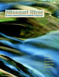
Assessment of Floodplain Wetlands of the Lower Missouri River
Using an EMAP Study Approach,
Phase II: Verification of Rapid Assessment Tools
Kansas Biological Survey Report No. 165
September 2010
by
Jason Koontz, Donald G. Huggins, Craig C. Freeman, and Debra S. Baker
Central Plains Center for BioAssessment
Kansas Biological Survey
University of Kansas
for
USEPA Region 7
Prepared in fulfillment of USEPA Award R7W0812 and KUCR Project 451000

Table of Contents
Abbreviations ..............................................................................................................................4
Executive Summary ....................................................................................................................5
Background .................................................................................................................................5
Introduction ................................................................................................................................6
Methods ......................................................................................................................................7
Site selection ...........................................................................................................................7
Field methods ..........................................................................................................................8
Macroinvertebrates ..................................................................................................................9
Disturbance Assessment ........................................................................................................ 10
The Assessment ................................................................................................................. 10
Wetland Attributes ............................................................................................................. 11
Reference Indicators .......................................................................................................... 12
Disturbance ........................................................................................................................ 13
Results ...................................................................................................................................... 14
Explanation of statistical analyses and graphical representations ............................................ 14
Floristic Quality Assessments ................................................................................................ 15
In situ water quality ............................................................................................................... 20
Depth measures ..................................................................................................................... 21
Nutrient Analyses .................................................................................................................. 22
Nitrogen ............................................................................................................................. 24
Phosphorus ........................................................................................................................ 26
Carbon ............................................................................................................................... 27
Herbicides ............................................................................................................................. 29
Comparisons between Phase I and II studies of the lower Missouri River floodplain wetlands .. 30
Introduction and Background Information ............................................................................. 30
Floristic Quality Assessment Results ..................................................................................... 31
Plant Richness - All Species ............................................................................................... 32
Plant Richness - Native Species ......................................................................................... 33
Spatial attributes .................................................................................................................... 34
Wetland area ...................................................................................................................... 34
Depth to Flood ................................................................................................................... 35
Mean Depth and Maximum Depth ..................................................................................... 36
Water quality ......................................................................................................................... 38
Dissolved oxygen ............................................................................................................... 38
Turbidity ............................................................................................................................ 38
Carbon ............................................................................................................................... 40
2 of 84

Nitrogen ............................................................................................................................. 41
Phosphorus ........................................................................................................................ 44
TN:TP ratio ........................................................................................................................ 45
Chlorophyll-a ..................................................................................................................... 46
Specific Conductance ......................................................................................................... 48
Herbicides .......................................................................................................................... 50
Resampled sites ..................................................................................................................... 52
Disturbance Assessment ........................................................................................................ 54
Macroinvertebrate MMI ........................................................................................................ 56
Metrics ............................................................................................................................... 56
a priori Groups and Metric Selection .................................................................................. 58
Metric Testing .................................................................................................................... 59
The Macroinvertebrate Multiple Metric Index (MMI) ........................................................ 66
MMI in Relation to Other Measures ................................................................................... 70
Differences in Wetland Types ............................................................................................ 71
Wetland Types and MMI Scores ........................................................................................ 72
MMI Result Conclusions ................................................................................................... 74
References ................................................................................................................................ 75
Appendix A. Goals and objectives of EPA Award R7W0812. .................................................. 78
Appendix B. Study sites for Phase II. ....................................................................................... 80
Appendix C. Laboratory measurements and analyses. .............................................................. 83
Appendix D. Disturbance assessment scoring form. ................................................................. 84
3 of 84

Abbreviations
AB – Aquatic beds
ANOVA – Analysis of Variance
AP – Agricultural Pesticides
BU – Burrower
Chl-a – Chlorophyll-a
CPCB – Central Plains Center for BioAssessment
CN – Clinger
DA – Disturbance Assessment
DEA – Desethylatrazine
DIA – Desisopropylatrazine
DOC – Dissolved Organic Carbon
DTF – Depth to Flood
EM – Emergent macrophyte beds
EMAP – Environmental Monitoring and Assessment Program
EPA – Environmental Protection Agency
EPT – Ephemeroptera, Plecoptera, and Trichoptera
ETO – Ephemeroptera, Trichoptera, and Odonata
FQA – Floristic Quality Assessment
FQI – Floristic Quality Index
FC – Filterer-Collector
GC – Gatherer-Collector
GIS – Geographic Information System
GPS – Global Positioning System
HM – Heavy Metal
IQR – Interquartile Range
KBS – Kansas Biological Survey
MIX – Wetlands with equally dominant AB, EM, and UB
MMI – Multiple Metric Index
MS – Microsoft
NCSS – Number Cruncher Statistical System
NOD – Nutrient and Oxygen Demanding chemicals
NTU – Nephelometric Turbidity Units
PA – Parasite
Pheo-a – Pheophytin-a
PI – Piercer
PL – Planktonic
POC – Persistent Organic Carbons
PR – Predator
RTV – Regional Tolerance Value
STDDEV – Standard deviation
STDERR – Standard error
SP – Sprawler
SSS – Suspended Solids and Sediments
TOC – Total Organic Carbon
UB – Unconsolidated beds
4 of 84

Executive Summary
This project sought to identify a number of Missouri River floodplain wetlands for monitoring
and assessment of wetland condition using several assessment tools developed in this and a
previous project entitled “Assessment of Floodplain Wetlands of the Lower Missouri River
Using an EMAP Study Approach”(www.cpcb.ku.edu/research/html/ReferenceWetlands.htm).
A number of randomly selected wetlands were identified using the probability-based sampling
design of the EMAP program (www.epa.gov/bioiweb1/statprimer/probability_based.html) and
monitored for four groups of attributes; water quality (e.g. dissolved oxygen, total phosphorus,
herbicides), floristic (native plant richness, percent adventives species), macroinvertebrate
community (taxa richness, sensitive species), and landscape (e.g. buffer condition, disturbance
assessment). A snapshot of the ecological condition of these wetlands were determined using
measures of various factors in the above groupings and these factors used to characterize the
random wetland population (see CDFs, descriptive statistics tables (Tables 3-7), and box plot
figures as examples). In addition a floodplain wetland database and series of GIS shape files of
various wetland and related attributes is available at the CPCB‟s website
(http://www.cpcb.ku.edu/research/html/wetland2.htm) that allow other wetland planners and
managers to access these data to assist in identify wetland condition and relationship that can
affect their management efforts.
In order to accomplish the first objective, the applicability and responses of both previously
determined assessment metrics (such as reference buffer condition, FQA metrics, field
disturbance assessments) and new metrics (this study‟s MMI and macroinvertebrate metrics)
were determined as part of this project. This effort produced a new macroinvertebrate
multimetric index (MMI) and series of metrics that can be used to quantify wetland disturbance
based on reference wetland scores. The disturbance assessment approach (DA) developed as par
to this and the prior floodplain wetland project was found to be useful as a Level II wetland
assessment tool and can be used by others in Region 7 to examine the possible level of
disturbance of individual wetlands occurring in large river floodplains. Lastly, comparisons of
reference and random population wetland conditions using project water quality, floristic and
macroinvertebrate metrics proved useful in identifying a continuum of conditions for these
wetlands from “least disturbed” to disturbed. The development of these tools and their
demonstrated value in determining possible wetland disturbances, quantifying biological and
water quality conditions related to disturbances, and the determination of “reference” conditions
(and wetlands) provides management organizations a new set of tools in developing wetland
plans for floodplain wetlands in EPA Region 7.
Background
In 2007 the Central Plains Center for BioAssessment (CPCB) at the Kansas Biological Survey
(KBS), University of Kansas, studied a set of 22 reference wetland sites located in the Missouri
River floodplain (Kriz et al. 2007). During that Phase I study, wetland assessment tools were
developed that could be useful for Level 1 (landscape assessment using a geographic information
system (GIS) and remote sensing) studies and could be applicable to Level 2 and Level 3 studies
(see Fennessy et al. 2004). This report describes a Phase II study in which we continued
development of the assessment tools by sampling and analyzing a series of abiotic and biotic
5 of 84

factors associated with 42 randomly selected wetlands in 2008 and 2009. The objectives of this
Phase II study of these randomly selected lower Missouri River floodplain wetlands were to 1)
obtain a “snapshot” of the ecological condition of the study population, 2) test the applicability
and responses of the previously developed wetland assessment metrics, and 3) compare
“reference” wetlands (from Phase I) with this random sample population of wetlands. Four
groups of attributes were examined for each study wetland: water quality, floristic,
macroinvertebrate community, and landscape. Analysis of relationships among buffer and
landscape attributes, water chemistry, and biological attributes are described.
Assessment data gathered for this population of 42 randomly selected wetlands were compared
against the reference sites studied in Phase I to identify baseline reference conditions for water
quality and benchmarks for determining wetland health. Project objectives are linked to EPA‟s
Strategic Plan, Goals 4.3.1.1, 4.3.1.3, and 4.3.2.1, by identifying and assessing critical wetlands,
developing rapid assessment tools, and providing baseline data, thus enhancing our ability to
track loss and degradation of wetland resources and identify opportunities for wetland protection
or restoration to support the “no overall net loss” goal of EPA‟s Strategic Plan. Specific project
goals are described in Appendix A.
Introduction
The floodplain ecosystems of the Missouri River basin have been severely impacted over the
course of U.S. history; this has been especially true since the completion of the six main-stem
dams built between 1930 and 1950 (Chipps et al. 2006). The transformation of natural prairies,
riverine areas, and wetlands to agricultural land via clearing, draining, and filling has destroyed
much of the wetland acreage once found there. The loss of wetland acreage is a continuous trend
with an increasing amount of disturbance due to urbanization and extension of rural areas
through the development of roads and other infrastructure (Dahl 2000). After 633,500 acres
were lost between 1986 and 1997, an estimated 100 million acres of freshwater wetlands
remained within the U.S. (Dahl 2000). Alterations to the Missouri River, including berms and
levees, have disrupted the connectivity between the river and remaining floodplain wetlands.
Wetland loss also is occurring due to natural succession caused by the changing course of the
river, however these natural processes are now constrained by human control of flooding.
Nevertheless, human disturbance has had great impacts on the Missouri River floodplain
wetlands and their capacity to provide crucial ecosystem services such as wildlife habitat,
nutrient cycling, carbon sequestration, and contaminant removal from upland and riverine
systems.
The biological integrity of the aquatic ecosystem has become an important component for
assessing wetland condition and quality. Aquatic macroinvertebrates respond to an assortment
of abiotic and biotic factors. Many wetland assessments use multiple tier approaches to quantify
wetland health and to identify perturbations that may cause degradation to a system. This study
was designed to assess the quality of wetlands in the lower Missouri River floodplain using
remote sensing technology, a rapid on-site landscape and hydrological assessment, a floristic
quality assessment, in situ water quality and nutrient measures, and benthic macroinvertebrate
collections. A multiple metric index (MMI) development approach was chosen to evaluate the
aquatic invertebrate community as a quantifiable measure of how these organisms respond to
6 of 84

other wetland parameters and assessment outcomes developed in this study. As an index of
biological integrity (IBI), the macroinvertebrate MMI was developed by scrutinizing the stressorresponse
relationships between the chemical and physical measures, and components of the
benthic macroinvertebrate community. Results of the macroinvertebrate MMI were consistent
with other studies using invertebrate metrics for assessing the biological integrity of aquatic
ecosystems when comparing the reference and random sample populations. The developed MMI
was then tested for congruency with the other assessment results, relationships to hydrological
connectivity, and internal wetland structural features that were evaluated. The macroinvertebrate
MMI responded significantly to observed physical and chemical anomalies, and provided insight
to dominant wetland features such as landscape, hydrology, water chemistry, and plant
communities, that influence wetland conditions.
Methods
Site selection
During Phase I (e.g. reference wetland identification, characterization, development of
assessment tools) of this two-part study, geospatial data from several sources were analyzed
using ArcView 3.3 and ArcGIS. From this a map was developed of all wetlands in the lower
Missouri River valley. We also developed a flooding model that identifies flood-prone areas
within the valley. NWI maps were merged into a single seamless data theme for the entire study
area, and a 500-year floodplain boundary was used to select wetlands within areas of interest.
Two classes of wetlands (as defined by Cowardin et al. 1979) were studied: lacustrine and nonwoody
palustrine.
Wetlands were filtered by size (i.e. surface acres) to identify those that meet our minimum size
criterion of 10 acres in area. Imposition of this wetland size criterion was done for four reasons.
First, it ensures a high likelihood of open water during spring to early summer. Second, larger
sites have a higher probability of being correctly classified in the NWI database. Third, larger
sites generally support higher levels of native biodiversity, more wetland functions, and greater
wildlife value. Fourth, bigger wetland area are more likely to be in public ownership and
therefore more likely to have been studied in the past.
For this Phase II study, from the population of wetlands meeting the location, class, and size
criteria, 400 were identified using EMAP selection protocols. From this population, 42 study
sites were selected randomly within a spatially hierarchical sampling framework called
Generalized Random Tessellation Stratified Designs (GRTS) (Figure 1). In GRTS, a hexagonal
grid is imposed on the map of the target population. The grid scale is adjusted to appropriate
levels of resolution. Grid elements (and sampling units) are then randomly selected using a
robust, selection algorithm. GRTS simultaneously provides true randomness, ensures spatial
balance across the landscape, and enables the user to control many parameters.
7 of 84

Figure 1. Map of the Lower Missouri River floodplain wetlands studied in Phase I and II. Phase
I studies focused on 22 candidate reference wetlands and their characterization. Phase II studies
focused on 42 randomly chosen wetlands that had open water and macroinvertebrate samples
Field methods
See the project Quality Assurance Project Plan (QAPP) for details of sampling methods
(http://www.cpcb.ku.edu/research/assets/PhaseIIwetlands/QAPP_wetlandsII.14Aug.pdf). The
disturbance assessment and the floristic quality assessment are composed of metrics (values that
represent qualitative aspects). Metrics from each study wetland were combined to produce a
score that estimated the wetland‟s condition with respect to the amount of disturbance or the
8 of 84

quality of plant community, respectively. The floristic quality index is only one component for
assessing the plant community in wetlands. Other factors, such as native wetland plant species
richness, may also indicate the condition of the wetlands health or quality to maintain diverse
communities of invertebrates and vertebrates, including amphibians, water fowl, and small
mammals. In situ water quality measures in this study consisted of mean values for water depth,
Secchi disk depth, water temperature, turbidity (NTU), conductivity (mS/cm), dissolved oxygen,
and pH. Water depth was measured with a surveyor‟s telescoping leveling rod to the nearest
centimeter. Water properties were measured with a Horiba U10 Water Quality Checker. One
liter samples were collected along three imaginary transect lines at right angles to a line
extending along the longest axis of the study wetland and combined in a 5-liter carboy as one
composite sample (Figure 2). Chemical laboratory analysis was conducted on composite water
samples for concentrations of chlorophyll-a, nitrates, nitrites, ammonia, total nitrogen, total
phosphorus, total and dissolved organic carbon (TOC and DOC), and six agriculturally applied
herbicides, including atrazine and its two major metabolites. Chlorophyll-a analysis was
conducted using fluorometric methods, nitrogen and phosphorus concentrations were determined
with inline digest flow injection analysis, TOC and DOC were measured with a Shimadzu TOC
analyzer, and herbicide concentrations were determined using Gas Chromatography/Mass
Spectrometry (see Appendix C for analytical and measurement methods). All water quality
analyses were conducted in CPCB‟s chemistry laboratories except the herbicides analyses, which
were performed at the University of Kansas‟s Chemistry Department laboratories.
Figure 2. Illustration of wetland survey layout. X = wetland centroid where GPS location was
recorded. A = long axis transect line. B = cross axis transect lines. C = composite water
sample. ● = in situ water quality measurement locations.
Macroinvertebrates
Macroinvertebrate sampling was conducted at four sites in the littoral zone of the major
vegetated habitat areas within each wetland. These zones were usually transitional areas
between open water and emergent macrophyte beds, more commonly referred to as „edge‟
habitat. At each zone, a kick and sweep method with a 500-micron D-frame aquatic net was
used to capture invertebrates in the benthos substrate. The surface of the benthos was disturbed
9 of 84

for 30 seconds with movement of the foot through the approximately top 10 centimeters of
substrate, while sweeping the net through the water column directly above the turbulence. The
contents of the aquatic net sample from each of the four zones were transferred from the net to a
one-liter Nalgene collection bottle to create a composite sample. To ensure proper preservation
of invertebrate collection, multiple bottles for each sample site were used with each sample
bottle filled to one-third the volume with collected substrate. Bottles were labeled and samples
were preserved in 10% buffered formalin with rose Bengal.
Macroinvertebrate samples were relinquished to the custody of the CPCB macroinvertebrate lab,
rinsed of field fixative, and sorted to a 500 organism count according to the USEPA EMAP
methods (USEPA 1995, USEPA 2004), explained in the Standard Operating Procedure (SOP) of
the CPCB at the KBS (Blackwood 2007). Specimens were identified to the genus level for most
taxonomic groups when possible (Blackwood 2007). Data were recorded on data sheets and then
entered into a Microsoft Access relational database.
Macroinvertebrate data containing taxonomic names and specimen counts were linked to an
integrated taxonomic information system (ITIS) (www.itis.gov/index.html) data table, and fields
containing higher taxonomic groups were created (Phylum, Class, Order, etc.). Errors in
nomenclature were identified and corrected before further field creation and classification
commenced. In ECOMEAS software (Slater 1985), total taxon richness, Shannon‟s diversity
index, and other diversity indices were computed for each sample. Feeding guilds, habitat
behavior, tolerance, and sensitivity values were added to the macroinvertebrate database
(Barbour et al. 1999, Huggins and Moffett 1988). Taxa without this information were updated
from the aquatic insect identification and ecology literature (Smith 2001, Thorp and Covich
2001, Merritt and Cummings 2008). Additional metrics were calculated from this information
and all macroinvertebrate metrics exported along with water quality, herbicide, floristic, and
disturbance variables to the Number Cruncher Statistical System (NCSS) (Hintze 2004) for
statistical analysis.
Disturbance Assessment
The Assessment
After considering several reviews of wetland rapid assessment methods (Fennessy et al. 2004,
Fennessy et al. 2007, Innis et al. 2000), the Ohio Rapid Assessment Method (Mack 2001) and
the California Rapid Assessment Method (Sutula et al. 2006) were used as models in designing
the Missouri River Floodplain Wetland Disturbance Assessment. While the California and Ohio
methods attempt to provide a more or less comprehensive evaluation of wetland rapid
assessment parameters, the disturbance assessment developed for this study focused on Wetland
Attributes, Reference Indicators, and Disturbance (Table 1). Wetland Attributes are used to
score how able the wetland is to deal with disturbance (or how it is currently dealing with it).
Reference Indicators are those wetland characteristics and conditions most often associated with
least impacted or minimally impacted wetlands. Other indicators might include public use
restrictions, protective regulations associated with some wetland areas and other factors that
might be protective of wetland structure and function. Disturbance is defined as evident
physical perturbations or known observable impairments that may occur as a result of them, such
as excessive sedimentation and/or altered hydrology. Some overlap between assessment metrics
10 of 84

was inevitable, but care was taken to avoid redundancies in scoring. Metrics dealing directly
with the classification scheme used in this study (i.e. depth and the temporal dimension of
inundation) were also left out. Finally, metrics pertaining to the water and floristic quality
response variables measured in the field that deal with known ecological impacts of disturbance
were limited so as not to affect adversely a comparison with data from a Floristic Quality
Assessment.
The resulting assessment method is advantageous in the sense that it is a subjective scoring
process in which the user is evaluating human impacts without being asked to make specific
judgments about the more technical aspects of wetland ecological integrity. Though the three
sections in the disturbance assessment are meant to be used together to estimate an overall score
for a wetland or specific area within a wetland complex. In addition attributes and scoring
within each of the three sections can be examine individually to more specifically assess or
describe certain wetland characteristics or trends in wetland condition.
Table 1. Assessment parameters used in quantifying disturbance. Wetland attributes are scored
up to 3 points each, and reference and disturbance parameters ±1 point. See Appendix D for
field sheet used in scoring.
Wetland Attributes
Three wetland size classes (50 acres) were selected based on the
range of surface areas for individual wetlands and wetland complexes in the lower Missouri
River floodplain and the findings of other rapid assessment methods (e.g., the Ohio Rapid
Assessment Method) gauged as appropriately “large” wetlands.
Natural buffer width or buffer thickness was an important metric according to several published
assessment methods. Natural buffers are thought to provide protection against local
disturbances.
11 of 84

Surrounding land use is defined as intensive, recovering, undisturbed, or a mixture of intensive
and undisturbed (scored the same as “recovering” landscape). Row crops, grazed pasture,
residential areas, and/or industrial complexes that are adjacent to the study area were considered
intensive uses. Natural buffer should be considered part of the surrounding land in the
„undisturbed‟ category.
Hydrology can be an indicator of wetland class and vary independently of human disturbance.
However, in the context of assessing human disturbance and in some respect functionality in the
landscape (in terms of connectivity), different hydrological variables were scored according to
potential and actual water source(s) for individual wetlands. Historically, floodplain wetlands
probably received water; 1) directly as a result of local precipitation events (e.g. rainfall and
localized runoff), 2) as groundwater from the shallow water table of the floodplain, and 3) from
flood waters as a result of the historical hydrologic regimes. Wetlands develop rapidly with a
continual (or seasonal) inflow of river water (or overland flow), which maintains steady
propagule/organism inflow and allows for mixing of basins during floods, a process known as
„self-design‟ (Mitsch et al. 1998). Since the most natural functional condition for floodplain
wetlands would include their filling and flushing by floodwaters associated with natural
hydrological events within the river basin, the assessment of the degree of hydrological
disturbance must include an estimate of “disconnection” of the wetland from the river system.
While assessment of all factors (e.g. number of dams, amount of channelization and levees) that
may affect the hydrological connection between the river and wetland is difficult due to scale
issue an attempt was made to estimate and score natural hydrological conditions highest, wherein
less natural sources, such as storm water drains or channelized ditches receive an intermediate
and low scores.
Vegetation coverage below 20% was thought to be indicative of a disturbed wetland or a wetland
that is more venerable to perturbations. Coverage of over 70% often reduces the amount of open
water to vegetation “edge” and the potential for habitat diversity, so receives an intermediate
score. Finally, 40-70% coverage was thought to be ideal for floodplain wetlands because a
moderate amount of vegetation coverage suggests a high occurrence of edge habitat between
open water and vegetated areas, providing for a diversity of habitats.
Reference Indicators
Indicators of reference conditions refer to the absence of human disturbance within the wetland.
Metrics that reflect undisturbed ecological condition can be combined for a condition score used
to track the status of a site. Reference indicators are a combination of factors that impede and
control human disturbance or indicate the presence of valuable wetland features or “value-added
metrics” (Fennessy et al. 2007). The inclusion of reference indicators was necessary to facilitate
the inclusion of factors that were not numerically quantifiable like those evaluated in the
Wetland Attributes section, but were better evaluated by their presence or absence.
Protected wetlands deter certain types of human disturbance over time, thereby increasing the
probability that the wetland experiences relatively little disturbance (except for management,
which is discussed in the next section).
12 of 84

Evidence that waterfowl and/or amphibians are present or would be present during the migratory
season, suggests the wetland is capable of providing wildlife habitat, including food and nesting
cover.
Endangered or Threatened Species warrant further protection of the area under federal laws and
would thus generally discourage disturbance.
Interspersion (Mack 2001) refers to natural non-uniformity in wetland habitat design. Some
native wetland species require multiple habitat-types. If these habitat-types are not in close
proximity to one another, or interspersed throughout the wetland area, then it may be difficult for
such species to survive. The assumption is that between two wetlands of the same size and with
the same proportions of open-water to vegetated habitat, the one exhibiting the greatest
interspersion of habitats likely will support greater native wetland biodiversity and will be more
similar to a „reference‟ state.
Connectivity refers to a wetland‟s functional and structural connection to other landscape and
hydrologic features. Features that disrupt connectivity, such as river or stream impoundments,
levees, berms, or other water structures, can be easily identified on a local level and indicate
disruptions to historical hydrologic regimes. It is more difficult to assess broad-scale and
cumulative hydrological impacts to floodplain wetlands since at some scale nearly all floodplains
and riverine systems have become hydrologically altered to some degree. This assumes most
floodplain wetlands were originally connected to the river or that water was able to cycle
between these systems intermittently.
Disturbance
Metrics that indicate human disturbances known to degrade wetland health are listed in this
section of the Disturbance Assessment. For each disturbance a point is subtracted. If the
disturbance is unusually severe or at a high rate of occurrence, then more than one point can be
subtracted.
Sedimentation is a natural process for wetlands in the Missouri River floodplain, however
modern land use changes that affect the spatial and temporal extent of permanent ground cover
can accelerate soil loss and increased sedimentation (observed as plumes or fresh deposits within
wetlands) that dramatically affect the structure and function of wetlands. Scoring the extent of
wetland sedimentation is not dependant on the identification of anthropogenic or natural causes.
Upland soil disturbance or tillage in the immediate area drained by the wetland is scored
separately as a local disturbance that demonstrates the potential for excessive sedimentation,
although it may not be observable at the time of evaluation.
The presence of cattle is not considered a natural occurrence, even in circumstances where the
cattle graze the wetland periodically throughout the year.
Excessive algae usually suggest an imbalance within an aquatic ecosystem (i.e. excessive
nutrients or eutrophication). Regardless of whether the cause is fertilizer run-off, sediment
resuspension, or cattle, the presence of excessive algae can impede the growth of
aquatic/emergent plant life and threatens the survival of some aquatic organisms.
13 of 84

Wetland surface area is comprised of over 25% invasive species. Invasive plant species are
themselves a disturbance and an indicator of degraded wetland conditions (e.g. hydrological
alterations, soil disturbance) that favored their growth over native species.
Steep shore relief is a common occurrence in created wetlands that were constructed during the
last few decades of the 20th century. Examples would include “barrow” pits from road
construction, farm ponds, or natural wetlands that were dredged to reduce the littoral zone.
Some of these wetlands exhibit a uniform depth and, although they may cover areas of hundreds
or thousands of acres, they may exhibit little shore relief. In nature, a high shore length to
surface area ratio and gradual relief in littoral zones generally characterize floodplain wetlands in
the Midwestern US. The structural uniformity of some created and altered wetland systems may
favor invasive species and decrease biodiversity.
Hydrologic alterations that contribute to “disconnection” of the wetland from the historical flow
regime of the river are differentiated from alterations that contribute to their historic connectivity
with the riverine system.
Management for specific purposes, such as hunting, fishing, or wildlife preservation may result
in systems that are broadly impaired and do not fully support other wetland uses or functions.
Management practices can be observed at particular wetland sites and their objectives confirmed
by conversations with the landowners or designated managers.
Results
Explanation of statistical analyses and graphical representations
Comparisons between study phases, ecoregions, major wetland classes, and vegetative types
were performed on FQA, disturbance assessments, water quality parameters, and
macroinvertebrate metrics with ANOVA means analysis and Tukey-Kramer multiple
comparison t-tests when sample populations were found to be normally distributed or when
normal distribution could be obtained via log transformation. When ANOVA assumptions of
distribution could not be assumed either due to number (n < 5) or distribution (i.e. skew, log
factor, kurtosis), Kruskal-Wallace non-parametric variance analysis and normal Z-tests were
performed. All statistical significance was measured at 95% confidence (α = 0.05) with Kruskal-
Wallace p values corrected for ties. Relationships between parameters were investigated with
Pearson auto-correlations matrix having significant p values (≤ 0.05). Correlation coefficients
and p values are reported when significance is found. Relationships were further scrutinized
with robust linear regression routines that accommodate discrepancies associated with outlier
data. Adjusted R 2 values and significant p values associated with linear regression t–tests are
reported when statistically significant values were obtained. When statistical significance is not
obtained, no value of p, R 2 , or Pearson correlation coefficient is reported, and it can be assumed
the level of significance was not achieved (p > 0.05) and the relationship was not substantial.
Box plot representations are used extensively throughout the text because range, distribution, and
identification of moderate and extreme outliers become readily apparent. Box area represents
inner quartile range (IQR), while “whiskers” represent the upper observation that is less than or
equal to the 75 th percentile plus 1.5 times the IQR upper value and the lower observation that is
greater than or equal to the 25 th percentile minus 1.5 time the IQR lower value.
14 of 84

Floristic Quality Assessments
Floristic Quality Assessments were conducted for all 42 sites visited during the 2008 and 2009
seasons; mean and median values of plant community metrics and final Floristic Quality Indices
(FQI) are reported in Table 2. Only mean values and variance in mean conservatism were found
to be significantly different between sample populations of the Western Corn Belt Plains (n = 21)
and Central Irregular Plains (n = 16) ecoregions based on ANOVA evaluation and Tukey-
Kramer multiple comparison tests. The mean value for the Interior River Valleys and Hills
sample population (n = 5) fell between the other two ecoregion sample populations, with mean
value of mean conservatism of native plant species for the Central Irregular Plains, Interior River
Valleys and Hills, and Western Corn Belt Plains regions being 4.58, 4.08, and 3.64, respectively.
Mean conservatism for all plant species mean ecoregion values were slightly lower than that of
native plant species but maintained the same hierarchy (Table 2, Figure 3).
Table 2. Descriptive statistics for Florist Quality Assessment metrics of the random population
of wetlands in the floodplain of the Missouri River.
Metric Count Mean STDDEV Median Min Max
FQI All 42 17.18 4.40 16.57 9.43 26.11
FQI Natives 42 18.17 4.31 17.69 11.09 27.14
Richness All 42 27.12 15.14 25.00 5.00 66.00
Richness Native 42 23.76 12.99 22.00 5.00 55.00
Percent Adventive 42 11.20 8.13 10.00 0.00 30.43
Mean Conservatism All 42 3.64 1.07 3.63 1.70 6.00
Mean Conservatism Natives 42 4.05 0.97 4.10 2.16 6.00
Mean Conservatism Mean Values
5.0
4.8
4.6
4.4
4.2
4.0
3.8
3.6
3.4
3.2
3.0
Central
Irregular
Interior
River
Ecoregion
Figure 3. Error bar chart of ecoregional means of mean conservatism values for plant richness of
all and native species.
15 of 84
Western
Corn Belt

Though the majority of wetland polygons surveyed were found to be palustrine systems based on
Cowardin's 2-meter depth criterion, wetlands were assigned dummy variables that indicating
their dominant hydrological influence. Lacustrine systems in this survey were of two types:
polygons identified as lakes by the NWI dataset and having dominant aquatic plant establishment
or polygons that were littoral zones of lakes with wetland features. Palustrine systems were
either identified by NWI as freshwater emergent wetlands or lakes, yet had consistently shallow
depths and were dominated by emergent macrophytes. Riverine systems were those wetlands
identified by field observation and GIS mapping that were backwaters and sloughs having
continuous connectivity or frequent connectivity with the Missouri River. Significant
differences in FQI, plant richness, mean conservatism, and percent adventive species were
identified in ANOVA evaluation based on this assigned wetland classes. The palustrine sample
population maintained statistically significant higher mean FQI All and FQI Native scores over
the riverine sample population. The palustrine sample population also had significantly higher
plant richness for all and native species. The riverine sample population had higher mean
percent adventives than the lacustrine sites with palustrine sites falling somewhere between and
similar to both lacustrine and riverine types. Finally, lacustrine types had significantly higher
mean values of mean conservatism for all and native species. All mean values and variance were
significant for the relationships between FQA metrics and wetland hydrological classes
mentioned above based on ANOVA and Tukey-Kramer multiple comparison tests (p < 0.05,
Table 3-5, Figure 4-7).
Table 3. Descriptive statistics for Floristic Quality Index (FQI) scores for wetland classes:
lacustrine, palustrine, and riverine.
FQI ALL
FQI NATIVE
Lacustrine Palustrine Riverine
Count 15 21 6
Mean 16.62 18.85 12.74
Median 16.36 18.57 10.73
StdDev 3.6 4.2 4.01
Min 11.4 11.67 9.43
Max 22.39 26.11 19.45
Mean 17.22 20.04 14.01
Median 17.03 20.23 11.98
StdDev 3.57 4 3.87
Min 12.56 13.15 11.09
Max 23.7 27.14 20.43
16 of 84

FQAI ALL
30
25
20
15
10
5
0
Figure 4. Box plots of floristic quality index scores (FQAI) for: (a) all plant species and (b)
native plant species.
Table 4. Descriptive statistics of plant richness among lacustrine, palustrine, and riverine
wetland classes for both native plants and the entire community of plants.
RICHNESS
ALL
RICHNESS
NATIVES
a
Lacustrine Palustrine Riverine
Wetland Class
FQAI NATIVES
30
25
20
15
10
Lacustrine Palustrine Riverine
Count 15 21 6
Mean 14.4 37.43 22.83
Median 13 36 22.5
StdDev 6.05 13.44 10.07
Min 5 16 7
Max 27 66 35
Mean 13.4 32.57 18.83
Median 12 30 17.5
StdDev 5.85 11.44 9.33
Min 5 16 6
Max 27 55 30
5
0
17 of 84
Lacustrine Palustrine Riverine
Wetland Class
b

PLANT RICHNESS ALL
80
60
40
20
0
Lacustrine Palustrine Riverine
Wetland Class
Figure 5. Box plots showing distribution of plant richness values for: (a) all and (b) native
species among the lacustrine, palustrine, and riverine wetland classes.
Table 5. Descriptive statistics of selected FQI metrics (percent adventive species and mean
conservatism for all and native species) among lacustrine, palustrine, and riverine wetland
classes.
PERCENT
ADVENTIVE
MEAN
CONSERVATI
SM ALL
MEAN
CONSERVATI
SM NATIVES
a
PLANT RICHNESS NATIVES
80
60
40
20
Lacustrine Palustrine Riverine
Count 15 21 6
Mean 7.04 12.14 18.3
Median 7.69 10 14.29
StdDev 6.64 7.56 8.61
Min 0 0 9.38
Max 18.18 27.08 30.43
Mean 4.54 3.23 2.8
Median 4.54 3.45 2.5
StdDev 0.77 0.9 0.76
Min 2.76 1.7 2.13
Max 6 4.88 4
Mean 4.87 3.64 3.4
0
Median 4.94 3.56 3.11
StdDev 0.68 0.83 0.72
Min 3.36 2.16 2.68
Max 6 4.88 4.67
18 of 84
b
Lacustrine Palustrine Riverine
Wetland Class

MEAN CONSERVATISM ALL
6
5
4
3
2
1
0
Figure 6. Box plots of mean conservatism values for: (a) all and (b) native species among
lacustrine, palustrine, and riverine.
PERCENT ADVENTIVES
Lacustrine Palustrine Riverine
Wetland Class
35
30
25
20
15
10
5
0
a 6
b
Figure 7. Box plots of percent adventive values among lacustrine, palustrine, and riverine
wetland classes.
MEAN CONSERVATISM NATIVES
In addition to class, wetlands were identified as having three dominant plant community
structures and were classified according to the type of vegetated conditions observed. Aquatic
beds (AB) were wetlands with open waters zones commonly inhabited by obligate aquatic
submergent and emergent hydrophytes. Unconsolidated beds (UB) were wetlands that had open
water zones, but were more frequently observed having little to no hydrophytes or fringe flora
such as geophytes (i.e. cattail, bulrush, etc). Emergent macrophyte beds (EM) were commonly
very shallow palustrine sites with dense stands of cattail, bulrush, reed canary grass (Phragmites
sp.), and other facultative wetland plants. Wetlands that were found to have all three types
5
4
3
2
1
0
19 of 84
Lacustrine Palustrine Riverine
Wetland Class
Lacustrine Palustrine Riverine
Wetland Class

equally dominant were classified as a mixed type (MIX). This is further discussed in the
comparison of Phase I and Phase II results.
In situ water quality
In situ water quality measures were collected at 38 of the 42 sites visited. Data collected
included depth measurements and water chemistry readings from the Horiba U10 water quality
checker including: water temperature, dissolved oxygen, mean pH, and mean turbidity (Table 6).
Significant differences among wetland classes were not observed for any of the water chemistry
metrics for the wetland population. However, log-transformed mean conductivity mean values
were significantly (p < 0.000) lower for the wetland population of the Central Irregular Plains
ecoregion than both the Western Corn Belt Plains and the Interior River Valleys and Hills
ecoregions (Figure 8).
Table 6. Descriptive statistics of random population in situ water chemistry measures.
Parameter
Mean depth
m
Maximum
depth m
Mean Secchi
depth m
Mean
temperature C
Mean
dissolved
oxygen
Count
Mean
Standard
dev
Standard
error
20 of 84
Min
Max
Median
25th
percentile
75th
percentile
38 0.63 0.43 0.07 0.11 2.08 0.51 0.35 0.81
38 1.06 0.82 0.13 0.2 4.2 0.82 0.49 1.29
38 0.43 0.46 0.08 0.08 2.82 0.31 0.18 0.6
38 27.06 2.78 0.45 20.4 33.5 26.95 25.48 28.63
38 6.19 3.15 0.51 0.38 12 5.93 3.48 9.02
Mean pH 38 7.77 0.78 0.13 5.59 9.53 7.61 7.33 8.26
Mean
turbidity NTU
Mean
conductivity
mS/cm
38 67.68 60.32 9.79 3 242 55 17.75 110
38 0.31 0.17 0.03 0.07 0.86 0.28 0.22 0.35

Mean Conductivity mS/cm
0.6
0.5
0.4
0.3
0.2
0.1
0.0
40 47 72
Ecoregion
Figure 8. Error bar chart of ecoregional means of mean conductivity values: 40 - Central
Irregular Plains, 47 - Western Corn Belt Plains, and 72 - Interior River Valleys and Hills. Error
bars are measures of standard error.
Mean value for the mean conductivity measures in the Central Irregular Plains ecoregion was
0.205 mS/cm, well below the values found in the Western Corn Belt Plain (0.342 mS/cm) and
the Interior River Valleys and Hills (0.307 mS/cm). Median values for the ecoregions were
similarly significantly different when Kruskal-Wallace non-parametric medians test was
performed. Many significant relationships between the mean conductivity and other assessment
metrics were observed and will be discussed later.
Depth measures
Mean and maximum depth measures for the Phase II samples (n = 38) were not normally
distributed thus log transformation of the depth values was necessary to perform the ANOVA‟s
to examine regional and class differences (Figure 9). Significant differences in mean and
maximum depths were not observed among ecoregions. When major hydrological system
classes were analyzed, log means and variance for the lacustrine sample population (n = 15) were
significantly higher in mean and maximum depths than the palustrine sites (n = 18) for both
measures and higher in mean depth than the riverine sample population (n = 5). Secchi depths
were also observed as being statistically higher in means among the lacustrine than both
palustrine and riverine samples.
21 of 84

Number of Samples
Number of Samples
15
10
5
0
0 1 2 3
30
20
10
Mean Depth in Meters
0
0 1 2 3
Mean Secchi Depth in Meters
Figure 9. Random (Phase II) sample population distribution represented by frequency
histograms of: (a) mean depth, (b) maximum depth, (c) Secchi depth, and (d) error bar chart of
all in situ depth measures. Error bars are measures of one standard error.
Nutrient Analyses
Many of the analyzed nutrients exhibited broad ranges and extreme values (
Number of Samples
20
a b
c
15
10
5
22 of 84
0
0 1 2 3 4 5
Maximum Depth in Meters
d

Table 7). The wide range of values reflects the large amount of variability observed across the
lower Missouri River floodplain wetlands. Evaluation of the various nutrient fractions and totals
can give us an idea of the primary productivity and nutrient cycling in the sample population.
23 of 84

Table 7. Descriptive statistics of nutrient measures for Phase II wetland water samples.
Nutrient Measure Count Mean Median STDEV Min Max
NO3 + NO2 mg N/L 38 0.03 0.01 0.03 0.01 0.13
NO2 mg N/L 38 0.01 0.01 0.00 0.01 0.02
NH3 µg N/L 38 85.01 48.95 115.95 18.90 555.00
Total N mg N/L 38 1.14 1.07 0.48 0.39 2.91
Dissolved N mg N/L 38 0.11 0.07 0.12 0.02 0.56
PO4 µg P/L 38 171.41 53.55 427.28 6.90 2630.00
Total P µg P/L 38 414.37 264.50 606.83 16.30 3710.00
Avail N:Avail P 38 3.04 1.21 5.44 0.05 29.63
TN:TP 38 5.34 4.19 4.79 0.48 23.93
Chlorophyll-a µg/L 38 30.68 24.47 30.99 0.70 171.83
Pheophytin a µg/L 38 12.38 10.17 10.96 0.71 65.41
TOC mg/L 38 10.54 9.80 3.81 5.60 20.74
DOC mg/L 38 9.23 8.75 2.98 5.40 17.93
Nitrogen
Measures of ammonia, nitrates, and nitrites were similar for all three major classes of wetlands
and all three ecoregions when ANOVA and Kruskal-Wallace non-parametric means analysis
were performed. Total nitrogen was almost significantly different between palustrine (1.34
mg/L) and both lacustrine (0.97 mg/L) and riverine (0.91 mg/L) classes (Figure 10-11). No
significant difference was found with Kruskal-Wallace non-parametric medians analysis and the
Tukey-Kramer multiple comparison tests. It was assumed that organic nitrogen component
could theoretically be obtained by subtracting all dissolved available nitrogen fractions from the
total nitrogen concentration value. Total nitrogen appeared to be comprised mostly of the
organic nitrogen fraction with little available dissolved nitrogen compounds. This may reflect
the overall high productivity that is generally associated with wetland ability to assimilate
external and internal nitrogen sources into biomass. This concept is reinforced by the observed
elevated concentrations in the palustrine wetlands which generally had higher plant richness and
greater densities of standing emergent macrophytes. However, some effects of concentration
over dilution may account for the variability in nitrogen concentrations.
24 of 84

Nitrogen - N mg/L
Total Nitrogen mg-N/L
10
1
.1
Lacustrine Palustrine Riverine
Wetland Class
Figure 10. Box plots of total nitrogen concentrations among lacustrine, palustrine, and riverine
classes in log scale.
3.0
2.0
1.0
0.0
7475
7463
Total N Organic N
Figure 11. Box plots of measure total and calculated organic nitrogen for random population of
Phase II study. Sites 7475 and 7463 were both emergent palustrine sites with very shallow mean
and maximum depths. Site 7475 (French Bottoms) was densely covered with reed canary grass
7475
7463
25 of 84

Phosphorus - P mg/L
with small intermittent pools having large amounts of detritus. 7463, located in the Swan Lake
complex also had significant detrital matter, but was dominated by cattail and bulrush. In the
Swan Lake site was edged with by a deeper pool allowing the establishment of some aquatic
plants.
Phosphorus
Most of the total phosphorus in these wetlands appeared to be organic phosphorus (Figure 12).
Median values for all forms of phosphorus were around 0.1 to 0.2 mg/L of P. However, total and
organic phosphorus levels in some wetlands were well above 1000 ug/L.
4.0
3.0
2.0
1.0
0.0
7460
7438
7461
7460
7463
7461
7438
Ortho P Total P Organic P
Figure 12. Box plots showing range of phosphorus values and moderate and extreme outliers
among the random population. Ortho P is orthophosphate.
Wetland groups created by aggregating wetlands into ecoregion and hydrological classes shared
similar log mean and median values among the nutrient measures of nitrogen and phosphorus.
Nitrogen to phosphorus ratios were also similar among these groups, though more outliers were
observed in the N:P groupings (Figure 13).
26 of 84
7460
7463
7461

N:P ratio
30.0
24.0
18.0
12.0
6.0
0.0
7454
7470
7453
7457
7444
Available N:P Total N:P
Figure 13. Box plots of nitrogen to phosphorus ratios, moderate, and extreme outliers among the
random population.
Carbon
Unlike nitrogen and phosphorus, measures of variance of total organic carbon (TOC) and
dissolved organic carbon (DOC) were found to be significantly higher in palustrine sites which
had a wider range of values than lacustrine or riverine sites (Figure 14). Tukey-Kramer multiple
comparison of mean values among classes revealed no significant differences. Medians test of
data did not identify significant variance or differences in median values for TOC or DOC. The
dissolved organic carbon makes up a considerable amount of the total water column carbon
measure, approximately 88%, indicating that carbon was not incorporated in sestonic organisms
and is in considerable surplus concentrations in these wetlands.
7457
7470
7437
7454
7474
27 of 84

Figure 14. Error bar plots of total and dissolved organic carbon concentration means among the
major wetland classes. Error bars are one standard error.
Normality tests of the chlorophyll-a and pheophytin-a data revealed that some samples were
significantly different than the rest of the population (Figure 15). Attempts to achieve normal
distribution via log transformation failed, thus data were analyzed for differences among
ecoregions and classes using the Kruskal-Wallace non-parametric medians test instead of the
ANOVA. The lacustrine sample population was determined to be significantly higher in median
chlorophyll-a concentrations than the palustrine population (Figure 16). The riverine population
shared ranges in variance with the other classes and the median value was similar to the others.
Number of Samples
20
15
10
5
20
a b
0
0 50 100 150 200
Chlorophyll a ug/L
Number of Samples
Figure 15. Frequency histograms showing sample distributions based on concentration of: (a)
chlorophyll-a and (b) pheophytin-a.
15
10
5
28 of 84
0
0 10 20 30 40 50 60 70 80
Pheophytin a ug/L

Chlorophyll a ug/L
200
180
160
140
120
100
80
60
40
20
0
Lacustrine Palustrine Riverine
Wetland Class
Figure 16. Box plots showing distribution of chlorophyll-a values for the lacustrine, palustrine,
and riverine wetland classes.
Herbicides
Atrazine was found more frequently and typically in higher concentrations than all other
herbicides. Atrazine metabolites (i.e. DIA and DEA) were often found at higher levels than the
parent compound and median values for these metabolites exceeded the median for atrazine itself
(Figure 17). No significant differences in concentrations or number of herbicides detected were
found among wetland populations within ecoregion or hydrological class Most sites had
measurable concentrations of six to seven of the eight herbicide analytes investigated. Simazine
concentrations were typically the lowest for all herbicides detected in this study (Figure 17).
29 of 84

Herbicide Concentration ug/L
10
1
.1
.01
DIA
Figure 17. Box plots of herbicide concentrations for Phase II samples.
DEA
Simazine
Comparisons between Phase I and II studies of the lower Missouri River floodplain
wetlands
Introduction and Background Information
Before comparing results of both of our studies of the floodplain wetlands of the lower Missouri
River some preliminary information is necessary. While we have referred to each of these
studies as Phase I (see Kriz et al. 2007) and Phase II (this report) for reporting clarity, it is more
accurate to refer to these two studies as reference and random population studies. The following
section is meant to provide, in part, an assessment of the tools we developed in these studies as
well as an assessment of the relative impairment of the randomly selected wetland population
based on reference conditions identified in Phase I.
One of the conclusions of the reference wetland study (i.e. Phase I) was three of the 18 reference
candidates (sites 7108, 7115, and 7116) were not of reference quality based upon their status as
created or restored wetlands and their floristic quality assessment metrics. However, current
evaluation indicated sites 7115 and 7116 had water quality and macroinvertebrate metric values
that were within the range of the Phase I reference population and that site 7108 was an extreme
outlier based on most water quality parameters, the floristic quality assessment, and
macroinvertebrate data. Hence, site 7108 was excluded from our comparison studies and sites
7115 and 7116 were considered reference wetlands. In many analyses the numbers of samples
(n) changed since not all sites had open water or an established macroinvertebrate community.
All sites (n=64) were assessed for floristic quality (i.e. 21 reference candidates and 42 randomly
selected wetlands). The final number of wetlands assessed using the developed Disturbance
Assessment was 18 reference and 42 random. Water quality data was available for 17 and 38
Atrazine
30 of 84
Metribuzin
Herbicides
Alachlor
Metolachlor
Cyanazine

wetlands, respectively. Macroinvertebrate collections were obtained from 54 sites, but the
exclusion of one outlier (site 7108) reduced the number to 53, with 16 samples from Phase I and
37 samples from Phase II. Because disturbance assessment data were used in the
macroinvertebrate selection process in developing a multiple metric index, one Phase I sample
(7107) was excluded during the MMI development process because this information was not
available. Because disturbance assessment information was used in development of the multiple
metric index (MMI), only 52 sites were used in developing the MMI but all 54 samples were
scored.
Floristic Quality Assessment Results
No significant differences were found between Phase I and Phase II sample populations when
ANOVA and Tukey-Kramer multiple comparison test were performed on the FQI and Native
plant FQI scores. However, significant differences (p = 0.001) in variance and mean total
richness and native richness were found between the two study groups. Total plant richness
mean value for reference sites was 41.05 (STDERR = 14.39) and 3.14 (STDERR = 2.34) for the
random sites. Native plant richness mean value for reference sites was 36.10 (STDERR = 2.68)
and 23.76 (STDERR = 2.00) for the random sites. Mean conservatism was also found to be
significantly different between reference and random, with 3.64 (STDERR = 0.17) for the
random population and 3.07 (STDERR = 0.17) for the reference population. A similar trend was
seen in the measure of native mean conservatism where the random population had a
significantly (p = 0.014) higher sample mean (4.05, STDERR = 0.15) than the reference
population (3.44, STDERR = 0.16). Mean percent adventive species values were not
significantly different between the two wetland populations. Further evaluation efforts in higher
order delineation of sites should consider these groups separately.
ANOVA and Tukey-Kramer multiple comparison tests were performed using all study sites to
examine possible differences associated with sample year. In the random population, mean FQI
was statistically higher (p = 0.04) in 2009 (n = 10, mean FQI = 19.65, STDERR = 1.33) than in
2008 (n = 32, mean FQI = 16.41). No significant differences in FQI were found between 2005
and 2009. ANOVA testing of FQI scores for 2005 and 2008 samples showed significant yearly
differences (p = 0.04) in FQI values. When all years were compared again using one-way
ANOVA and Tukey-Kramer comparison tests, significant yearly differences were again noted (p
= 0.03), though the post hoc comparison test did not clearly indicate group separations. ANOVA
test using only the randomly selected wetland data indicated that the mean Native FQI values
were significantly different (p = 0.02) between 2008 (17.34, STDERR = 0.72) and 2009 (20.83,
STDERR = 1.29). When 2005 and 2008 were evaluated without 2009, significant yearly
differences in were found with 2005 having a mean value of 19.99 (STDERR = 0.9); but when
2008 was excluded from analysis, 2005 and 2009 values were not significantly different from
each other (p = 0.62). This further suggests that 2009 plant community samples were similar to
those collected in 2005. It remains unclear if yearly conditions affected the FQI metric or if
differences were merely serendipity. Overall, the wetlands in both study phases appear to exist
on a continuum of floristic conditions as indicated by the overlapping FQI scores between and
among collection years.
The CDFs for both the reference and random wetland groups were similar, but the CDF for
reference wetlands indicated that most all of scores were above those of the random population
31 of 84

(Figure 19). This supports the contention that these groups are distinctly different from each
other floristically.
FQAI Score
24
22
20
18
16
14
12
10
8
6
4
2
0
a b
Figure 18. Mean error bar plots of florist quality assessment index scores for: (a) all species and
(b) native species.
CDF
2005 2008 2009
Year
100
90
80
70
60
50
40
30
20
10
0
Native Plants FQAI Score
Figure 19. Cumulative distribution frequency (CDF) of FQI scores for reference and random
populations of wetlands.
24
22
20
18
16
14
12
10
8
6
4
2
0
Plant Richness - All Species
Plant richness was significantly different (p = 0.001) among wetlands collected in each of the
three study seasons. When all years were compared, 2005 had significantly higher mean plant
richness value (41.05, STDERR = 3.14) than 2008 (24.91, STDERR = 2.61). When study Phase
II was examined alone, no significant differences (p=0.09) were found between 2008 and 2009,
with 2009 having a mean plant richness value of 34.2 (STDERR = 4.67). Exclusion of 2008
32 of 84
2005 2008 2009
Year
0 5 10 15 20 25 30
Floristic Quality Index Score
Phase One
Phase Two

from analysis did not show significant difference (p = 0.23) in variance or mean plant richness
between 2005 and 2009, however the differences in means and variance were found to be even
more significant (p = 0.000) with the exclusion of 2009 samples during the comparison between
2005 and 2008. This indicates that 2009 plant richness values span the ranges of both the 2005
and 2008 samples and sites have similar plant richness qualities of both.
Plant Richness - Native Species
Significant differences (p = 0.001) in variance and mean native plant richness values were found
between 2005 (mean = 36.10, STDERR = 2.73) and 2008 (mean = 21.81, STDERR = 2.21)
when all years were included in the ANOVA and Tukey-Kramer multiple comparison test
(Figure 20). The mean native plant species for 2009 was 30 (STDERR = 3.96) and was not
significantly different (p = 0.20) from 2005 (Figure 20). Exclusion of 2009 showed that 2005
and 2008 variance and mean native plant richness values remained significantly different (p <
0.000). Because the number of lacustrine, palustrine and riverine wetlands sampled in each of
the study years was so uneven, no meaningful ANOVA testing for yearly differences among
these groups could be accomplished. The number of wetland types sampled in any one year
varied from one to 22. No significant differences in native plant richness were found among
wetlands when grouped by ecoregion (Western Corn Belt Plains n = 38, Central Irregular Plains
n = 20, Interior River Valleys and Hills n = 5). Emergent macrophytes bed type (EM) differed
significantly from both the mix (MIX) and unconsolidated bed (UB) types (see Beury 2010 for
wetland type definitions). Further inspection of these types revealed that of the 33 EM sites, 25
sites were palustrine, 5 sites were lacustrine, and 3 sites were riverine. Native plant richness
among lacustrine EM (30.6) was not significantly different from palustrine EM (36.72). It
should be noted that all the lacustrine EM sites were littoral zone sites associated with large
lakes. The MIX category consisted of two palustrine sites and four lacustrine sites (two limnetic
and two littoral). All the MIX wetland types were observed as having native species richness
from 15-16 species.
ANOVA and Tukey-Kramer tests revealed that the lacustrine UB types (n = 6, mean 12,
STDERR 4.46) were significantly lower (p = 0.011) in native plant richness than the palustrine
sites (n = 5, mean = 32.8, STDERR = 4.89). Within the lacustrine class, the littoral zone sites (n
= 4) had higher mean native plant richness (13.25) than the limnetic zone (9.5), though these
differences were not statistically significant. Other MIX types had higher native plant diversity;
the riverine sites had a native plant richness value of 16 while the palustrine sites had 32.8.
These distinct separations among the MIX category dramatically affect its perceived relationship
among this and other parameters. When we look at the differences between types among
palustrine and lacustrine sites we see no significant differences (p = 0.08). All palustrine sites
appear to be similar in plant community structure. Within lacustrine sites, AB had significantly
higher FQI native values (p = 0.004) and FQI total score (p = 0.002) than MIX and UB classes.
Distinct differences exist between aquatic bed (AB) and both the MIX and the unconsolidated
bed types of lacustrine sites. The UB wetlands and MIX categories of lacustrine sites are very
similar to one another in vegetation attributes. AB sites appear to be higher quality wetlands.
The littoral zone emergent macrophyte beds that were sampled from lakes were not significantly
different from the aquatic bed, MIX, or unconsolidated bed classes. If the MIX class is a
combination of all three types it appears that in the case of lacustrine sites it is most affected by
the unconsolidated bed and that among the palustrine sites it is an arbitrary or non-distinct class,
at least in terms of vegetative quality.
33 of 84

The CDF curves for reference and random wetland populations are very distinct with the vast
majority reference wetland having much higher native plant richness values (Figure 21). Again
these CDFs indicate that the two wetland groups are different from each other in regard to plant
richness.
a b
Plant Richness - All Species
45
40
35
30
25
20
15
10
5
0
Figure 20. Error bar charts of the mean values and standard error for: (a) all plant species
richness and (b) native plant species richness observed for each sampling season (2005, 2008,
and 2009). Error bars are one standard error.
Figure 21. Cumulative distribution frequency (CDF) of native plant richness of reference (Phase
I) and random selected (Phase II) wetlands.
Spatial attributes
CDF
2005 2008 2009
Year
100
90
80
70
60
50
40
30
20
10
0
Plant Richness - Native Species
Wetland area
Though a minimum size limit of ten acres was used in the site selection process, no maximum
size limit was established. No statistical differences were found between years, ecoregion, or
45
40
35
30
25
20
15
10
5
0
34 of 84
2005 2008 2009
Year
0 10 20 30 40 50 60
Native Plant Richness
Phase One
Phase Two

major wetland classes when ANOVA and Tukey-Kramer tests were performed using wetland
surface area as a factor. However, size significantly differed between lacustrine and both
palustrine and riverine sites as indicated by Kruskal-Wallace non-parametric analysis and Z tests
(p = 0.006). When area (acres) was placed in a Pearson correlation matrix, it was found to
correlate positively with orthophosphate (PO4), total phosphorus, and atrazine concentrations
with all relationships being significant (p = 0.05). When robust linear regression analysis was
performed, the relationships between area and both PO4 and total phosphorus concentrations
were not significant and adjusted R 2 values were essentially zero. The relationship between area
and atrazine concentrations remained significant, but the amount of variance explained was small
(p = 0.013, R 2 = 0.10). Further analysis and discussion of the atrazine concentrations of the
wetland population will consider the significance of this relationship.
Depth to Flood
Depth to flood (DTF) was used as a surrogate for flood return period. The value of DTF was
calculated using the KARS floodplain model and defined as the river height above river channel
height needed to create a surface connection to the wetland either by backfill or sidespilling at
the topographically lowest wetland boundary (Kastens 2008). Kruskal-Wallace non-parametric
medians analysis revealed that the riverine class (n = 6) was significantly lower in depth to flood
than lacustrine (n = 21) or palustrine (n = 32) classes (p = 0.043, regular Z variables significant).
This should be expected given that riverine sites are either backwater channels or sloughs that
become connected with the Missouri River channel at much more frequent intervals than sites
more set back from the channel. ANOVA and Kruskal-Wallace tests revealed significant
differences in DTF between the sample populations within the Western Corn Belt Plains and the
Central Irregular Plains. The mean DTF value for the CIP wetlands was 7.81 while the WCB
wetland population had a mean value of 3.71. The Interior River Valleys and Hills sample
population (n = 5) had a mean DTF value of 4.72, which was not significantly different from
either the WCB or CIP wetland population values. The fact that DTF values positively
correlated with the linear distance from the Missouri River channel (R 2 = 0.91, p < 0.001)
reflects the fact that floodplain valley widens and contracts along its lower portion and that sites
within the CIP have greater distances of overland flow and significantly less connectivity with
the floodplain (Figure 22).
35 of 84

Depth To Flood (m)
20
18
16
14
12
10
8
6
4
2
0
0 5000 10000 15000 20000 25000 30000
Linear Distance From Missouri River (m)
Figure 22. Scatter plot of depth to flood (DTF) values calculated from Kansas Applied Remote
Sensing FLDPLN model and linear distance measures of site centroid to Missouri River
Channel.
No significant differences were observed among the four dominant vegetation types (EM, UB,
AB, MIX) and DTF suggesting that DTF is not a determinant factor in defining the vegetation of
any particular wetland. However, DTF may have a significant effect on the condition or quality
of a wetland because of the nutrient and hydrological regeneration that is provided by the flood
pulse. Other studies have shown that sites with moderate connectivity, experiencing return
floods of one to two years, have higher productivity and biotic richness and diversity than those
receiving mostly groundwater or precipitation inputs and those that maintain greater connectivity
with the river channel (Bornette et al. 1998, Smith et al. 2008). No significant difference in DTF
among the sampling years was found using ANOVA or Kruskal-Wallace test procedures
Mean Depth and Maximum Depth
Mean and maximum depth means were not significantly different among sample years, despite
the fact that the number of lacustrine, palustrine and riverine sites varied greatly between sample
years and these wetland types often differed greatly in size. In fact, area of lacustrine sites (mean
acres = 269.53, n = 21) were significantly different (p = 0.022) than palustrine sites (mean acres
= 63.20, n = 34). Riverine sites were even smaller (mean acres 39.58, n = 6).
Early attempts to identify relationships between wetland type and depth overlooked the simple
fact that lacustrine sites were sampled along littoral areas that assumed wetland-like conditions,
though the site itself was a lake. However, some small, shallow lakes were also sampled in their
limnetic area entirety, many having depths less than that constrained by Cowardin‟s 2-meter
criterion. Caution should be given when categorizing wetland types based on prescribed rules
that discriminate based on one measurement, especially when other factors influence that
36 of 84

measurement. There are sites within our sample population that are considered lacustrine, but
due to drought conditions in 2005, at least one of these sites was completely dry apparently due
to water use on surrounding agricultural areas. Upon revisit during Phase II, this site had a
maximum depth of 1.15 m and appeared to have lacustrine qualities, including an extensive
aquatic bed habitat and a fish population. Given that rainfall, river flooding, and evaporative
processes may significantly affect floodplain wetland water depth during any year or season, the
use of water depth to define the difference between lacustrine and palustrine should be used with
caution. In the EPA‟s National Lake Survey, lake sites that were less than 1 m deep were
excluded. Perhaps 1 meter is a better threshold for helping distinguish between deepwater
habitats (e.g. lacustrine) and palustrine wetlands. It should also be noted that the NWI dataset
for wetland bodies assumes that wetlands with large surfaces areas are also deeper and thus are
assigned to the lacustrine class. In our study, many discrepancies were found between the NWI
classification and existing water body conditions. Because true lake sites did exist, and
relationships were found between and among lacustrine, palustrine, and riverine wetlands, this
major classification scheme was retained along with the dominant vegetation type and the
lacustrine zone of the surveyed wetland.
Kruskal-Wallace non-parametric tests by CPCB type indicated that emergent macrophyte bed
types (n = 25) have significantly (p = 0.001) shallower mean depths than aquatic bed types (n =
9), unconsolidated bed types (n = 15), and MIX types (n = 7), based on normal Z value
differences. However, more discriminate Bonneferonni Z value tests only indicated that AB and
EM differed significantly. Differences in maximum depth were found to be significant (p =
0.001) among types, though normal Z tests only showed that AB and EM were statistically
different. When populations were separated by major classes (lacustrine and palustrine), no
significant differences were found among the mean and maximum depth means. Mean and
maximum depth positively correlated with mean Secchi depth, TN:TP, and each other, and were
found to be negatively correlated with mean turbidity, total phosphorus, organic phosphorus,
TOC, and DOC concentrations. Robust linear regression analysis showed that a significant
positive relationship existed between mean depth and TN:TP ratio (p = 0.001, R 2 = 0.183).
Maximum depth and TN:TP relationship was even stronger (p < 0.000, R 2 = 0.28). Maximum
depth and mean Secchi depth relationship was significant and positive (p < 0.000, R 2 = 0.28),
while mean depth and mean Secchi depth was also significant (p < 0.000, R 2 = 0.25). Mean
turbidity was significantly correlated (negative) with mean depth but explained very little of the
variance between these factors (p = 0.029, R 2 = 0.069). Maximum depth was also significantly
correlated with mean turbidity (p = 0.014, R 2 = 0.093). Total phosphorus was negatively related
to maximum depth (p = 0.093, R 2 = 0.25) and mean depth (p

Water quality
Dissolved oxygen
Variance in dissolved oxygen concentrations was similar among types, ecoregions, and across
survey years and no significant differences were found when evaluated through one-way
ANOVA testing of these factors. Dissolved oxygen significantly correlated with temperature
and pH. Robust linear regression analysis indicated that a significant and positive relationship
existed between dissolved oxygen and temperature (p < 0.000, R 2 = 0.22). This was not
unexpected as dissolved oxygen saturation levels are temperature dependent. Differences in
dissolved oxygen concentrations were found to vary within wetlands depending on where the in
situ readings were taken. Densely vegetated areas had lower mean dissolved oxygen levels than
open water areas in seven wetlands that were sampled in both areas (Table 8).
Table 8. Comparison of variation within seven wetlands according to differences in
microclimates (open water vs. vegetated habitat) using paired t-test (NCSS 2004). * = p < 0.10,
** = p < 0.05.
38 of 84
Sample means
Variables Open Water Vegetated
pH** 7.33 6.91
Conductivity (µmS/cm) 0.271 0.268
Turbidity (NTUs)* 69 23
Dissolved Oxygen (mg/L)** 3.96 2.95
Temperature ( o C)* 25.6 24.6
Nitrate (mg/L) 0.01 0.02
Ammonia (µg/L)* 67 103
Total Nitrogen (mg/L) 0.92 1.25
Phosphate (µg/L)** 109 179
Total Phosphorous (µg/L)* 299 640
Chlorophyll a (µg/L) 25 75
Total Organic Carbon (mg/L) 10.4 16.1
TN:TP by weight** 4.7 3.6
Turbidity
Mean Secchi depth differed among the wetland types but not among classes (Figure 23a and b).
Aquatic beds had significantly (p = 0.028) higher mean Secchi depths (0.82 m) than all other
types except the MIX category (0.35 m). Due to the wide range of turbidity values across three
orders of magnitude, mean turbidity data were log transformed to meet ANOVA assumptions of
normality. Mean turbidity significantly differed among the wetlands types with AB being
different than all other types (Figure 23 c). No significant differences were found between
palustrine, lacustrine, and riverine classes (Figure 23 d). Mean Secchi depth and mean turbidity
had a significant linear regression relationship (R 2 = 0.52). Typically the relationship between
Secchi depth and turbidity is stronger, but many Secchi depths were limited by their occurrence
on the bottom of the wetland. Because of the bottom limitations to accurate Secchi depth

measurements, turbidity was considered the more appropriate measure of light penetration and
water clarity.
Mean Secchi Depth (m)
Mean Turbidity NTU
0.7
0.6
0.5
0.4
0.3
0.2
0.1
0.0
160
140
120
100
80
60
40
20
0
0.7
a b
Lacustrine Palustrine Riverine
Wetland Class
Lacustrine Palustrine Riverine
Wetland Class
Mean Secchi Depth (m)
Figure 23. Error bar charts of mean Secchi depth by (a) wetland class and (b) type, and mean
turbidity by (c) wetland class and (d) type. Error bars are one standard error.
0.6
0.5
0.4
0.3
0.2
0.1
0.0
140
120
100
80
60
40
20
0
39 of 84
AB EM MIX UB
Wetland Type
c 160
d
Mean Turbidity NTU
AB EM MIX UB
Wetland Type

Mean Turbidity NTU
350
300
250
200
150
100
50
0
0.0 0.1 0.2 0.3 0.4 0.5 0.6 0.7 0.8 0.9 1.0
Mean Secchi Depth (m)
Figure 24. Scatter plot of showing relationship of mean turbidity (NTU) measures to mean
Secchi transparency depths. One outlier was removed (site 7457).
Carbon
Mean concentrations and variance of total organic carbon (TOC) and dissolved organic carbon
(DOC) were similar between both study phases. Only TOC values differed among wetland class
(p = 0.028), with lacustrine sites having lower (n = 20, 1.07 mg/L) values than palustrine sites (n
= 30, 2.10 mg/L, Figure 25). Though lacustrine sites were lower, we must consider that a large
number of those sites were lake littoral zones that resemble palustrine sites. Riverine sites had a
mean concentration of 1.06 mg/L, but the low sample size (n = 5) and high variance contributed
to this group not being statistically different from the palustrine wetland group.
TOC was significantly (p = 0.009) higher in EM than in AB and UB, while DOC was
significantly higher in EM than UB. MIX sites were found to be similar to all sites. Statistical
testing for differences between MIX, EM, AB and UB (there were only two MIX samples)
indicated that there were significant organic carbon (TOC, DOC) differences between types
(ANOVA p = 0.026, Kruskal-Wallace p = 0.034) within lacustrine and palustrine classes.
However, we must interpret this with caution because the Tukey-Kramer multiple comparison
test did not indicate means to be significantly different and no groupings were identified. Within
the lacustrine sites, no significant differences in carbon concentration were found among the six
AB and UB and four EM and MIX sites. These tests indicate that organic carbon concentrations
were similar between all classes and types tested. The error bar charts suggest that palustrine
sites have higher TOC which seems to be driven by the high TOC in the two palustrine MIX
sites.
40 of 84

TOC mg/L
TOC mg/L
16
14
12
10
8
6
4
2
0
24
22
20
18
16
14
12
10
8
6
4
2
0
a b
AB EM MIX UB
Wetland Type
LIMMIX
LIMAB
c
LITUB
LITMIX
LITEM
LIMUB
Wetland Class + Type
RVUB
RVEM
PUB
PMIX
PEM
PAB
TOC mg/L
Figure 25. Error bar charts of total organic carbon concentration among (a) wetland class, (b)
type, and (c) combined classifications. Error bars are one standard error.
16
14
12
10
8
6
4
2
0
Nitrogen
Ammonia (NH3) concentrations were similar among all wetlands, regardless of population
(reference vs. random), ecoregion, wetland class, or CPCB type. However, nitrate was found to
be significantly different (Kruskal-Wallace, p = 0.004) between the reference and random
wetland groups, with reference wetlands having higher nitrate (mean = 0.05 mg/L) in the 2005
samples than the 2008 and 2009 samples (men = 0.03 mg/L). Nitrite contributed the least
significant fraction of the Nitrate+Nitrite measure, which might be expected since it is the first
step in aerobic nitrification processes. On the other hand, transformation of nitrite to nitrate is
the rate limiting step, and a comparison of nitrate to ammonia ratios revealed that these ratio
values were very different between the reference and random groups (Figure 26a).
Total nitrogen concentrations were also found to be significantly higher (Kruskal-Wallace p <
0.000) in the reference wetland population (1.88 mg/L) than in the random population (1.14
mg/L, Figure 26b). The CDF curves also suggest that these two groups are different (Figure 27).
Organic nitrogen, calculated as total nitrogen minus measured ammonia, nitrate, and nitrite
concentrations, was also significantly higher (Kruskal-Wallace p < 0.000), but the ratio of
dissolved nitrogen compounds to the organic nitrogen concentration was higher in the random
population. Combined, these measures of nitrogen concentrations demonstrate that cycling of
41 of 84
Lacustrine Palustrine Riverine
Wetland Class

nitrogen in the reference sites is greater than in the random sites, indicating higher microbial
productivity. Wetlands that have well established, diverse microbial communities are considered
to be high quality, functional ecosystems that play a significant role in attenuation of the
floodplain nutrients, especially in areas with agricultural runoff.
No significant differences and no interactions were found among ecoregions, classes, or types
when multiple factor ANOVA‟s were used to examine those nitrogen measures that significantly
differed among the sample populations. Some indication of difference (Kruskal-Wallace p =
0.009) in mean total nitrogen concentrations among the types was found when only the samples
from the random population were examined (Figure 26c). Aquatic bed types had significantly
lower mean total nitrogen (0.83 mg/L) than emergent macrophyte beds (1.43 mg/L). Organic
nitrogen significantly differed between populations (ANOVA and Tukey-Kramer multiple
comparison test, p ≤ 0.05). Within the random population, the MIX and UB types had similar
mean total nitrogen values, 0.92 and 0.99 mg/L respectively. Though no interactions were
identified, total nitrogen levels within both populations appeared to be influenced by the
distribution and number of wetland types in each grouping (multiple factor ANOVA). More
than half the reference population was composed of EM sites (9); the rest of the sites being one
AB, four MIX, and three UB. In the random population, fewer than half the sites were EM (16),
while there were three MIX, eight AB, and 11 UB types.
Group composition by type becomes more significant when considering conductivity and its
relationship to percent adventives and mean conservatism, and the distribution of these types
along the floodplain corridor. Emergent bed types have the capacity to cycle and store larger
amounts of nitrogen (e.g. Moshiri 1993). Shallow water depths allow for the establishment of
dense stands of macrophytes that senesce and contribute large amounts of detritus to the wetland
sediment and water column. Increased evapotranspiration along with the substantial biomass
accumulation associated with these persistent species contribute significantly to EM type and its
significant numbers among the sample population. Though many wetland managers attempt to
control these dominant plants in hopes to provide more open water areas for waterfowl and
obligate aquatic flora, the EM type does represent a large population of sites along the Missouri
River that functionally can provide significantly to the cycling and retention of nutrients.
42 of 84

Nitrate:Ammonia Ratio
Phase II Total Nitrogen mg-N/L
1.6
1.4
1.2
1.0
0.8
0.6
0.4
0.2
0.0
1.0
0.9
0.8
0.7
0.6
0.5
0.4
0.3
0.2
0.1
0.0
a b
1 2
Study Phase
c
AB EM MIX UB
Wetland Type
Figure 26. Error bar plots of (a) nitrate to ammonia ratio and total nitrogen concentrations (mg
N/L) (b) in reference and random populations and by (c) wetland type. Error bar plots are one
standard error.
CDF
100
90
80
70
60
50
40
30
20
10
0
Total Nitrogen mg-N/L
2.2
2.0
1.8
1.6
1.4
1.2
1.0
0.8
0.6
0.4
0.2
0.0
Figure 27. Cumulative distribution frequency (CDF) of total nitrogen for reference (Phase I) and
random (Phase II) populations.
43 of 84
1 2
Study Phase
0 1 2 3 4
Total N mg/L
Phase One
Phase Two

Phosphorus
Orthophosphate was significantly higher (Kruskal-Wallace p = 0.036) in the random population
(mean = 171.41 µg-P/L) than in the reference group (93.28 µg-P/L, Figure 28a). Total
phosphorus did not differ between study populations, with mean group values being somewhat
over 400 µg/L. Total phosphorus was significantly (negatively) related to mean depth, but little
of the variance in this relationship was explained (R 2 = -0.07, p = 0.029). Orthophosphate was
not significantly related to mean depth. Total phosphorus and organic phosphorus held similar
robust linear regression relationships with maximum depth, with total phosphorus exhibiting a
stronger relationship.
Total phosphorus had significant (p < 0.000) positive linear relationships with both TOC (R 2 =
0.25) and DOC (R 2 = 0.35). The DOC fraction of TOC seems to be the largest contributor to
organic carbon in these systems (Figure 28b). This indicates that adsorption processes are
dominating the phosphorus speciation and location in the wetlands. This is further illustrated by
the small but significant positive relationship between orthophosphate and DOC, and that no
significant relationship was found for TOC. While total phosphorus was not significantly related
to chlorophyll-a levels in the study wetlands, orthophosphate and chlorophyll-a were
significantly correlated (R 2 = 0.36). The CDF curves for total phosphorus in the random and
reference groups suggested that there is little difference in these groups based on phosphorus
levels within the populations (Figure 29).
a b
Figure 28. Error bar plots of (a) phosphorus and (b) carbon measures from study Phases I and II.
Error bars are standard error.
44 of 84

CDF
100
90
80
70
60
50
40
30
20
10
0
0 1000 2000 3000 4000
Total Phosphorus µg/L
Figure 29. Cumulative distribution frequency (CDF) of total phosphorus for reference (Phase I)
and random (Phase II) populations.
TN:TP ratio
The log mean ratio of total nitrogen to total phosphorus was higher (p = 0.012) in reference
wetlands than in the random group due to the significantly higher total nitrogen values in the
reference wetlands (Figure 30a). Mean TN:TP ratios for reference and random populations were
8.50 and 5.34, respectively. No significant differences were found among ecoregions, classes, or
types for TN:TP. However, phosphorus had that most influence on the ratios. Robust linear
regression indicated that total phosphorus explained 19% of the variation in TN:TP ratios while
TN was not a significant independent variable (Figure 30c and d). Evaluating the study phases
separately showed this relationship of total phosphorus to be substantially stronger within the
reference population (R 2 = 0.4).
45 of 84
Phase One
Phase Two

TN:TP Ratio
10
9
8
7
6
5
4
3
2
1
0
a b
1 2
Study Phase
c d
Figure 30. Relationships of total nitrogen and total phosphorus concentrations: (a) error bar plots
of total phosphorus and orthophosphate concentrations, (b) scatter plots of total nitrogen and
phosphorus, (c) TN:TP ratio and total nitrogen, and (d) TN:TP ratio and total phosphorus.
Chlorophyll-a
Kruskal-Wallace non-parametric medians analysis was used to examine the chlorophyll-a and
pheophytin-a data which could not be normalized by transformation. Chlorophyll-a was higher
in reference wetlands (p = 0.001, mean = 54.58 µg/L) than in the random population (mean =
30.68 µg/L) possibly indicating that productivity was higher within reference wetlands.
Pheophytin-a concentrations did not differ between study populations. Wetland types differed (p
= 0.019) in chlorophyll-a in when the entire study population was examined. Aquatic Bed types
had significantly lower median chlorophyll-a value (17.18 µg/L) than either MIX or UB (Figure
31- Figure 33). Chlorophyll-a concentrations were significantly related to both mean turbidity (p
< 0.000, R 2 = 0.27) and total nitrogen concentrations (p < 0.000, R 2 = 0.32). Organic phosphorus
had a stronger relationship (R 2 = 0.36) with chlorophyll-a than did total phosphorus. The same
46 of 84

was true for organic nitrogen (R 2 = 0.37) when compared to total nitrogen. Visual comparisons
of the chlorophyll-a CDFs for both the reference and random populations suggested that these
populations were related but distinct from each other (Figure 32).
Chlorophyll-a ug/L
65
60
55
50
45
40
35
30
25
20
15
10
5
0
Figure 31. Mean and median chlorophyll-a values for each study group.
CDF
100
1 2
Study Phase
90
80
70
60
50
40
30
20
10
0
0 50 100 150 200 250 300 350
Chlorophyll-a ug/L
Figure 32. Cumulative distribution frequency (CDF) of chlorophyll-a for reference (Phase I) and
random (Phase II) populations.
200
180
160
140
120
100
80
60
40
20
Chlorophyll a µg/L
0
47 of 84
1 2
Study Phase
Phase One
Phase Two

Chlorophyll-a ug/L
200
180
160
140
120
100
80
60
40
20
0
AB EM MIX UB
Wetland Type
Figure 33. Median box plots of chlorophyll-a concentrations in the different wetland types.
Specific Conductance
Log transformed conductivity values were used in ANOVA testing. Mean conductivity in the
reference population was significantly higher (p = 0.005) than in the random population.
Kruskal-Wallace medians tests also showed that median conductivity differed between these two
populations (p = 0.007). The mean and median conductivity values for reference wetlands were
0.51 and 0.57 mS/cm, respectively, compared to 0.31 and 0.28 mS/cm for the random population
of Phase II. Log mean conductivity values differed among all three ecoregions. When two-way
ANOVA tests were performed using study populations (reference vs. random) and ecoregion as
factors, significant conductivity differences were found for both factors without significant
interaction. This suggests the mean conductivity may be responding independently to both
ecoregion effects and level of impairment (random vs. reference). Essentially four groups were
identified: group 1 WCB random sites, group 2 WCB reference sites, group 3 IRV random sites,
and group 4 consisted of both reference and random sites in the CIP. All sites in CIP had similar
conductivity measures, whereas reference and random sites in WCB significantly differed. No
significant differences among wetland classes or types were found.
48 of 84

Figure 34. Error bar plots of mean conductivity values for samples grouped by ecoregion.
CDF
100
90
80
70
60
50
40
30
20
10
0
0 0.1 0.2 0.3 0.4 0.5 0.6 0.7 0.8 0.9 1
Mean Conductivity mS/cm
Figure 35. Cumulative distribution frequency (CDF) of mean conductivity for reference (Phase
I) and random (Phase II) populations.
Mean conductivity correlated significantly with many other water quality and FQA parameters
and spatio-temporal features (Table 9). If we consider that conductivity is the measure of the
ionic strength of the water, then measurable concentrations of nutrients and contaminants would
in theory define the ionic activity in the water (i.e. conductivity). Other correlations, though
significant, may play some role in defining the conductivity, but only in as much as those
parameters relate to inherent concentrations of ions measured. Herbicides levels go down as
conductivity increases indicating that herbicides are not contributing to conductivity values but
are merely related to conductivity levels.
49 of 84
Phase One
Phase Two

Table 9. Liner regression results for a select number of wetland nutrients and herbicides
variables where conductivity is the dependant variable.
Parameter │R 2 │ p
Correlation
coefficient
Relationship
NO3+NO2 0.179 0.001 0.423 Positive
NH3 0.217 < 0.000 0.448 Positive
Dissolved N 0.311 < 0.000 0.541 Positive
Desisopropylatrazine 0.168 0.001 -0.415 Negative
Metribuzin 0.153 0.002 -0.407 Negative
Alachlor 0.059 0.041 -0.291 Negative
Cyanazine 0.069 0.030 -0.293 Negative
Neither mean depth, maximum depth, temperature, pH, dissolved oxygen, nor turbidity had
significant (robust) linear relationships with mean conductivity measures. Similarly, no
significant regressions were produced between conductivity and total nitrogen, organic nitrogen,
orthophosphate, or total phosphorus as independent variables. A single multiple regression
model (robust linear regression, R 2 = 0.49) was composed of four independent variables
Nitrate+Nitrite, NH3, Desisopropylatrazine and Cyanazine. The addition of DTF and mean
conservatism of native plants to this model increased the R 2 to 0.71 indicating that much of the
variance in conductivity values could be explained by these six variables. Conductivity
measures the reciprocal of electron transfer caused by interference of typically mineral salts
(Ca+2, Mg+2, Fe, etc.) and thus the relationships found in these models may be correlative and
not causal.
Table 10. Parameters significantly correlated with mean specific conductivity.
Parameter R 2 p
Correlation
coefficient
Depth To Flood 0.314 < 0.000 -0.5540
Distance from Missouri River 0.216 < 0.000 -0.4667
Plant Richness (All) 0.165 0.001 +0.4312
Plant Richness (Native) 0.144 0.003 +0.4033
Percent Adventive 0.072 0.027 0.2824
Plant Mean Conservatism (ALL) 0.316 < 0.000 -0.5644
Plant Mean Conservatism (Native) 0.354 < 0.000 -0.5884
Herbicides
Detection in the reference wetlands of the eight analyzed herbicides was rare. Atrazine was
detected in six sites, with metachlor in two of these. Metachlor was also detected at four other
sites. One site had deethylatrazine (atrazine degradation byproduct). In one reference wetland
atrazine concentration was 6.11 µg/L, with no degradation products present. Upon revisiting this
site during Phase II, the atrazine level was much lower (0.98 µg/L), though desisopropylatrazine
50 of 84

and deethylatrazine were both present. Ten sites that had no detectable herbicide concentrations,
including the statistical outlier site 7108.
Detectable levels of herbicides were found in most of the randomly selected wetlands of Phase
II. Every site had atrazine and deethylatrazine. All but one site had detectable levels of
desisopropylatrazine, all but one had metribuzine, all but four had alachlor, all but two had
metachlor, and all but nine had cyanazine. Simazine occurred in only four sites.
All samples were scored by the number of herbicides detected as a way to account for possible
combined effects and to overcome the variability in sample collection times, time of herbicide
application, and losses due to degradation and other processes. Thus herbicide hits were tallied
as present (+1) or absence (0) and the additive scores became independent of concentration.
Examination of resulting CDFs clearly indicated that random and reference populations were
different (Figure 36). However, CDFs indicated that these populations were very similar in
atrazine concentrations (Figure 37). Because reference and random sites were collected across
three summer periods there is the possibility that concentrations and detection hits were
associated with differences in annual hydrological conditions. Comparison of sites that were
sampled in both the Phase I and Phase II studies indicated yearly differences in hydrology.
CDF
100
90
80
70
60
50
40
30
20
10
0
0 1 2 3 4 5 6 7 8
Number of Herbicides Detected
Figure 36. Cumulative distribution frequency (CDF) of number of herbicides detected in
reference (Phase I) and random (Phase II) populations.
51 of 84
Phase One
Phase Two

CDF
100
90
80
70
60
50
40
30
20
10
0
0 1 2 3 4 5 6 7
atrazine µg/L
Figure 37. Cumulative distribution frequency (CDF) of atrazine of in reference (Phase I) and
random (Phase II) populations.
Resampled sites
Four sites were resampled from Phase I (2005) and Phase II (2008); only three have all tiers of
assessment data. Forney Lake, which lies in the Western Corn Belt Plains, was completely
drained during summer 2005 when this area experienced drought conditions. Only disturbance
assessments and FQA data were obtained there. The disturbance assessment score for 2005 and
2008 were very similar, 12 and 13 respectively. FQI was 12.02 in 2005 and 16.26 in 2008.
Richness values in 2005 (40 all plants, 32 native plants) were considerably higher than in 2008
(18 for both). The dramatic difference in the scores is undoubtedly a consequence of the
hydrological disturbance of drought and deluge, which promotes changes in plant community
diversity. In 2005 there was only one hydrophyte species reported; there were six in 2008. The
most dramatic shift in plant community structure was seen in the number of therophytes
(annuals) present, which dropped from 20 in 2005 to one in 2008. Manipulation of wetland
water level has been one of the most endearing best management practices for maintaining
wetland floristic quality (Mitsch and Gooselink 2008).
The other three sites are located in the Central Irregular Plains ecoregion and all three assessment
tiers were accomplished during both survey phases. Swan Lake is a lacustrine, unconsolidated
bed wetland type. There were noticeable differences in floristic and water quality as well as
macroinvertebrate MMI scores. Though there are differences in the disturbance assessment
scores, the difference is limited considering that scoring was reported by a different evaluator
each year. In 2005 the disturbance assessment score was 12; in 2008 it was 14, with the most
changes occurring in the hydrological attributes section – a section that be expected to change
somewhat due to differing climatic conditions. Floristic quality assessments and
macroinvertebrate metric indices indicated that this site had become more degraded in overall
quality over the three-year period. Water chemistry measures show a trend in higher
concentrations of nutrients and lower pesticide concentrations in the 2005 sampling season. It is
52 of 84
Phase One
Phase Two

suspected that differences in sampling dates, and subsequent precipitation and runoff amounts
might have affected concentrations of both nutrients and pesticides. Trends in herbicides seen in
this wetland defy what was found in herbicide use trends and detections in this region. From
1996 to 2006, pesticide use and concentrations decreased; unless there was some dramatic
increase in herbicide use after 2006, the herbicide data may be suspect. However, if we consider
some significant relationships between water quality and observations made in the disturbance
assessment, we can explain some of these discrepancies. First, a significant positive relationship
exists between chlorophyll-a concentrations and turbidity (R 2 = 0.46), which indicates that much
of the solar adsorption interference can be accounted for by higher productivity by sestonic
phytoplankton. In 2005 the survey was conducted in mid-July, the water table was quite low,
organic nitrogen and phosphorus concentrations dominated the total nitrogen and phosphorus
concentration, chlorophyll-a concentrations were high, and no indication of sedimentation was
observed in the disturbance assessment. In 2008, sedimentation was indicated, though turbidity
was lower, the water table was high, indicators of productivity (total nitrogen and phosphorus
and chlorophyll-a) were lower, but herbicides had higher concentrations and more of them were
detected. Alachlor, metachlor, and cyanazine have higher octanol water coefficients (Koc) yet
higher solubility in water than atrazine, which was detected in significantly higher concentrations
in 2005 than 2008. Metribuzine and atrazine have the longest aerobic soil half lives of all
measured herbicides, and they were the only herbicides detected in 2005. These inherent
qualities, coupled with differences in year to year and seasonal precipitation and runoff, may
explain these significant water quality changes.
Another scenario was observed where sites along the littoral zone of Browns Lake were sampled
in both 2005 and 2008. The two zones are characteristically different in plant community
structure and some water quality measures. In 2005, no herbicides were detected but there were
six found in the 2008 water sample. The 2005 macroinvertebrate MMI score was slightly higher
than in 2008, though there was only a 3 point difference between them. FQI and richness values
were significantly higher in 2005 when the site had a more varied water depth regime with
subsequent increased interspersion allowing for a greater diversity of plants. Both dissolved
oxygen and nutrient concentrations were higher in 2005 than 2008 but dissolved oxygen levels
can vary greatly just from the time of day of the measurement as well as from short-term climatic
conditions such as cloud cover.
Cooley Lake, an AB site, was sampled during the 2005 and 2008 seasons. Comparison of
sampling results from this wetland also illustrates that changes can occur as a result of temporal
change and hydrological shifts. The 2005 sample year was very dry, and wetland water tables
were low in comparison to the 2008 season. Though FQA values were similar overall, plant
species richness was dramatically higher in 2005 than in 2008. Some water quality parameter
shifts were thought reflected influence of hydrological or temporal change. Ammonia,
orthophosphate, and herbicide concentrations were much higher in the 2008 season than in the
2005 season, suggesting that increased runoff from the surrounding landscape had occurred
during 2008. However, total nitrogen, total phosphorus, and chlorophyll-a concentrations were
higher in 2005 a time of overall drier conditions. The high nutrient levels in 2005 which would
also be a normal part of runoff don‟t support the increased runoff argument for ammonia,
orthophosphate and herbicides.
53 of 84

Comparisons of data from those few sites that were revisited indicate that temporal and
hydrological differences can affect both abiotic and biotic conditions within these floodplain
wetlands. However, most of this study is based on the comparisons of two populations and the
temporal and spatial variance within individual sites is part of the error that most be accept in
one sample studies of populations.
Disturbance Assessment
A field-level disturbance assessment (DA) score system was developed during these studies
(Appendix D). Initial development began in Phase I and continued through the early part of
Phase II (see Kriz et al. 2007, Beury 2010). The initial field form of the DA was revised for
Phase II and all sites scored with the early version were rescored.
The DA was developed as a Level 2 assessment tool to estimate the possible level of disturbance
a site might be exposed to based on locally observed conditions and factors. The reference
wetland population consistently had lower DA scores than the random population, although
some wetlands in the random population are probably of reference quality. CDFs for DA scores
for each study group clearly show population distinctions up through the 90 percentile (Figure
38).
In addition to scoring both the reference and random population to examine the DA‟s
discriminatory ability we also used the DA to look at other wetland and landscape (i.e.
ecoregions) factors. Only the Phase II wetlands were used in these tests as this population was
thought to be the most variable in terms of levels of disturbance. Disturbance assessment scores
were similar among the ecoregions, though means and standard error measures were slightly
different. Means and standard errors for the final DA were 8 (STDERR = 0.94), 9.8 (STDERR =
1.69), and 10.38 (STDERR = 0.82) for the WCP, IRV, and CIP ecoregions, respectively. No
significant differences were determined among the major wetland classes examined in this study,
but lacustrine scores tended to be higher than palustrine scores. Unconsolidated Bed scores were
significantly lower than Aquatic Beds, but all types were similar in means and variance (Figure
39). Though not significant statistically, mean scores for the UB wetland type were the lowest
among all wetland types. Generally DA scores for each wetland type except MIX followed the
same pattern as FQI and MMI (the macroinvertebrate multimetric index discussed in the next
section) (Figure 39). The DA scores for MIX tend to be high, but the FQI and MMI scores
suggest that the level of impacts are more moderate when compared to the other wetland types.
54 of 84

Figure 38. Cumulative distribution frequency (CDF) of Disturbance Assessment totals in
reference (Phase I) and random (Phase II) populations.
DA Total - Final
30
25
20
16
14
12
10
FQI
15
10
5
0
8
6
4
2
0
CDF
100
90
80
70
60
50
40
30
20
10
0
0 5 10 15 20
AB EM MIX UB
Wetland Types
AB EM MIX UB
Wetland Types
Disturbance Assessment Value
Macroinvertebrate MMI
Figure 39. Median box plots of Disturbance Assessment (DA), FQI, and MMI scores for the
different wetland types.
100
90
80
70
60
50
40
30
20
10
0
55 of 84
Phase One
Phase Two
AB EM MIX UB
Wetland Types

Macroinvertebrate MMI
Metrics
Of the 44 metrics evaluated in the development of various versions of the MMI; only 18 were
statistically significant and of discriminatory value when evaluating a priori reference and nonreference
groups using the t-test method described by Stoddard et al. (2008). Many of the
metrics originally proposed for rivers and streams were inappropriate because the specific
macroinvertebrate taxa used in the metrics are not a common part of the wetland fauna and were
not found in our samples. Substitutions were made and 44 metrics were selected for evaluation
using the macroinvertebrate samples collected during both studies (Table 11). The use of
Hydrophilidae was adopted since Helophoridae were not present in any of the samples. Both
families belong to the superfamily Hydrophiloidea and thus may provide the similar structural
and functional information about the macroinvertebrate community. Other notable additions
were the measures of intolerant species proposed by Huggins and Moffitt (1988). The count of
intolerant taxa was derived by taking only those records with tolerance values < 3 (scale of 0-5).
Huggins and Moffitt (1988) developed tolerance values for taxa relative to five major pollutant
categories: agricultural pesticides (AP), heavy metals (HM), nutrient and oxygen demanding
compounds (NOD), persistent organic carbons (POC), and suspended solids and sediments
(SSS). A Percent Less Than Mean Regional Tolerance Value (RTV) metric was calculated from
records with known regional tolerance values as the percentage of records having less than the
calculated mean value for that specific site. Chironomidae diversity metrics and overall
Margalef‟s Index were also evaluated as potentially robust measures of diversity among the
samples. Count Collembola Taxa and Percent Parasitic Taxa were the only metrics that failed
the range tests, with representation occurring in less than 25% of sample population (n = 52).
56 of 84

Table 11. Metrics used in the development of the macroinvertebrate MMI, grouped by richness
and diversity measures, taxa proportions, taxa count, trophic guilds, and habitat behavior guilds.
Richness and Diversity Measures Taxa Count
Taxa Richness Count Collembola Taxa
Chironomidae Taxa Richness Count Diptera Taxa
Chironomidae Total Abundance Count Gastropoda Taxa
Percent Dominant 3 taxa Count Leech Taxa
Percent Dominant Taxa Count Odonata Taxa
Margalef's Index Percent Less Than Mean RTV
Shannon's Index (H') Count ETO Taxa
Chironomidae Margalef's Index Count Intolerant Taxa AP
Chironomidae Shannon's Index (H') Count Intolerant Taxa HM
57 of 84
Count Intolerant Taxa NOD
Taxa Proportions Count Intolerant Taxa POC
Percent Amphipoda Count Intolerant Taxa SSS
Percent Chironomidae
Feeding Guild Proportions and Counts
Percent Coleoptera Percent Collector-filterers
Percent Corixidae Percent Omnivores
Percent Culicidae Percent Predators
Percent Diptera Percent Scrapers
Percent Hydrophilidae Percent Shredders
Percent Hydrophilidae Count Parasitic Taxa
Percent Leeches Count Scraper Taxa
Percent Libellulidae
Habitat Behavior Proportions
Percent NonInsect taxa Percent Burrowers
Percent Oligochaeta Percent Clingers
Percent Sprawlers
Percent Swimmers

a priori Groups and Metric Selection
The stressor-response metrics were selected using a Pearson correlation matrix (i.e. Pearson
product-moment correlation coefficient) and linear regression test, except no single reference or
random group was established a priori. In this study, a priori „high‟ and „low‟ groups were
established for parameters that showed consistent significant responses to multiple
macroinvertebrate metrics using the 25 th and 75 th percentile, since significant variability in
response existed among landscape, plant community, and water quality measures.
Macroinvertebrate metrics were placed in a correlation matrix along with floristic quality
measures, water quality parameters, and surrogate spatial and temporal variables. All significant
(p ≤ 0.05) Pearson correlations were tested with linear regression and retained if still significant.
Relationships were commonly found between various multiple macroinvertebrate metrics and
one water quality measure, floristic quality metric, or other variable. Groups were created as
„least disturbed‟ or „degraded‟ condition with samples having parameter values equal to and
lower or higher than the 25 th or 75 th percentile value, respectively. The macroinvertebrate
metrics that were significantly related to the other environmental parameters through linear
regression analyses were assessed using the two-sample t-test method described by Stoddard et
al. (2008), resulting in 39 macroinvertebrate metric responses to 11 groups, with two groups
eliminated in this process. Many metrics also responded to various groups in the t-test analysis,
thus it was necessary to define each metric by its greatest t-score, further eliminating many a
priori groups.
Twenty-six metrics were retained, the greatest numbers of which were found in the Number of
Herbicides Detected group, Native Plant Richness group, and Maximum Depth group, with a
small representation of other groups having metrics with significant t-scores. Five
macroinvertebrate metrics having the lower t-score between high and low a priori groupings
were eliminated due to redundancy (Pearson R > 0.70) with another macroinvertebrate metric.
Only the Native Plant Richness, Number of Herbicides Detected, and Maximum Depth groups
were further evaluated because they had the greatest response from macroinvertebrate metrics
when metrics also responded to other parameters and groups. These three groups represented
hydrological and floristic wetland qualities as well as anthropogenic disturbance. The remaining
21 metrics were two sample t-tested in these groups.
T-test values remained significant for three metrics in the native plant richness group: Shannon‟s
Diversity Index (+), Percent Burrowers (-), and Count Intolerant Taxa to Suspended Solids and
Sediments (SSS) (+) (Table 12). Four completely different metrics in the maximum depth „high‟
and „low‟ groups were found to be significant in t-test scores: Percent Hydroptilidae (+), Count
ETO taxa (+), Percent Sprawler Taxa (+), and Percent Intolerant based on mean Regional
Tolerance Values (+). The metrics having significant t-test scores between the low and high
Number of Herbicides Detected group were Percent Non-Insect Taxa (-), Percent Burrowers (-),
Intolerant Taxa to Heavy Metals (+), and Count Intolerant Taxa to Suspended Solids and
Sediments (+). These metrics were not significantly (p

tested: Percent Clingers (+) (p=0.019) and Percent Diptera (+) (p=0.043), having t-scores of 2.48
and -2.12, respectively.
Table 12. Macroinvertebrate metrics determined to delineate between a priori groupings using
two sample t-tests of high and low scores in the Disturbance Assessment (DA), native plant
richness, maximum depth, and the number of herbicides detected.
DA Native Plant Richness Maximum Depth
% Diptera
(+)
% clingers
(+)
Metric Testing
Shannon‟s diversity
index
(+)
% burrowers
(-)
count intolerant taxa to
SSS
(+)
Count ETO Taxa
(+)
% sprawler taxa
(+)
% intolerant based on mean
RTV
(+)
% Hydroptilidae
(+)
59 of 84
Number of Herbicides
Detected
Shannon‟s
diversity index
(+)
% burrowers
(-)
count intolerant taxa to
SSS
(+)
% Hydroptilidae
(+)
% non-insect taxa
(-)
Count intolerant taxa to
HM
(+)
Reference and Random Population Comparisons
Significant differences were found between study phases, years, regions, and wetland types in
the DA scores, FQA metrics, and water quality parameters from previous ANOVA tests of all 54
samples. When ANOVA tests were performed on the sample population (n = 52), many of the
same significant differences among the other parameters and metrics remained, but congruency
was also seen in the outcome of some of the MMI scores. Mean DA scores were significantly
higher (p = 0.004) in the reference samples than in the random samples (Figure 40a). Mean
native plant richness was also found to be significantly higher (p = 0.001) for the reference
population, though FQI values were not (Figure 40b).

Disturbance Assessment
16
15
14
13
12
11
10
9
8
7
6
5
4
3
2
1
0
a
1 2
Study Phase
Figure 40. Box Plots showing the range and distribution of (a) Disturbance Assessment Scores
and (b) Native Plant Richness by reference (Phase I) and random (Phase II) population. Box
area represents inner quartile range, while “whiskers” represent the upper and lower
observations.
CDF
100
90
80
70
60
50
40
30
20
10
0
0 0.5 1 1.5
Native Plant Richness
Figure 41. Cumulative distribution frequency (CDF) of Shannon‟s Diversity Index in reference
(Phase I) and random (Phase II) populations.
60
50
40
30
20
10
Shannon's Diversity Index
0
60 of 84
b
1 2
Study Phase
Phase One
Phase Two

CDF
Figure 42. Cumulative distribution frequency (CDF) of Chironomidae Richness in reference
(Phase I) and random (Phase II) populations.
CDF
100
90
80
70
60
50
40
30
20
10
0
100
90
80
70
60
50
40
30
20
10
0
0 5 10 15 20 25
Chironomidae Richness
0 20 40 60 80 100
Percent Burrowers
Figure 43. Cumulative distribution frequency (CDF) of Percent Burrowers in reference (Phase I)
and random (Phase II) populations.
61 of 84
Phase One
Phase Two
Phase One
Phase Two

CDF
100
90
80
70
60
50
40
30
20
10
0
0 5 10 15 20 25 30
Count HM Intolerant Taxa
Figure 44. Cumulative distribution frequency (CDF) of HM Intolerant Taxa in reference (Phase
I) and random (Phase II) populations.
To illustrate the multiple levels of congruency among assessment parameters, mean differences
for study parameters earlier tested for differences between the reference (Phase I) and random
(Phase II) populations also remained significant in this sample subset (n = 52). For example, log
transformed total nitrogen mg/L, chlorophyll-a, log transformed mean conductivity, and number
of herbicides detected again showed significantly different (p < 0.05) between the two study
populations (Figure 45).
62 of 84
Phase One
Phase Two

Total Nitrogen mg/L
Mean Conductivity uS/cm
10
1
.1
1
.1
.01
a
1 2
Study Phase
c
1 2
Study Phase
Chlorophyll a ug/L
Herbicides Detected
Figure 45. Median box plots of water quality parameters that were significantly different
between study populations for (a) log total nitrogen mg/L, (b) log chlorophyll-a, (c) log mean
conductivity mS/cm, and (d) the number of herbicides detected. Box area represents inner
quartile range, while “whiskers” represent the upper and lower observations.
All metrics that discriminated between the identified a priori groups in the metric selection
process were tested for congruency with other wetland assessment tools and water quality
parameters using ANOVA or Kruskal-Wallace analysis. Metric scores for percent burrowers,
count of heavy metal (HM) intolerant taxa, and count of taxa intolerant to suspended solids and
sediments (SSS) were the only metrics found to be significantly different between the two study
populations (Figure 46). However, the log transformed mean percent Hydroptilidae was
significantly different (p = 0.004) between study populations suggesting that this metric could
discriminate between the populations if the measurement scale was adjusted (use of log values or
some other transformation). Counts of intolerant taxa to heavy metals and percent burrowers
were normally distributed and were statistically different between populations. Percent
burrowers (mean = 38.7) was significantly lower in reference sample than the random samples
(mean = 54.3). Counts of intolerant taxa to heavy metals were highest in the reference (mean =
17.4) population when tested against the random population (mean = 13.3).
1000
100
10
.1
63 of 84
1
8
7
6
5
4
3
2
1
0
b
1 2
Study Phase
d
1 2
Study Phase

Count SSS Intolerant Taxa
Count HM Intolerant Taxa
12
11
10
9
8
7
6
5
4
3
2
1
0
25
20
15
10
5
0
a
1 2
Study Phase
c
1 2
Study Phase
Percent Hydroptilidae
Percent Burrowers
Figure 46. Box plots of macroinvertebrate metrics shown to be significantly different in
ANOVA testing for population differences. (a) Count of Taxa Intolerant to Suspended Solids
and Sediments (SSS). (b) Percent Hydroptilidae. (c) Count of Taxa Intolerant to Heavy Metals
(HM). (d) Percent Burrowers. Box area represents inner quartile range, while “whiskers”
represent the upper and lower observations.
Metric Correlations
The metrics selected after ANOVA testing were found to have significant relationships to many wetland
water quality parameters and floristic quality values. While correlation does necessarily mean
causation, most of the variability in the metrics were thought to be the result of either indirect or direct
biological responses associated with these water quality and floristic factors. Many important water
quality measures were correlated with multiple macroinvertebrate metrics, suggesting these metrics may
have broad application as water quality indicators for wetland systems.
Percent Hydroptilidae was significantly correlated with depth to flood (DTF), mean specific
conductivity, total organic carbon (TOC), dissolved organic carbon (DOC), and atrazine metabolite
desisopropylatrazine (DIA), and desethylatrazine (DEA) (Table 13). However, for many samples
collected during Phases I and II, the value of this metric was zero. Then these samples were removed
from the analysis, only mean conductivity, TOC, and DIA were found to be significantly correlated to
Percent Hydroptilidae. A robust regression model explained over 40% of the variation in Percent
Hydroptilidae (adjusted R 2 =0.41).
10
1
.1
100
90
80
70
60
50
40
30
20
10
0
64 of 84
b
1 2
Study Phase
d
1 2
Study Phase

Percent Hydroptilidae = 1.463766 + 0.5988605 × MeanCond mS/cm - 0.1281936 × TOC mg/L
- 2.909601 × Desisopropylatrazine µg/L
Table 13. Pearson product moment correlations for macroinvertebrate metrics and stressors. * p
< 0.05, † p < 0.001. SSS - Taxa Intolerant to Suspended Solids and Sediments and Sediments.
HM - Taxa Intolerant to Heavy metals.
Stressor
Percent
Hydroptilidae
Macroinvertebrate Metric Response
65 of 84
Percent
Burrowers
Count
HM
Intolerant
Taxa
Count SSS
Intolerant
Taxa
Depth To Flood (DTF) -0.30*
Maximum Depth m -0.32*
Total Plant Richness -0.38* 0.33*
Native Plant Richness -0.38* 0.33*
Mean Total Plant Conservatism -0.35*
Mean Native Plant Conservatism -0.37*
Mean Conductivity mS/cm 0.39* 0.35*
NH3 µg-N/L 0.49†
Total N mg-N/L 0.28* 0.33*
TN:TP ratio -0.37*
Available N:P ratio 0.31* 0.35*
TOC mg/L -0.28*
DOC mg/L -0.32*
DIA µg/L -0.32* 0.37* -0.30*
DEA µg/L -0.30* 0.32* -0.29* -0.30*
Metribuzin µg/L 0.29* -0.37* -0.36*
Alachlor µg/L 0.32* -0.40*
Cyanazine µg/L -0.39* -0.30*
Number of Herbicides Detected 0.35* -0.44† -0.36*
Percent Burrowers correlated with fewer than half of water quality and plant variables listed in Table
13. Two of the listed stressors were retained in a significant robust regression equation (adjusted
R 2 =0.33).
Percent Burrowers = 79.74749 - 0.677929 × Native plant richness - 10.21359 × Maximum Depth
Count Intolerant Heavy Metal Taxa was significantly correlated with total nitrogen, available N:P ratio,
DIA, DEA, metribuzin, alachlor, cyanazine, and Number of Herbicides Detected. In addition, a
significant robust regression model was produced having a single independent variable, Number of
Herbicides Detected (adjusted R 2 = 0.16).
Count Heavy Metal Intolerant Taxa = 36.04802 + 3.058258 × Number of Herbicides Detected

Count Intolerant Taxa to Suspended Solids and Sediments (SSS) was significantly correlated with total
plant richness, native plant richness, mean plant conservatism, mean native plant conservatism, mean
specific conductivity, ammonia-NH3, total nitrogen, dissolved nitrogen, available N:P ratio, atrazine
metabolite desethylatrazine (DEA), metribuzine, cyanazine, and Number of Herbicides Detected.
Robust regression analysis of Count SSS Intolerant Taxa and the stressor variables in Table 13 showed
that NH3 and Number of Herbicides Detected as the only significantly correlated variables. The
equation explained about 36% of the observed variance in the Count SSS Intolerant Taxa metric.
Count SSS Intolerant Taxa = 4.284377+ 12.98026 × NH3 (µg/L) – 384267
× Number of Herbicides Detected
The Macroinvertebrate Multiple Metric Index (MMI)
The above metrics were determined to be useful for assessing the biological condition (i.e.
integrity) of the lower Missouri River floodplain wetland study population and were combined in
a multiple metric index (MMI). In the metric development process, scoring the index is the most
simple and straight forward task. Because both Stoddard et al. (2008) and Chipps et al (2006)
referenced the continuous scoring technique for multi-metric indices described by Blocksom
(2003), the following scoring calculation adapted from Minns et al. (1994) was used for metrics
that increase in value (indicating positive wetland quality) with decreasing disturbance (Chipps
et al. 2006):
Ms = Mr/ Mmax x 10
Where Mr is the raw metric score and Mmax is the maximum score found in the sample
population, and Ms is the resulting individual metric score for each sample. Metric values that
increase with increase disturbance, meaning those that indicate negative wetland quality, were
calculated as:
Ms‟ = 10 - (Mr/Mmax *10)
The final multiple metric score for each site was calculated as:
MMI = (ΣMsi/n) * 10
Msi are the individual metric scores and n is equal to the number of individual metrics used to
calculate the final index (Table 14 - Table 16).
66 of 84

Table 14. Descriptive statistics for the lower Missouri River floodplain wetlands (n=53)
individual metric scores. Standard deviation = STDEV, Standard Error = STDERR.
Metric Mean STDEV STDERR Min Max Median
Count SSS
Intolerant
Taxa
Percent
Hydroptilidae
Count HM
Intolerant
Taxa
Percent
Burrowers
67 of 84
25th
Percentile
75th
Percentile
3.07 2.3 0.32 0 10 2.5 1.25 5
0.81 1.93 0.27 0 10 0 0 1.09
6.05 1.77 0.24 2.5 10 5.83 4.58 7.5
4.26 2.35 0.32 0 8.99 4.08 2.4 5.99
Table 15. The Final MMI Score descriptive statistics showing mean, median and range of values
over the sample population. Standard deviation = STDEV, Standard Error = STDERR.
Count Mean STDEV STDERR Median Minimum Maximum Range
53 35.36 14.45 2 33.69 10.42 86.02 75.61
Table 16. Descriptive statistics of Phase I and II MMI Scores. Scores for sites 7107 and 7108
were not part of the development process.
Phase
25th
Percentile Median
75th
Percentile
7107 7108
I 37.18 45.13 53.97 40.82 14.41
II 20.56 29.94 38.94

Number of Samples
20
15
10
5
0
0 25 50 75 100
MMI Values
Figure 47. Distribution of MMI values within the sample population, with median value,
interquartile range, and upper and lower observations.
The MMI assumes a normal distribution (Figure 47) due to metric scoring. When study
population differences were evaluated with ANOVA, a higher mean value was observed in the
reference population than in the random population (p < 0.001). Kruskal-Wallace nonparametric
medians analysis found similar results (p < 0.001, Figure 48). One outlier (Site 7111)
had a significantly higher MMI score than all other sites among the study Phase I samples.
However Phase I and Phase II inner quartile ranges of the 25 th and 75 th percentile overlap. Site
7107 of the Phase I sample population was included in the population represented in Figure 48.
Site 7107 was removed earlier because disturbance assessment data were not available. Though
site 7108 had been excluded from this project, it was scored and found to have a significantly
low MMI score in comparison to both sample populations.
68 of 84

MMI Scores
100
90
80
70
60
50
40
30
20
10
0
Figure 48. Median Box plots of MMI scores for reference and random populations. Box area
represents inner quartile range, while “whiskers” represent the upper and lower observations.
The CDFs produced for some of the MMI metrics and the MMI itself indicated that these
measurements do separate reference and random population along the length of the distribution
curve (example Figure 44, Figure 49). This separation is broadest and most evident in Percent
Burrowers, HM Intolerant Taxa, and the MMI itself.
CDF
100
90
80
70
60
50
40
30
20
10
0
1 2
Study Phase
0 10 20 30 40 50 60 70 80 90 100
Macroinvertebrate MMI
Figure 49. Cumulative distribution frequency (CDF) of macroinvertebrate MMI in reference
(Phase I) and random (Phase II) populations.
69 of 84
Phase One
Phase Two

MMI in Relation to Other Measures
Responses to Ecoregion
While many wetland assessment values appeared to differ with ecoregion location along the
Missouri River Channel from Sioux City, Iowa, to St. Louis, Missouri, few parameters were
found to differ significantly between the river floodplain portions of the WCB and CIP
ecoregions. Observed ecoregional differences may, in part, be due to land-use activities and
geomorphologic differences in the landscapes. The floodplain throughout the CIP is typically
wider than it is in the other two ecoregions. The differences among the sample populations may
be due to topography, flood control alterations, differing agriculture practices, and patterns of
precipitation. Estimated flood depths (DTF) for each site were calculated using the KARS
floodplain model as developed by Kasten (2008). This measure was acquired through a model
that simulated river level rise with back flooding and forward flooding features that determined
the river stage at which each site would become connected to the surrounding river valley
floodplain. Significant mean differences between sites grouped by ecoregion (p = 0.006) were
observed in DTF values, with the greatest mean DTF values associated with the CIP region
which was significantly different WCP values based on a Kruskal-Wallace non-parametric test
(Figure 50).
Depth to Flood m
Ecoregion
Figure 50. Error-bar plot of the mean depth to flood (DTF) values for the Central Irregular
Plains (CIP) and Western Corn Belt Plains (WCB). Error bars represent standard error.
Only the mean conservatism measures for all the plants and native plants (p < 0.001) were found
to be significantly different among the FQI metrics. Mean conservatism was lower in the
Western Corn Belt Plains than in the Central Irregular Plains. The differences in mean
conservatism may be inherent differences between the ecoregions, influenced by temperature,
precipitation, or land use practices. Log mean conductivity mS/cm means were different among
ecoregions, with the CIP having a significantly (p < 0.001) lower mean values than the other two
70 of 84

ecoregions. Mean pH was also found to be significantly different (p = 0.030) between the CIP
and WCB. Mean pH among the wetland sites in the CIP was approximately 0.5 pH lower than
the Western Corn Belt Plains (mean pH = 8.06). Despite these findings, no ecoregional
differences were observed in the Macroinvertebrate MMI and no interactions were observed
when a multiple factor ANOVA was performed between study populations and ecoregion
factors. While no significant ecoregional differences in the MMI scores were found the general
scoring tends for ecoregions indicated that higher scores were associated with WCB, then CIP
and lastly the Interior River Valleys and Hills (Figure 51).
MMI Scores
100
90
80
70
60
50
40
30
20
10
0
Figure 51. Median Box plots of the MMI scores for the entire sample population (n = 53) by
ecoregion: CIP = Central Irregular Plains, WCB = Western Corn Belt Plains, and IRV = Interior
River Valleys and Hills. Box area represents inner quartile range, while “whiskers” represent the
upper and lower observations.
Differences in Wetland Types
CIP WCB
Ecoregion
IRV
Many significant differences were found between the wetland types for many of the FQA
metrics, DA scores, and some water quality parameters. Total organic carbon concentrations
(TOC), log Secchi depths (m), and log total nitrogen concentrations (TN) also showed similar
significant separations between wetland types. ANOVA and Kruskal-Wallace non-parametric
tests identified significant differences between palustrine and lacustrine sites in many of the FQA
metrics and depth, though riverine wetlands seemed to separate with indicators of degradation,
such as increased percent adventives species, lower native richness, and overall FQI scores.
Between class and type differences were observed, but not all were statistically significant
(Figure 52a and b). Examination of water quality, FQA, and Macroinvertebrate MMI variables
and their values suggest that the MIX most closely related to UB and these sites probably should
be re-classed as UB sites. FQI means and mean native plant richness differences were not
71 of 84

observed between reference and randomly selected EM sites. Significant differences in native
plant richness were observed between study populations when lacustrine and palustrine sites
were evaluated separately (Figure 52c and d). Only one Riverine type was observed in the
reference samples, and thus ANOVA testing could not include this group.
Lacustrine Native Plant Richness
Unconsolidated Bed FQAI Scores
30
25
20
15
10
5
0
60
50
40
30
20
10
0
a
1 2
Study Phase
c
1 2
Study Phase
FQAI Scores
Palustrine Native Plant Richness
Figure 52. (a) Median box plots of floristic quality index scores for Unconsolidated Bed
wetlands and (b) All wetland types among the entire study population (n = 53). Median Box
plots in graph (c) and (d) show differences in native plant richness. Box area represents inner
quartile range, while “whiskers” represent the upper and lower observations.
Wetland Types and MMI Scores
The macroinvertebrate MMI was evaluated with ANOVA tests, and no significant differences
were found between wetland types or classes (Figure 53a and Figure 54a). However, when
samples were grouped within reference and random populations both EM and UB types showed
significant between population differences (p = 0.001 and 0.004, respectively) (Figure 53b and
c). Others types lacked sufficient sample size within each study phases to warrant testing.
ANOVA tests for class differences by study population revealed that there were significant
difference between MMI class scores (Figure 54b and c). This supports the idea that the
reference palustrine and lacustrine sites do support better macroinvertebrate communities than
the random sites.
30
25
20
15
10
60
50
40
30
20
10
0
72 of 84
5
0
b
AB EM MIX UB
Study Phase
d
1 2
Study Phase

MMI Scores
UB Wetland Type MMI Scores
100
90
80
70
60
50
40
30
20
10
0
100
90
80
70
60
50
40
30
20
10
0
a
AB EM MIX UB
Wetland Type
c
1 2
Study Phase
EM Wetland Type MMI Scores
Figure 53. Median box plots of MMI scores for all wetland types and comparisons between
Phase I and Phase II samples within types. EM = Emergent Macrophyte Beds, UB =
Unconsolidated Beds. Box area represents inner quartile range, while “whiskers” represent the
upper and lower observations.
100
90
80
70
60
50
40
30
20
10
73 of 84
0
b
1 2
Study Phase

MMI Scores
Palustrine Wetland Class MMI Scores
100
90
80
70
60
50
40
30
20
10
0
100
90
80
70
60
50
40
30
20
10
0
a
Lacustrine Palustrine
Wetland Class
Riverine
c
1 2
Wetland Class
Lacustrine Wetland Class MMI Scores
Figure 54. Median Box plots showing the distribution of MMI values among wetland classes
and statistically significant differences within classes between Phase I and II. Box area
represents inner quartile range, while “whiskers” represent the upper and lower observations.
MMI Result Conclusions
Tests of MMI‟s response to measures of floodplain connectivity including the DTF, distance
from the Missouri River Channel, and measured distance between the sample wetlands did not
reveal any significant relationships between the MMI and measures of connectivity. The MMI‟s
significant correlation to the mean conductivity mS/cm measure was the only indirect evidence
that hydrological connectivity might be affecting wetland macroinvertebrate community
structure, given that mean conductivity also had significant relationships to the DTF and distance
from the Missouri River channel measure. Despite this the MMI did show consistent
congruency with the other wetland assessment indices and water chemistry metrics, providing
evidence that the Phase I reference sample population overall had greater wetland quality. The
strongest feature of this MMI is that does not significantly respond to potential ecoregion, class,
or type differences, yet it can discriminate reference candidates from the random population
regardless of the spatial location of the wetland or classification. The combination of highly
responsive individual macroinvertebrate metrics to multiple stressors contributes to a robust
measure of biological integrity across a variety of wetland types and classes within this study
population.
100
90
80
70
60
50
40
30
20
10
0
74 of 84
b
1 2
Wetland Class

Acknowledgements
Field crew members include Craig Freeman, James Kriz, Jason Koontz, and Jason Beury.
Macroinvertebrate laboratory personnel that provided taxonomic and enumeration services
include Mary Anne Blackwood, LeeAnn Bennett, Adam Blackwood, Shane Johnston, and
Maggie Ogden. We wish to acknowledge Benita Hamilton at EPA for keeping us on track with
deliverables. Phase I was funded by USEPA Award CD-98741801 (KUCR project FED36570).
References
APHA, AWWA, WEF. 2005. Standard Methods for the Examination of Water and Wastewater,
21 st Ed. American Public Health Association, American Water Works Association, and
Water Environment Federation, Washington, D. C.
Barbour, M., J. Gerritsen, B. Snyder and J. Stribling. 1999. Rapid Bioassessment Protocols for
use in streams and wadeable rivers. Environmental Protection Agency, EPA: 99-002.
Beury, J.H. 2010. Assessing the ecological condition of wetlands in the lower Missouri River
floodplain. M.S. Thesis, University of Kansas, Department of Civil, Environment, and
Architectural Engineering. 83pp.
Beury, J., D. Huggins, and D. Baker. 2008. Wetlands in three ecoregions of the Central Plains.
Open-file Report No. 147. Kansas Biological Survey. University of Kansas, Lawrence,
15pp.
Blackwood, M. 2007. Standard operating procedures for the benthic macroinvertebrate
laboratory. Central Plains Center for BioAssessment, Lawrence KS. 89pp.
Blocksom, K.A. 2003. A performance comparison of metric scoring methods for a multimetric
index for mid-Atlantic highlands streams. Environmental Management 31:670-682.
Bornette, G, C. Amoros, and N. Lamouroux. 1998. Aquatic plant diversity in riverine wetlands:
the role of connectivity. Freshwater Biology 39:267-283.
Chipps, S., D. Hubbard, K. Werlin, N. Haugerud, K. Powell, J. Thompson, and T. Johnson.
2006. Association between wetland disturbance and biological attributes in floodplain
wetlands. Wetlands, 26:497-508.
Cowardin, L., V. Carter, F. Golet, and E. LaRoe. 1979. Classification of wetlands and
deepwater habitats of the United States. US Dept. of the Interior/Fish and Wildlife
Service.
Dahl, T. 2000. Status and trends of wetlands in the conterminous United States 1986 to 1997.
United States Department of Interior, Fish and Wildlife Service, Washington D.C. 82pp.
Ebina, J., T. Tsutsui and T. Shirai. 1983. Simultaneous determination of total nitrogen and total
phosphorus in water using peroxodisulfate oxidation. Water Research 17(12):1721-1726.
75 of 84

Fennessy, M.S., A.D. Jacobs, and M.E. Kentula. 2007. An Evaluation of Rapid Methods for
Assessing the Ecological Condition of Wetlands. Wetlands 27:543-560.
Fennessy, M.S, A.D. Jacobs, and M.E. Kentula. 2004. Review of Rapid Methods for Assessing
Wetland Condition. EPA/620/R-04/009, U. S. Environmental Protection Agency,
National Health and Environmental Effects Research Laboratory, Office of Research and
Development, Research Triangle Park, NC.
Hintze, J.L. 2004. Number Cruncher Statistical System: Kaysville, UT.
Huggins, D.G. and M.F. Moffett. 1988. Proposed biotic and habitat indices for use in Kansas
streams. Open-file Report No. 35. Kansas Biological Survey, Lawrence, KS. 128 pp.
Innis, S.A., R.J. Naiman, S.R. Elliott. 2000. Indicators and assessment methods for measuring
the ecological integrity of semi-aquatic terrestrial environments. Hydrobiologia 422/423:
111-131.
Kastens, J. H. 2008. Some New Developments on Two Separate Topics: Statistical Cross
Validation and Floodplain Mapping. PhD Dissertation, Dept. of Mathematics, University
of Kansas, Lawrence, KS. 191pp.
Kriz, J., D. Huggins, C. Freeman, J. Kastens. 2007. Assessment of Floodplain Wetlands of the
Lower Missouri River Using a Reference-based Study Approach. Open-file Report No.
142. Kansas Biological Survey, Lawrence, KS. 63pp.
Mack, J.J. 2001. Ohio Rapid Assessment Method for Wetlands, Manual for Using Version 5.0.
In D. o. S. W. Ohio Environmental Protection Agency, 401 Wetland Ecology Unit,
Columbus, Ohio [ed.], Ohio EPA Technical Bulletin Wetland/2001-1-1.
Merritt, R.W., K.W. Cummins, and M.D. Berg. 2008. An introduction to the aquatic insects of
North America. Kendall Hunt Publishing Co., Dubuque, IA.
Minns, C.K., V.W. Cairns, R.G. Randall, and J.E. Moore. 1994. An index of biotic integrity
(IBI) for fish assemblages in the littoral zone of Great Lakes' areas of concern. Can. J. of
Fish. and Aquat. Sci. 51:1804-1822.
Mitsch, W.J., X. Wu, R.W. Nairn, P.E. Weihe, N. Wang, R. Deal, and C.E. Boucher. 1998.
Creating and Restoring Wetlands: A whole-ecosystem experiment in self-design.
BioScience 48.
Moshiri, G. 1993. Constructed Wetlands for Water Quality Improvement. Boca Raton, FL.
CRC Press, Inc. 632pp.
Slater, A. 1985. ECOMEAS 1.6. Kansas Biological Survey, University of Kansas, Lawrence,
KS.
76 of 84

Smith, L.M., N.H. Euliss, D.A. Wilcox, and M.M. Brinson. 2008. Application of geometric and
temporal perspective to wetland management in North America. Wetlands 28:563 -577.
Stoddard, J.L, A.T. Herlihy, D.V. Peck, R.M. Hughes, T.R. Whittier, E. Tarquinio. 2008. A
process for creating multimetric indices for large-scale aquatic surveys. J. of North
American Benthological Society 27:878-891.
Sutula, M.A., E.D. Stein, J.N. Collins, A.E, Fetscher, and R. Clark. 2006. A practical guide for
the development of a wetland assessment method: the California experience. Journal of
the American Water Resources Association; Feb.:157-175.
Thorp, J.H. and A.P. Covich 2001. Ecology and Classification of North American Freshwater
Invertebrates, 2 nd Ed. Academic Press, USA. 1056pp.
Thurman, E.M., M. Meyer, M. Pomes, C.A. Perry and A.P. Schwab. 1990. Enzyme-linked
immunosorbent assay compared with gas chromatography/mass spectrometry for the
determination of triazine herbicides in water. Analytical Chemistry 62:2043-2048.
77 of 84

Appendix A. Goals and objectives of EPA Award R7W0812.
I. Wetland identification – This information is available as a map and database on the project
webpage.
1. Commitments
a. Create map of appropriate wetlands in the Missouri River floodplain.
b. Randomly select sites using EMAP.
c. Evaluate selected sites – permissions, access, size requirement, etc.
2. Outputs
a. Map of river, 500-year floodplain boundary, and wetlands.
b. A database of wetlands sites found in the Missouri River floodplain in USEPA
Region 7.
3. Outcome
a. A wetland map and database resource accessible by others.
4. Measurement
a. Identification of 35–45 sampleable wetlands.
II. Wetland monitoring - This information is available in the project database.
1. Commitments
a. Revise the Phase I quality assurance project plan (QAPP).
b. Devise and implement a strategy to sample 35 – 45 wetland sites.
c. Acquire and organize equipment to sample 35–45 wetland sites.
d. Collect water samples, in situ measurements, and macroinvertebrates from the
sites.
e. Perform a floristic quality assessment (FQA) at each site.
f. Process samples in the lab.
2. Outputs
a. A database of field, chemistry, and macroinvertebrate data for wetland sites.
b. Baseline floristic data for each wetland site.
3. Outcome
a. A wetland database accessible by others.
4. Measurement
a. Completion of sampling.
b. Completion of lab work.
c. A complete database.
III. Wetland assessment – This is available as the final report or on the project webpage.
1. Commitments
a. Calculate floristic quality assessment metrics for each site.
b. Quantify local land use and soil characteristics for each site.
c. Perform basic statistical analyses to summarize chemistry and macroinvertebrate
data.
d. Examine relationships between water quality, FQA, macroinvertebrates, and
surrounding landscape.
2. Outputs
78 of 84

a. Land and soils coverage maps.
b. Addition of landscape and soils features to the database.
c. A report on the data and analyses.
3. Outcome
a. A document for others to follow.
4. Measurement
a. Review by EPA and others of the assessment document.
Dissemination of information - This information is available on the project webpage. The
workshop is being planned as a webinar. We have requested EPA feedback about fitting the
webinar in with EPAs needs.
1. Commitments
a. Create a project webpage.
b. Plan and host a workshop.
c. Submit 4 semi-annual progress reports and 1 final report to EPA.
2. Outputs
a. A webpage that holds wetland maps, database, and reports.
b. A workshop at the Kansas Biological Survey.
c. Progress reports and a final report.
3. Outcome
a. The webpage will serve as an information resource for stakeholders, managers,
researchers, etc.
b. The workshop will be a forum for stakeholders and others to learn about this
project.
c. Communication of our progress to the EPA.
4. Measurement
a. Feedback about the website.
b. Number of attendees at the workshop.
c. Feedback from the EPA.
79 of 84

Appendix B. Study sites for Phase II.
Code Phase Longitude Latitude Site Name Date
7100 1 -95.02899 39.50008 Little Bean Marsh
7101 1 -95.23602 40.0962 Squaw Creek
7102 1 -95.26411 40.0698 Squaw Creek
7103 1 -93.203 39.61183 Swan Lake
7104 1 -93.15128 39.60701 Swan Lake
7105 1 -93.23465 39.62194 Swan Lake
7106 1 -96.03905 41.52168 Desoto Sand Chute
7107 1 -96.00577 41.49416 Desoto Sand Chute
7108 1 -95.86308 41.29599 Big Lake
7109 1 -96.33112 42.30553 Browns Lake
7110 1 -96.33191 42.27663 Snyder Bend Lake
7111 1 -96.00095 41.4814 Wilson Island
7112 1 -96.17571 42.04803 Blue Lake
7113 1 -96.19015 42.00844 Middle Decatur Bend
7114 1 -96.03114 41.74194 Round Lake
7115 1 -96.23383 42.00829 Tieville-Decatur Bend
7116 1 -95.8053 40.98954 Keg Lake
7117 1 -94.23274 39.25611 Cooley Lake
7118 1 -95.24734 40.09355 Squaw creek
7119 1 -96.11201 41.61032 Tyson Bend WMA
7120 1 -95.78052 40.85327 Forney Lake
7121 1 -96.17746 42.03449 Blue Lake
7433 2 -95.84749 40.82027 FRW
7434 2 -92.93709 39.0842 Big Muddy NWR
7435 2 -93.24189 39.57662 Bosworth Hunt Club
7436 2 -94.90613 39.75889 Browning Lake
7437 2 -96.32427 42.31215 Browns Lake
7438 2 -95.68838 40.3287 Bullfrog Bend
7439 2 -94.23274 39.25611 Cooley Lake CA
7440 2 -94.23288 39.24842 Cooley Lake CA
80 of 84
Ecoregion
County State
11-Jul-05 WCB Platte MO
12-Jul-05 WCB Holt MO
12-Jul-05 WCB Holt MO
14-Jul-05 CIP Chariton MO
14-Jul-05 CIP Chariton MO
14-Jul-05 CIP Chariton MO
21-Jul-05 WCB Harrison IA
21-Jul-05 WCB Pottawattamie IA
20-Jul-05 WCB Pottawattamie IA
27-Jul-05 WCB Woodbury IA
29-Jul-05 WCB Woodbury IA
26-Jul-05 WCB Pottawattamie IA
27-Jul-05 WCB Monona IA
27-Jul-05 WCB Monona IA
26-Jul-05 WCB Harrison IA
28-Jul-05 WCB Monona IA
04-Aug-05 WCB Mills IA
26-Aug-05 CIP Clay MO
12-Jul-05 WCB Holt MO
05-Aug-05 WCB Harrison IA
20-Jul-05 WCB Fremont IA
27-Jul-05 WCB Monona IA
28-Jul-08 WCB Cass NE
23-Jul-08 IRV Saline MO
11-Aug-08 CIP Chariton MO
25-Jul-08 WCB Doniphan KS
30-Jul-08 WCB Woodbury IA
31-Jul-08 WCB Nemaha NE
07-Jul-08 CIP Clay MO
24-Jul-08 CIP Clay MO

Code Phase Longitude Latitude Site Name Date
7441 2 -96.05734 41.57493 Cornfield NRCS
7442 2 -90.4699 38.73339 Crystal Springs GC
7443 2 -93.02812 39.36448 Cut-off Lake
7444 2 -93.03012 39.37474 Cut-off Lake
7445 2 -93.03266 39.35659 Cut-off Lake
7446 2 -93.04834 39.32547 Forest Green
7447 2 -95.78646 40.85321 Forney Lake
7448 2 -93.25825 39.58086 Grassy Lake
7449 2 -96.13304 41.95692 Louisville Bend
7450 2 -96.13594 41.97426 Louisville Bend
7451 2 -92.75496 39.02148 MKT Lake
7452 2 -91.75686 38.70043 Mollie Dozier Chute
7453 2 -95.81085 40.68384 NRCS
7454 2 -95.81622 40.69553 NRCS
7455 2 -95.28514 40.13354 Old Channel
7456 2 -96.21407 42.05731 Casino
7457 2 -96.43845 42.4351 S. Sioux City
7458 2 -93.15744 39.62371 Silver Lake
7459 2 -95.22478 40.10962 Squaw Creek NWR
7460 2 -95.23213 40.07662 Squaw Creek NWR
7461 2 -95.27962 40.10469 Squaw Creek NWR
7462 2 -95.27493 40.0939 Squaw Creek NWR
7463 2 -93.14423 39.6398 Swan Lake NWR
7464 2 -93.23518 39.62242 Swan Lake NWR
7467 2 -93.97916 39.20817 Sunshine Lake
7468 2 -93.78772 39.18867 Kerr Orchard
7469 2 -94.97184 39.4546
Lewis and Clark
Wetland Reserve
7470 2 -95.82191 41.07535 Folsom Lake
7471 2 -92.68753 38.98735 Franklin Island
7472 2 -93.10271 39.40514 Trophy Room
7473 2 -93.9696 39.18112 Sunshine Lake
81 of 84
Ecoregion
County State
29-Jul-08 WCB Harrison IA
14-Aug-08 IRV Saint Louis MO
23-Jul-08 CIP Chariton MO
23-Jul-08 CIP Chariton MO
07-Jul-08 CIP Chariton MO
11-Aug-08 CIP Chariton MO
28-Jul-08 WCB Fremont IA
12-Aug-08 CIP Chariton MO
29-Jul-08 WCB Monona IA
29-Jul-08 WCB Monona IA
11-Aug-08 IRV Howard MO
15-Aug-08 IRV Callaway MO
28-Jul-08 WCB Fremont IA
28-Jul-08 WCB Fremont IA
24-Jun-08 WCB Holt MO
30-Jul-08 WCB Monona IA
30-Jul-08 WCB Dakota NE
12-Aug-08 CIP Chariton MO
24-Jun-08 WCB Holt MO
24-Jun-08 WCB Holt MO
23-Jun-08 WCB Holt MO
23-Jun-08 WCB Holt MO
12-Aug-08 CIP Chariton MO
12-Aug-08 CIP Chariton MO
07-Jul-09 CIP Ray MO
23-Jul-09 CIP Lafayette MO
22-Jul-09 WCB Platte MO
21-Jul-09 WCB Mills IA
06-Jul-09 IRV Howard MO
06-Jul-09 CIP Chariton MO
07-Jul-09 CIP Ray MO

Code Phase Longitude Latitude Site Name Date
7474 2 -94.87099 39.33801 Mud Lake
7475 2 -94.88828 39.79213 French Bottoms
7476 2 -95.82133 41.08235 Folsom Wetland
82 of 84
Ecoregion
County State
22-Jul-09 CIP Platte MO
07-Jul-09 WCB Buchanan MO
21-Jul-09 WCB Mills IA

Appendix C. Laboratory measurements and analyses.
DL = detection limit, TOC = total organic carbon, DOC = dissolved organic carbon.
Parameter Container Instrument/Method Method Citation DL Holding
Persulfate digestion @
Time
Preservation
250
Total
Phosphorus
1L Amber
Glass
o F and 15 psi, followed Ebina et al. 1983
by colorimetric method
using automated flow
& 20th Ed. 5
Standard Methods µg/L
5 days 4
injection analyzer (Lachat
QuikChem 8500)
(4500-P G)
o C
Total
Nitrogen
Ammonia
(NH3-N)
Nitrate-N
Nitrite-N
Chlorophyll-
a
Atrazine
Alachlor
Metolachor
Cyanazine
TOC/DOC
1L Amber
Glass
1L Amber
Glass
1L Amber
Glass
1L Amber
Glass
1L Amber
Glass
1L Amber
Glass
1L Amber
Glass
1L Amber
Glass
1L Amber
Glass
1L Amber
Glass
Persulfate digestion @
250 o F and 15 psi, followed
by colorimetric method
using automated flow
injection analyzer (Lachat
QuikChem 8500)
Automated phenate
method using flow
injection analyzer (Lachat
QuikChem 8500)
Automated cadmium
reduction method using
flow injection analyzer
(Lachat QuikChem 8500)
Colorimetric method using
automated flow injection
analyzer (Lachat
QuikChem 8500)
Optical Tech. Devices,
Ratio-2 System Filter
Fluorometer
Gas
Chromatography/Mass
Spectrometry
Gas
Chromatography/Mass
Spectrometry
Gas
Chromatography/Mass
Spectrometry
Gas
Chromatography/Mass
Spectrometry
Shimadzu TOC Analyzer
(TOC-5000A)
83 of 84
Ebina et al. 1983
& 20th Ed.
Standard Methods
(4500-NO3- F)
20 th Ed. Standard
Methods (4500-
NH3 H)
20 th Ed. Standard
Methods (4500-
NO3 - F)
20 th Ed. Standard
Methods (4500-
NO2 - B)
20 th Ed. Standard
Methods (10200-
H)
Thurman et al.
1990
Thurman et al.
1990
Thurman et al.
1990
Thurman et al.
1990
20 th Ed. Standard
Methods
(5310 B)
0.01
mg/
L
1
µg/L
0.01
mg/
L
0.01
mg/
L
1.0
µg/L
0.05
µg/L
0.05
µg/L
0.05
µg/L
0.1
µg/L
0.1
mg/
L
5 days 4 o C
24 hours 4 o C
48 hours 4 o C
48 hours 4 o C
30 days 4 o C
7 days 4 o C
7 days 4 o C
7 days 4 o C
7 days 4 o C
7 days
4 o C, add
H3PO4
pH < 2

Appendix D. Disturbance assessment scoring form.
CPCB WETLAND DISTURBANCE ASSESSMENT R7W08712 - _______
I. Wetland Attributes. Score to a maximum of 15 points.
1. Wetland Size. Wetland boundaries for delineation are defined by evidence of changes in hydrology and may be fairly wide,
especially in areas where there is gradual relief.
1 pts 50 acres
2. Natural Buffer Width. Natural wetland buffer includes woodland, prairie, surrounding wetlands and water bodies. The buffer
width should be estimated by taking the average of buffer widths in each cardinal direction from the center of the wetland.
1 pts 50m
3. Land Use. Surrounding land-use is defined as dominant visible land-use adjacent to and upland from the wetland area, including
the natural buffer.
1 pts Intensive urban, industrial or agricultural activities
2 pts Recovering land, formerly cropped or a mix of intensive and natural uses
3 pts Landscape is relatively undisturbed by human activities
4. Hydrology. Determine the dominant water source based on direct observation of the wetland and its position in the landscape
relative to other water bodies or hydrologic features.
1 pts Precipitation fed wetland, no recognizable inflowing water
2 pts Fed by seasonal surface water, stormwater drainage and/or groundwater
3 pts Source is clearly an adjacent lake or an unobstructed inflowing stream
5. Vegetation Coverage. Refers to aerial coverage of wetland flora or the proportion of vegetated area to open water. Open water
area does not include adjacent lakes.
1 pts 70% 3 pts 40-70%
Wetland Attributes Total
II. Reference Indicators. Score one point for each (to be added).
Wetland located in a National Wildlife Refuge, Conservation Area or otherwise protected by local, state or federal laws
Amphibian breeding habitat quality is pristine
Waterfowl habitat quality is pristine
Endangered/Threatened Species present
Interspersion as macrohabitat diversity characterized by a high shore to surface area ratio
Connected to water bodies (and wetlands) during high-water, located within a natural complex and/or part of a riparian corridor.
Reference Indicators Total
III. Disturbance. Score one point for each (to be subtracted).
Sedimentation suggested by sediment deposits/plumes, eroding banks/slopes, and/or turbid water column
Upland soil disturbance such as tilled earth or construction activities
Cattle present within or on lands adjacent to the wetland
Excessive algae present in large, thick mats
>25% invasive plant species
Steep shore relief (score 2 pts if more than 50% of wetland edge)
Altered hydrology shows deviation from historical regime and does not attempt to preserve/restore it
Wetland is managed as a fishery or hunting club (i.e. water level is manipulated to limit growth of emergents)
84 of 84
Disturbance Total –
Total Score (Wetland Attributes + Reference Indicators – Disturbance) =