- Page 1 and 2:
From Algorithms to Z-Scores: Probab
- Page 3 and 4:
Contents 1 Time Waste Versus Empowe
- Page 5 and 6:
CONTENTS iii 3.7 A Combinatorial Ex
- Page 7 and 8:
CONTENTS v 5.5.1.3 Example: Modelin
- Page 9 and 10:
CONTENTS vii 7.3.1 Properties of Me
- Page 11 and 12:
CONTENTS ix 10.1 Sampling Distribut
- Page 13 and 14:
CONTENTS xi 11.9.4 What to Do Inste
- Page 15 and 16:
CONTENTS xiii 15.2 Example Applicat
- Page 17 and 18:
CONTENTS xv 17.2.3 Logistic Regress
- Page 19 and 20:
CONTENTS xvii 19.2 Simulation of Ra
- Page 21 and 22:
CONTENTS xix 21.4 Loss Models . . .
- Page 23 and 24:
Preface Why is this book different
- Page 25 and 26:
Chapter 1 Time Waste Versus Empower
- Page 27 and 28:
Chapter 2 Basic Probability Models
- Page 29 and 30:
2.2. THE CRUCIAL NOTION OF A REPEAT
- Page 31 and 32:
2.3. OUR DEFINITIONS 7 2009, cannot
- Page 33 and 34:
2.4. “MAILING TUBES” 9 but in m
- Page 35 and 36:
2.5. BASIC PROBABILITY COMPUTATIONS
- Page 37 and 38:
2.6. BAYES’ RULE 13 Note by the w
- Page 39 and 40:
2.8. SOLUTION STRATEGIES 15 2.8 Sol
- Page 41 and 42:
2.10. EXAMPLE: A SIMPLE BOARD GAME
- Page 43 and 44:
2.11. EXAMPLE: BUS RIDERSHIP 19 Aga
- Page 45 and 46:
2.12. SIMULATION 21 1 # roll d dice
- Page 47 and 48:
2.12. SIMULATION 23 So, in evaluati
- Page 49 and 50:
2.12. SIMULATION 25 3 count
- Page 51 and 52:
2.13. COMBINATORICS-BASED PROBABILI
- Page 53 and 54:
2.13. COMBINATORICS-BASED PROBABILI
- Page 55 and 56:
2.13. COMBINATORICS-BASED PROBABILI
- Page 57 and 58:
2.13. COMBINATORICS-BASED PROBABILI
- Page 59 and 60:
Chapter 3 Discrete Random Variables
- Page 61 and 62:
3.4. EXPECTED VALUE 37 3.4.1.1 What
- Page 63 and 64:
3.4. EXPECTED VALUE 39 So It turns
- Page 65 and 66:
3.4. EXPECTED VALUE 41 • For rand
- Page 67 and 68:
3.4. EXPECTED VALUE 43 of two rando
- Page 69 and 70:
3.5. VARIANCE 45 ance of U is defin
- Page 71 and 72:
3.5. VARIANCE 47 for any constant d
- Page 73 and 74:
3.7. A COMBINATORIAL EXAMPLE 49 You
- Page 75 and 76:
3.8. A USEFUL FACT 51 Note carefull
- Page 77 and 78:
3.10. EXPECTED VALUE, ETC. IN THE A
- Page 79 and 80:
3.11. DISTRIBUTIONS 55 3.11.1 Examp
- Page 81 and 82:
3.12. PARAMETERIC FAMILIES OF PMFS
- Page 83 and 84:
3.12. PARAMETERIC FAMILIES OF PMFS
- Page 85 and 86:
3.12. PARAMETERIC FAMILIES OF PMFS
- Page 87 and 88:
3.12. PARAMETERIC FAMILIES OF PMFS
- Page 89 and 90:
3.12. PARAMETERIC FAMILIES OF PMFS
- Page 91 and 92:
3.12. PARAMETERIC FAMILIES OF PMFS
- Page 93 and 94:
3.13. RECOGNIZING SOME PARAMETRIC D
- Page 95 and 96:
3.13. RECOGNIZING SOME PARAMETRIC D
- Page 97 and 98:
3.15. A CAUTIONARY TALE 73 T has a
- Page 99 and 100:
3.16. WHY NOT JUST DO ALL ANALYSIS
- Page 101 and 102:
3.18. RECONCILIATION OF MATH AND IN
- Page 103 and 104:
3.18. RECONCILIATION OF MATH AND IN
- Page 105 and 106:
3.18. RECONCILIATION OF MATH AND IN
- Page 107 and 108:
Chapter 4 Introduction to Discrete
- Page 109 and 110:
4.3. EXAMPLE: 3-HEADS-IN-A-ROW GAME
- Page 111 and 112:
4.4. EXAMPLE: ALOHA 87 The quantity
- Page 113 and 114:
4.6. AN INVENTORY MODEL 89 4.6 An I
- Page 115 and 116:
Chapter 5 Continuous Probability Mo
- Page 117 and 118:
5.3. BUT EQUATION (??) PRESENTS A P
- Page 119 and 120:
5.3. BUT EQUATION (??) PRESENTS A P
- Page 121 and 122:
5.4. DENSITY FUNCTIONS 97 2(0.1)fX(
- Page 123 and 124:
5.4. DENSITY FUNCTIONS 99 5.4.2 Pro
- Page 125 and 126:
5.5. FAMOUS PARAMETRIC FAMILIES OF
- Page 127 and 128:
5.5. FAMOUS PARAMETRIC FAMILIES OF
- Page 129 and 130:
5.5. FAMOUS PARAMETRIC FAMILIES OF
- Page 131 and 132:
5.5. FAMOUS PARAMETRIC FAMILIES OF
- Page 133 and 134:
5.5. FAMOUS PARAMETRIC FAMILIES OF
- Page 135 and 136:
5.5. FAMOUS PARAMETRIC FAMILIES OF
- Page 137 and 138:
5.5. FAMOUS PARAMETRIC FAMILIES OF
- Page 139 and 140:
5.5. FAMOUS PARAMETRIC FAMILIES OF
- Page 141 and 142:
5.5. FAMOUS PARAMETRIC FAMILIES OF
- Page 143 and 144:
5.5. FAMOUS PARAMETRIC FAMILIES OF
- Page 145 and 146:
5.5. FAMOUS PARAMETRIC FAMILIES OF
- Page 147 and 148:
5.8. “HYBRID” CONTINUOUS/DISCRE
- Page 149 and 150:
5.8. “HYBRID” CONTINUOUS/DISCRE
- Page 151 and 152:
Chapter 6 Stop and Review: Probabil
- Page 153 and 154:
• famous parametric families of d
- Page 155 and 156:
Chapter 7 Covariance and Random Vec
- Page 157 and 158:
7.1. MEASURING CO-VARIATION OF RAND
- Page 159 and 160:
7.2. SETS OF INDEPENDENT RANDOM VAR
- Page 161 and 162:
7.2. SETS OF INDEPENDENT RANDOM VAR
- Page 163 and 164:
7.3. MATRIX FORMULATIONS 139 this l
- Page 165 and 166:
7.3. MATRIX FORMULATIONS 141 consis
- Page 167 and 168: 7.3. MATRIX FORMULATIONS 143 import
- Page 169 and 170: 7.3. MATRIX FORMULATIONS 145 since
- Page 171 and 172: 7.3. MATRIX FORMULATIONS 147 minimi
- Page 173 and 174: Chapter 8 Multivariate PMFs and Den
- Page 175 and 176: 8.1. MULTIVARIATE PROBABILITY MASS
- Page 177 and 178: 8.2. MULTIVARIATE DENSITIES 153 So,
- Page 179 and 180: 8.2. MULTIVARIATE DENSITIES 155 we
- Page 181 and 182: 8.3. MORE ON SETS OF INDEPENDENT RA
- Page 183 and 184: 8.3. MORE ON SETS OF INDEPENDENT RA
- Page 185 and 186: 8.3. MORE ON SETS OF INDEPENDENT RA
- Page 187 and 188: 8.3. MORE ON SETS OF INDEPENDENT RA
- Page 189 and 190: 8.4. EXAMPLE: FINDING THE DISTRIBUT
- Page 191 and 192: 8.5. PARAMETRIC FAMILIES OF MULTIVA
- Page 193 and 194: 8.5. PARAMETRIC FAMILIES OF MULTIVA
- Page 195 and 196: 8.5. PARAMETRIC FAMILIES OF MULTIVA
- Page 197 and 198: 8.5. PARAMETRIC FAMILIES OF MULTIVA
- Page 199 and 200: 8.5. PARAMETRIC FAMILIES OF MULTIVA
- Page 201 and 202: 8.5. PARAMETRIC FAMILIES OF MULTIVA
- Page 203 and 204: 8.5. PARAMETRIC FAMILIES OF MULTIVA
- Page 205 and 206: 8.5. PARAMETRIC FAMILIES OF MULTIVA
- Page 207 and 208: Chapter 9 Introduction to Continuou
- Page 209 and 210: 9.1. MEMORYLESS PROPERTY OF EXPONEN
- Page 211 and 212: 9.3. HOLDING-TIME DISTRIBUTION 187
- Page 213 and 214: 9.3. HOLDING-TIME DISTRIBUTION 189
- Page 215 and 216: 9.3. HOLDING-TIME DISTRIBUTION 191
- Page 217: Chapter 10 Introduction to Confiden
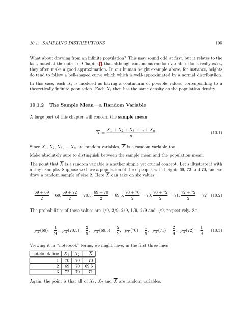
- Page 221 and 222: 10.1. SAMPLING DISTRIBUTIONS 197 Ap
- Page 223 and 224: 10.3. CONFIDENCE INTERVALS FOR MEAN
- Page 225 and 226: 10.4. MEANING OF CONFIDENCE INTERVA
- Page 227 and 228: 10.5. GENERAL FORMATION OF CONFIDEN
- Page 229 and 230: 10.7. CONFIDENCE INTERVALS FOR PROP
- Page 231 and 232: 10.7. CONFIDENCE INTERVALS FOR PROP
- Page 233 and 234: 10.8. CONFIDENCE INTERVALS FOR DIFF
- Page 235 and 236: 10.8. CONFIDENCE INTERVALS FOR DIFF
- Page 237 and 238: 10.8. CONFIDENCE INTERVALS FOR DIFF
- Page 239 and 240: 10.10. R COMPUTATION 215 algebra, w
- Page 241 and 242: 10.13. OTHER CONFIDENCE LEVELS 217
- Page 243 and 244: 10.14. ONE MORE TIME: WHY DO WE USE
- Page 245 and 246: Chapter 11 Introduction to Signific
- Page 247 and 248: 11.2. GENERAL TESTING BASED ON NORM
- Page 249 and 250: 11.5. ONE-SIDED HA 225 By checking
- Page 251 and 252: 11.6. EXACT TESTS 227 It is natural
- Page 253 and 254: 11.8. THE POWER OF A TEST 229 11.8
- Page 255 and 256: 11.9. WHAT’S WRONG WITH SIGNIFICA
- Page 257 and 258: 11.9. WHAT’S WRONG WITH SIGNIFICA
- Page 259 and 260: 11.9. WHAT’S WRONG WITH SIGNIFICA
- Page 261 and 262: Chapter 12 General Statistical Esti
- Page 263 and 264: 12.1. GENERAL METHODS OF PARAMETRIC
- Page 265 and 266: 12.1. GENERAL METHODS OF PARAMETRIC
- Page 267 and 268: 12.1. GENERAL METHODS OF PARAMETRIC
- Page 269 and 270:
12.1. GENERAL METHODS OF PARAMETRIC
- Page 271 and 272:
12.2. BIAS AND VARIANCE 247 people,
- Page 273 and 274:
12.2. BIAS AND VARIANCE 249 Moreove
- Page 275 and 276:
12.3. MORE ON THE ISSUE OF INDEPEND
- Page 277 and 278:
12.4. NONPARAMETRIC DISTRIBUTION ES
- Page 279 and 280:
12.4. NONPARAMETRIC DISTRIBUTION ES
- Page 281 and 282:
12.4. NONPARAMETRIC DISTRIBUTION ES
- Page 283 and 284:
12.5. BAYESIAN METHODS 259 his plan
- Page 285 and 286:
12.5. BAYESIAN METHODS 261 it now b
- Page 287 and 288:
12.5. BAYESIAN METHODS 263 number
- Page 289 and 290:
12.5. BAYESIAN METHODS 265 (b) ˆp,
- Page 291 and 292:
Chapter 13 Simultaneous Inference M
- Page 293 and 294:
13.2. SCHEFFE’S METHOD 269 You ca
- Page 295 and 296:
13.4. OTHER METHODS FOR SIMULTANEOU
- Page 297 and 298:
Chapter 14 Introduction to Model Bu
- Page 299 and 300:
14.1. “DESPERATE FOR DATA” 275
- Page 301 and 302:
14.1. “DESPERATE FOR DATA” 277
- Page 303 and 304:
14.2. ASSESSING “GOODNESS OF FIT
- Page 305 and 306:
14.4. ROBUSTNESS 281 bin width, or
- Page 307 and 308:
14.5. REAL POPULATIONS AND CONCEPTU
- Page 309 and 310:
Chapter 15 Relations Among Variable
- Page 311 and 312:
15.3. ADJUSTING FOR COVARIATES 287
- Page 313 and 314:
15.6. ESTIMATING THAT RELATIONSHIP
- Page 315 and 316:
15.6. ESTIMATING THAT RELATIONSHIP
- Page 317 and 318:
15.7. EXAMPLE: BASEBALL DATA 293
- Page 319 and 320:
15.9. EXAMPLE: BASEBALL DATA (CONT
- Page 321 and 322:
15.11. PREDICTION 297 matter, it ma
- Page 323 and 324:
15.12. PARAMETRIC ESTIMATION OF LIN
- Page 325 and 326:
15.12. PARAMETRIC ESTIMATION OF LIN
- Page 327 and 328:
15.14. DUMMY VARIABLES 303 15.14 Du
- Page 329 and 330:
15.16. WHAT DOES IT ALL MEAN?—EFF
- Page 331 and 332:
15.17. MODEL SELECTION 307 But look
- Page 333 and 334:
15.17. MODEL SELECTION 309 Foundati
- Page 335 and 336:
15.18. WHAT ABOUT THE ASSUMPTIONS?
- Page 337 and 338:
15.19. CASE STUDIES 313 have an und
- Page 339 and 340:
15.19. CASE STUDIES 315 Exercises N
- Page 341 and 342:
15.19. CASE STUDIES 317 8. Consider
- Page 343 and 344:
Chapter 16 Advanced Statistical Est
- Page 345 and 346:
16.2. THE DELTA METHOD: CONFIDENCE
- Page 347 and 348:
16.2. THE DELTA METHOD: CONFIDENCE
- Page 349 and 350:
16.2. THE DELTA METHOD: CONFIDENCE
- Page 351 and 352:
16.2. THE DELTA METHOD: CONFIDENCE
- Page 353 and 354:
16.3. THE BOOTSTRAP METHOD FOR FORM
- Page 355 and 356:
16.3. THE BOOTSTRAP METHOD FOR FORM
- Page 357 and 358:
Chapter 17 Relations Among Variable
- Page 359 and 360:
17.2. THE CLASSIFICATION PROBLEM 33
- Page 361 and 362:
17.2. THE CLASSIFICATION PROBLEM 33
- Page 363 and 364:
17.2. THE CLASSIFICATION PROBLEM 33
- Page 365 and 366:
17.3. NONPARAMETRIC ESTIMATION OF R
- Page 367 and 368:
17.3. NONPARAMETRIC ESTIMATION OF R
- Page 369 and 370:
17.3. NONPARAMETRIC ESTIMATION OF R
- Page 371 and 372:
17.3. NONPARAMETRIC ESTIMATION OF R
- Page 373 and 374:
17.3. NONPARAMETRIC ESTIMATION OF R
- Page 375 and 376:
17.4. SYMMETRIC RELATIONS AMONG SEV
- Page 377 and 378:
17.4. SYMMETRIC RELATIONS AMONG SEV
- Page 379 and 380:
17.4. SYMMETRIC RELATIONS AMONG SEV
- Page 381 and 382:
17.5. SIMPSON’S (NON-)PARADOX 357
- Page 383 and 384:
17.5. SIMPSON’S (NON-)PARADOX 359
- Page 385 and 386:
Chapter 18 Describing “Failure”
- Page 387 and 388:
18.2. A CAUTIONARY TALE: THE BUS PA
- Page 389 and 390:
18.2. A CAUTIONARY TALE: THE BUS PA
- Page 391 and 392:
18.3. RESIDUAL-LIFE DISTRIBUTION 36
- Page 393 and 394:
18.3. RESIDUAL-LIFE DISTRIBUTION 36
- Page 395 and 396:
18.3. RESIDUAL-LIFE DISTRIBUTION 37
- Page 397 and 398:
18.3. RESIDUAL-LIFE DISTRIBUTION 37
- Page 399 and 400:
Chapter 19 Advanced Multivariate Me
- Page 401 and 402:
19.1. CONDITIONAL DISTRIBUTIONS 377
- Page 403 and 404:
19.1. CONDITIONAL DISTRIBUTIONS 379
- Page 405 and 406:
19.1. CONDITIONAL DISTRIBUTIONS 381
- Page 407 and 408:
19.3. MIXTURE MODELS 383 Now that w
- Page 409 and 410:
19.4. TRANSFORM METHODS 385 Thus an
- Page 411 and 412:
19.4. TRANSFORM METHODS 387 19.4.2
- Page 413 and 414:
19.4. TRANSFORM METHODS 389 transfo
- Page 415 and 416:
19.5. VECTOR SPACE INTERPRETATIONS
- Page 417 and 418:
19.7. CONDITIONAL EXPECTATION AS A
- Page 419 and 420:
19.8. PROOF OF THE LAW OF TOTAL EXP
- Page 421 and 422:
19.8. PROOF OF THE LAW OF TOTAL EXP
- Page 423 and 424:
Chapter 20 Markov Chains One of the
- Page 425 and 426:
20.1. DISCRETE-TIME MARKOV CHAINS 4
- Page 427 and 428:
20.1. DISCRETE-TIME MARKOV CHAINS 4
- Page 429 and 430:
20.1. DISCRETE-TIME MARKOV CHAINS 4
- Page 431 and 432:
20.1. DISCRETE-TIME MARKOV CHAINS 4
- Page 433 and 434:
20.1. DISCRETE-TIME MARKOV CHAINS 4
- Page 435 and 436:
20.1. DISCRETE-TIME MARKOV CHAINS 4
- Page 437 and 438:
20.1. DISCRETE-TIME MARKOV CHAINS 4
- Page 439 and 440:
20.2. SIMULATION OF MARKOV CHAINS 4
- Page 441 and 442:
20.4. CONTINUOUS-TIME MARKOV CHAINS
- Page 443 and 444:
20.5. HITTING TIMES ETC. 419 least
- Page 445 and 446:
20.5. HITTING TIMES ETC. 421 First
- Page 447 and 448:
20.5. HITTING TIMES ETC. 423 valued
- Page 449 and 450:
20.5. HITTING TIMES ETC. 425 summon
- Page 451 and 452:
Chapter 21 Introduction to Queuing
- Page 453 and 454:
21.2. M/M/1 429 busy for approximat
- Page 455 and 456:
21.2. M/M/1 431 • Due to the memo
- Page 457 and 458:
21.3. MULTI-SERVER MODELS 433 Recal
- Page 459 and 460:
21.4. LOSS MODELS 435 1 = i,j,k π
- Page 461 and 462:
21.5. NONEXPONENTIAL SERVICE TIMES
- Page 463 and 464:
21.6. REVERSED MARKOV CHAINS 439 So
- Page 465 and 466:
21.6. REVERSED MARKOV CHAINS 441 21
- Page 467 and 468:
21.6. REVERSED MARKOV CHAINS 443 Re
- Page 469 and 470:
21.7. NETWORKS OF QUEUES 445 • Gi
- Page 471 and 472:
21.7. NETWORKS OF QUEUES 447 Let Li
- Page 473 and 474:
Appendix A Review of Matrix Algebra
- Page 475 and 476:
A.2. MATRIX TRANSPOSE 451 • Matri
- Page 477 and 478:
A.6. EIGENVALUES AND EIGENVECTORS 4
- Page 479 and 480:
Appendix B R Quick Start Here we pr
- Page 481 and 482:
B.3. FIRST SAMPLE PROGRAMMING SESSI
- Page 483 and 484:
B.4. SECOND SAMPLE PROGRAMMING SESS
- Page 485 and 486:
B.4. SECOND SAMPLE PROGRAMMING SESS
- Page 487 and 488:
B.6. COMPLEX NUMBERS 463 B.6 Comple