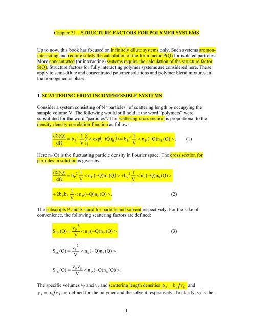
structure factors for polymer systems - NIST Center for Neutron ...

Chapter 31 – STRUCTURE FACTORS FOR POLYMER SYSTEMS
Up to now, this book has focused on infinitely dilute systems only. Such systems are noninteracting
and require solely the calculation of the form factor P(Q) for isolated particles.
More concentrated (or interacting) systems require the calculation of the structure factor
S(Q). Structure factors for fully interacting polymer systems are considered here. These
apply to semi-dilute and concentrated polymer solutions and polymer blend mixtures in
the homogeneous phase.
1. SCATTERING FROM INCOMPRESSIBLE SYSTEMS
Consider a system consisting of N “particles” of scattering length bP occupying the
sample volume V. The following would still hold if the word “polymers” were
substituted for the word “particles”. The scattering cross section is proportional to the
density-density correlation function as follows:
dΣ(
Q)
= b
dΩ
2
P
1
V
N
∑ < exp −
i,
j
r r 2 1
( iQ.
r ) >= b < n ( −Q)
n ( Q)
>
ij
P
1
V
P
P
. (1)
Here nP(Q) is the fluctuating particle density in Fourier space. The cross section for
particles in solution is given by:
dΣ(
Q)
= b
dΩ
2
P
1
V
< n
P
( −Q)
n
P
( Q)
> + b
2
S
1
V
< n ( −Q)
n ( Q)
>
1
+ 2bP bS
< n P ( −Q)
nS
( Q)
> . (2)
V
The subscripts P and S stand for particle and solvent respectively. For the sake of
convenience, the following scattering factors are defined:
2
SPP P
(3)
vP
( Q)
= < n P ( −Q)
n ( Q)
>
V
2
vS
( Q)
= < n S ( −Q)
n ( Q)
>
V
SSS S
v Pv
S
( Q)
= < n P ( −Q)
n ( Q)
> .
V
SPS S
The specific volumes vP and vS and scattering length densities ρ P = b P v P and
ρ = b v are defined for the polymer and the solvent respectively. To clarify, vP is the
S
S
S
S
S

monomer volume and vS is the volume of the solvent molecule. The scattering cross
section becomes:
dΣ(
Q)
= ρ
dΩ
2
P
S
PP
( Q)
+ ρ
2
S
S
SS
( Q)
+ 2ρ
ρ
P
2
S
S
PS
( Q)
. (4)
Most scattering systems are incompressible. It is often convenient to make the following
incompressibility assumption:
v P n P ( Q)
+ vSn
S ( Q)
= 0.
(5)
This introduces the following simplification:
2
2
v S
In other words:
P < n P ( −Q)
n P ( Q)
> = vS
< n S ( −Q)
n ( Q)
>
(6)
= − v < n ( −Q)
n ( Q)
> .
v P S P S
SPP SS
PS
SP
( Q)
= S ( Q)
= −S
( Q)
= −S
( Q)
(7)
This simplifies the cross section to the following form:
dΣ(
Q)
= ( ρ
dΩ
P
− ρ
S
)
2
S
PP
(
Q)
= Δρ
2
S
PP
( Q)
. (8)
This is reasonable since the contrast factor Δρ 2 is always calculated relative to a
“background” scattering length density value. Here, the solvent’s scattering length
density is taken to be that reference value.
2. INTER-PARTICLE INTERACTIONS
Consider a system consisting of N polymers of contrast factor Δρ 2 occupying volume V.
Each polymer comprises n monomers of volume v each so that the polymer volume is vP
= nv. Let us separate out the intra-polymer and the inter-polymer terms in the scattering
cross section as follows:
2
r r
N n r ⎤
( − iQ.
rαiβj
) > + < exp(
− iQ.
rαiβj
) ⎥⎦
dΣ( Q)
⎡ N n
2 v
r
= Δρ
⎢ ∑∑< exp
∑∑ >
dΩ
V ⎣α=
β i,
j
α≠β
i,
j
. (9)
The indices α and β run over the polymer chains and the indices i and j run over the
monomers in a specific polymer chain. Consider a pair of polymer coils (called 1 and 2)
and sum over all pairs.

2
r r
n r ⎤
( − iQ.
r1i
1j
) + N(
N −1)
∑ < exp(
− iQ.
r1i
2 j ) > ⎥⎦
dΣ( Q)
⎡ n
2 v
r
= Δρ
⎢N∑
< exp >
dΩ
V ⎣ i,
j
i,
j
3
. (10)
Note that this formalism holds if the word “particles” were to be substituted for the word
“polymers” assuming (of course) that the particles have internal structure (think
monomers).
Figure 1: Schematic representation of the coordinate system showing a pair of scatterers
that belong to two different polymer coils.
r
The inter-distance between the scattering pair r1i
2 j can be expressed as
r r r r
r = −S
+ S + R and the inter-particle average can be split into the following parts:
1i2
j
1i
exp
2 j
12
r r
r r
r r
r r
( − iQ.
r ) > = < exp(
iQ.
S ) >< exp(
− iQ.
S ) >< exp(
− iQ.
R ) >
< 1i2
j
1i
2 j
12
. (11)
The first two averages are within single particles and the third average is across particles.
The summations become:
n
r r
r r n r r n r r
( − iQ.
S ) =< exp(
− iQ.
R ) > ∑ < exp(
iQ.
S ) > < exp(
− iQ.
S )
∑ < exp >
i,
j
1i2
j
The form factor amplitude is defined as:
F(
Q)
=
R r
coil 1
S1i r
r r 1 n r r
( − iQ.
S ) = < exp(
− iQ.
S )
1 n
∑ < exp 1i
>
n i
1
r
1i
R r
r
2 j
12
R r
12
2
i
r
1i2
j
1i
∑ > .(12)
∑ 2 j > . (13)
n j
j
S2 j
coil 2
r
2 j

The single-particle form factor itself is defined as:
P(
Q)
r r
( − iQ.
S )
1 n
= ∑ < exp 1i1j
> . (14)
2
n i,
j
2
For uniform density particles, the following relation holds P ( Q)
= | F(
Q)
| . This is not
true, however, for non-uniform density object such as polymer coils.
An inter-particle structure factor is defined as:
S
I
( Q)
=
1
N
N
r r
( − iQ.
R )
∑ < exp > . (15)
α,
β
The cross section can therefore be written as follows:
dΣ(
Q)
dΩ
= Δρ
2
2 2
v n N
V
αβ
2
[ P(
Q)
+ | F(
Q)
| ( S ( Q)
−1)
]
4
I
. (16)
r r
Note that the statistical average < exp(
iQ.
r1i
2 j ) > involves integration over the following
r r r
probability distribution P( r1i
, r2
j,
R12
) which can be split to show a conditional probability
r r r r r r r
P( r1i
, r2
j,
R12
) = P(
r1i
, r2
j | R12
) P(
R12
) . For compact scatterers which do not interfere with
r r r
each other’s rotation P( r1i
, r2
j | R12
) is independent of R12 r r
. P( R12
) is the probability of
finding the centers of mass of polymer coils 1 and 2 a distance R12 r
apart.
S
I
( Q)
r r N r r r r
( − iQ.
R ) >= dR
P(
R ) exp(
− iQ.
R )
= N < exp 12 ∫ 12 12
12 . (17)
V
The cross section for systems in this case is given by:
dΣ(
Q)
dΩ
= Δρ
2
2 2
2
v n N ⎡ | F(
Q)
|
P(
Q)
⎢1
+
V ⎣ P(
Q)
( SI
( Q)
−1)
⎥⎦
⎤
. (18)
This result applies to systems with non-spherical symmetry and non-uniform density such
as polymers. Polymer are, however, so highly entangled that an inter-chain structure
factor SI(Q) is meaningless except for dilute solutions whereby polymer coils do not
overlap. Inter-chain interactions for polymer systems are better handled using other
methods described below.
Uniform density scatterers (such as particles) are characterized by
that:
2
P ( Q)
= | F(
Q)
| , so

dΣ(
Q)
dΩ
2
= Δρ
2 2
v n N
P(
Q)
SI
( Q)
. (19)
V
Defining a particles’ volume fraction as φ = Nnv/V, the following result is obtained:
d 2
Σ(
Q)
= Δρ
S(
Q)
dΩ
( Q)
= nφvP(
Q)
S ( Q)
.
S I
This is a well-known result. It is included here even-though it does not apply to polymer
systems so that the derivation does not have to be repeated when covering scattering from
particulate systems later. Note that the scattering factor S(Q) and the inter-particle
structure factor SI(Q) should not be confused; S(Q) has the dimension of a volume
whereas SI(Q) is dimensionless.
3. THE PAIR CORRELATION FUNCTION
Recall the definition for the inter-particle structure factor for a pair of particles (named 1
and 2):
S
I
( Q)
= N < exp
=
1
NV
N
α,
β
r r 1 N r r
( − iQ.
R ) >= < exp(
− iQ.
R )
3
∑ ∫ d R
αβ
∑
N α,
β
εβ >
r r
exp − iQ.
R
r
P(
R ) .
12
( )
r
P( R αβ ) is the probability of finding particle β in volume d 3 Rαβ a distance R αβ
r
away
given that particle α at the origin. When the self term (α = β) is omitted, this result
becomes:
αβ
r r
( iQ.
R )
1 N r
r
3
SI
( Q)
−1
= ∑ ∫ d R εβ exp − αβ P(
R αβ ) (22)
NV α≠β
N r r r r
3
= ∫ d R12
exp(
− iQ.
R12
) P(
R12
) .
V
r
The probability P( R12
) is referred to as the pair correlation function and is often called
r
( R ) . Removing the forward scattering term yields the following well known result:
g 12
S
I
( Q)
−1
=
N
∫ d
V
3
R
12
exp
5
αβ
r r r
3
( − iQ.
R )[ g(
R ) −1]
+ ( 2π)
δ(
Q)
12
12
(20)
(21)
. (23)

The last term (containing the Dirac Delta function) is irrelevant and can be neglected.
r
This last equation shows that SI ( Q)
− 1 and g( R12
) −1
are a Fourier transform pair. Note
r
that g( R12
) peaks at the first nearest-neighbor shell and goes asymptotically to unity at
r r
large distances. The total correlation function is introduced as ( R ) = g(
R ) −1.
4. POLYMER SOLUTIONS
6
h 12
12
In the case of polymer solutions, the Zimm single-contact approximation (Zimm, 1946;
Zimm, 1948) is a simple way of expressing the inter-polymer structure factor. Within that
approximation, the first order term in a “concentration” expansion is as follows:
n
r
2
r vex
⎛ v 2 ⎞
( − iQ.
r ) = − ⎜ n P(
Q)
⎟ + ...
∑ < exp >
i,
j
1 i2
j
V ⎜
⎝ V
vex is a dimensionless factor representing interactions. The cross section becomes an
expansion:
Σ(
Q)
2 ⎡ v ex
= Δρ
⎢S0
( Q)
−
dΩ
⎣ V
d 2
⎟
⎠
( S0
( Q)
) + ... ⎥
⎦
2
(24)
⎤
. (25)
2
This expansion can be resumed as follows 1 x + x ... = 1 ( 1+
x)
dΣ(
Q)
dΩ
= Δρ
2
− to yield:
S0
( Q)
. (26)
v ex
1+
S0
( Q)
V
The bare structure factor for non-interacting polymers has been defined as:
S
0
( Q)
2 2
Nn v
= P(
Q)
= nφvP(
Q)
. (27)
V
Resuming the series extends the single-contact approximation’s applicability range to a
wide concentration regime. The single-contact approximation applies best to semi-dilute
solutions.

Figure 2: Typical interactions that are included and those that are excluded within the
single-contact approximation.
5. THE ZERO CONTRAST METHOD
The zero contrast (or scattering length density match) method also called the high
concentration method for polymer systems consists of using a mixture of deuterated and
non-deuterated polymers and deuterated and non-deuterated solvents in order to isolate
the single-chain form factor; i.e., in order to cancel out the inter-chain interaction terms.
The scattering cross section for a polymer solution containing both deuterated and nondeuterated
polymers is given by:
dΣ(
Q)
dΩ
= Δρ
2
D
S
DD
Included Interactions
( Q)
Excluded Interactions
+
Δρ
2
H
S
HH
( Q)
7
+ 2Δρ
D
Δρ
H
S
HD
( Q)
. (28)
The scattering length density differences between the deuterated (or hydrogenated)
polymer and the solvent are:

Δρ
Δρ
D
H
=
=
⎛ b
⎜
⎝ v
⎛ b
=
⎜
⎝ v
( ) ⎟ D S
ρ − ρ = ⎜ −
D
S
D
b
v
S
⎞
⎠
⎞
.
⎠
( ) ⎟ H S
ρ − ρ −
H
S
H
b
v
S
The various partial scattering factors are split into single-chain parts and inter-chain parts
as follows:
S
I
[ P D ( Q)
+ φ P ( Q)
]
8
(29)
S ( Q)
= n φ v
DD
(30)
DD
D
D
D
S
I
[ P H ( Q)
+ φ P ( Q)
]
S ( Q)
= n φ v
HH
HH
H
H
H
SHD H H H D D D H D HD
I
( Q)
= n φ v n φ v φ φ P ( Q)
.
D
H
Note that the inter-chain structure factors could be negative depending on the volume
fraction. Assume that deuterated and hydrogenated polymers have the same degree of
polymerization ( n D = n H = n P ), and the same specific volume ( v D = v H = v P ), and
define the polymer volume fraction as φ P = φD
+ φH
. The contrast match method consists
in varying the relative deuterated to hydrogenated volume fraction but keeping the total
polymer volume fraction constant.
Define the following “average of the square” and “square of the average” polymer
contrast factors:
2 ⎡ 2 φD
2 φH
⎤
{ Δ P } = ⎢Δρ
D + ΔρH
⎥
⎣ φP
φP
⎦
B (31)
2
2 ⎡ φD
φH
⎤
BP = ⎢Δρ
D + ΔρH
⎥
⎣ φP
φP
⎦
{ }
Δ .
The scattering cross section becomes:
dΣ(
Q)
=
dΩ
2
2
{ ΔB
} n φ v P ( Q)
+ { ΔB
} n φ v P ( Q)
P
P
P
P
S
P
2
2
2
( { Δ } − { ΔB
} ) n φ v P ( Q)
+ { ΔB
} n φ v P ( Q)
= . (32)
BP P P P P S
P P P P T
The following definition has been used:
PT S
P I
( Q)
= P ( Q)
+ φ P ( Q)
. (33)
Note the following simplifications:
P
P
P
I

2
2
2 φDφ
{ BP
} − { ΔBP
} = ( ρD
− ρH
) 2
H
Δ . (34)
φP
φ φ φ φ
Δ .
φ φ φ φ
D
H
D
H
{ BP } = ΔρD
+ ΔρH
= ρD
+ ρH
− ρS
The final result follows:
dΣ(
Q)
=
dΩ
P
P
P
2 D H
D
H
( ρ − ρ ) n φ v P ( Q)
+ ⎜ρ
+ ρ − ρ ⎟ n φ v P ( Q)
D
H
φ
φ
φ
2
P
P
P
P
S
⎛
⎜
⎝
9
D
φ
φ
P
P
H
φ
φ
P
S
⎞
⎟
⎠
2
P
P
P
T
. (35)
Setting the second contrast factor (between the polymer and the solvent) to zero cancels
the second term containing PT(Q) leaving only the first term containing the single-chain
form factor PS(Q). This zero contrast condition is therefore:
φ
φ
D
H
ρ D + ρH
= ρS
. (36)
φP
φP
Note that in general in order to achieve this condition, the solvent must also consist of
mixtures of deuterated and non-deuterated solvents. Defining the following four indices
DP, HP, DS, and HS for deuterated polymer, non-deuterated (hydrogenated) polymer,
deuterated solvent and non-deuterated solvent, the contrast match condition becomes in
the general case:
φ
φ
φ
DP
HP
DS
HS
ρ DP + ρHP
= ρDS
+ ρHS
. (37)
φP
φP
φS
φS
Note that φDP + φHP = φP , φDS + φHS = φP and φP + φS = 1.
6. THE RANDOM PHASE APPROXIMATION
φ
The random phase approximation (de Gennes, 1979, Akcasu-Tombakoglu, 1990;
Hammouda, 1993; Higgins-Benoit, 1994) is a simple mean-field approach used to
calculate the linear response of a homogeneous polymer mixture following a
thermodynamic fluctuation. Consider a binary mixture consisting of a mixture of
polymers 1 and 2 with fluctuating densities n1(Q) and n2(Q). The interaction potentials
between monomers 1 and 2 are W11, W12, W21 and W22. Assume an external perturbation
represented by potentials U1 and U2 and a constraint u that helps apply the
incompressibility assumption. The parameter u can be thought of as a Lagrange
multiplier in an optimization problem with constraints. The constraint here is the
incompressibility condition. The linear response equations follow:

0 ⎡ U1
+ u + W11v1n
1(
Q)
+ W12v
2n
2 ( Q)
⎤
v1
n1
( Q)
= −S11(
Q)
⎢
⎥ (38a)
⎣
k BT
⎦
v
2
n
2
( Q)
= −S
0
22
v1 1
2 2
⎡ U 2 + u + W21v1n
1(
Q)
+ W
( Q)
⎢
⎣
k BT
10
22
v
2
n
2
( Q)
⎤
⎥ (38b)
⎦
n ( Q)
+ v n ( Q)
= 0 . (38c)
The last equation represents the incompressibility constraint. The non-interacting or
“bare” structure factors S ( Q)
0
11 and S ( Q)
0
22 have been defined. These equations have
assumed that no copolymers are present in the homogeneous mixture; i.e., that
0
0
S ( Q)
= S ( Q)
= 0 .
12
21
In order to solve the set of linear equations, we extract the perturbing potential u from the
second equation and substitute it into the first equation to obtain:
0 ⎡U
1 − U 2
⎤
1 n1
( Q)
= −S11(
Q)
⎢ + v11(
Q)
n ( Q)
⎥ . (39)
⎣ k BT
⎦
v 1
This applies along with the following equation representing the response of the fully
interacting system:
⎡U 1 − U 2 ⎤
v1
n1
( Q)
= −S11(
Q)
⎢ ⎥ . (40)
⎣ k BT
⎦
The factor v11(Q) and the Flory-Huggins interaction parameter χ12 are defined as:
v
χ
11
12
( Q)
1
2χ
12
= −
(41)
0
S22
( Q)
v 0
W12
⎛ W11
+ W
= − ⎜
k BT
⎝ 2k
BT
22
Here v0 is a reference volume (often taken to be v 0 = v1v
2 ).
⎟ ⎞
.
⎠
The RPA result for a homogeneous binary blend mixture follows:
1 1 1 2χ
S ( Q)
11
12
= + −
(42)
0
0
S11(Q)
S22
(Q) v 0

0
S11 1 1 1 1
( Q)
= n φ v P ( Q)
.
4
g1
2 2
2 2
[ exp( −Q
R ) −1
Q R ]
2
P 1(
Q)
=
4
g1
+
Q R
Rg1 is the radius of gyration. The incompressibility assumption yields the simplifying
relations:
S11 22
12
( Q)
= S ( Q)
= −S
( Q)
= S(
Q)
. (43)
The scattering cross section is given by:
Σ(
Q)
= ( ρ
dΩ
d 2
1 − ρ2
)
( ρ − ρ )
1
2
dΣ(
Q)
dΩ
2
0
11
S(
Q)
1 1 2χ
= + −
S (Q) S (Q) v
0
22
12
0
This is the so-called de Gennes formula representing the scattering cross section for
polymer blends in the single-phase (mixed phase) region. This is based on the Random
Phase Approximation that applies for long degree of polymerizations (n1>>1 and n2>>2)
and far from the phase boundary condition. This approach does not apply inside the
demixed phase region.
This formalism also applies to polymer solutions by replacing one of the polymers (say
component 2) by solvent; i.e., by setting n2 = 1 and P2(Q) = 1. In the case of polymer
solutions, the excluded volume effect is included in the polymer form factor P1(Q). Note
that the second virial coefficient can be defined for polymer solutions as
= v ( Q = 0)
2 .
A 2 11
The phase separation condition is achieved when the scattering intensity “blows up”; i.e.,
in the limit ( Q = 0)
→ ∞ . This is achieved for
S
0
11
S 11
( 0)
.
11
g1
(44)
0 2χ12
0 0
+ S22
( 0)
− S11(
0)
S22
( 0)
= 0 . (45)
v
0
This is the so-called spinodal condition. Note that with the simplifying assumptions that
n1 = n2 = n, v1 = v2 = v0 and φ1 = φ2 = 0.5, the spinodal condition for polymer blends
simplifies to n 2 = χ .
12

7. THE ISOTHERMAL COMPRESSIBILITY FACTOR
Most mixed polymer systems have finite compressibility. The scattering cross section
consists of a Q-dependent coherent scattering term which is a good monitor of the
structure, a Q-independent incoherent scattering term (mostly from hydrogen scattering),
and another Q-independent “isothermal compressibility” term expressed as:
⎡ dΣ
⎤
⎢
⎣dΩ
⎥
⎦
iso−comp
= Δρ
2
k
B
T χ
T
. (46)
Here Δρ 2 is the contrast factor, kBT is the temperature in energy units and χT is the
isothermal compressibility which is defined as:
1 ⎛ ∂V
⎞
χ T = − ⎜ ⎟ . (47)
V ⎝ ∂P
⎠
T
The isothermal compressibility term is usually small compared to the other terms. For
example, χT = 4.57*10 -4 cm 3 /J for pure water at 25 o C and atmospheric pressure (Weast,
1984). χT is set equal to zero altogether for incompressible mixtures.
REFERENCES
B. Zimm, “Application of the Methods of Molecular Distribution to Solutions of Large
Molecules”, J. Chem. Phys. 14, 164 (1946); and B. Zimm, “The Scattering of Light and
the Radial Distribution Function of High Polymer Solutions”, J. Chem. Phys. 16, 1093
(1948).
P.G. de Gennes, "Scaling Concepts in Polymer Physics", Cornell University Press, New
York (1979).
A.Z. Akcasu and M. Tombakoglu, “Dynamics of Copolymer and Homopolymer Mixtures
in Bulk and in Solution via the Random Phase Approximation”, Macromolecules 23,
607-612 (1990)
B. Hammouda, "SANS from Homogeneous polymer Mixtures: A Unified Overview",
Advances in Polymer Science 106, 87 (1993).
J.S. Higgins and H. Benoit, "Polymers and Neutron Scattering", Oxford (1994).
R.C. Weast, Editor-in-Chief, “CRC Handbook of Chemistry and Physics”, CRC Press
(1984)
12

QUESTIONS
1. What is the primary effect of the incompressibility assumption on the scattering cross
section?
2. If an incompressible polymer solution is characterized by one (independent) structure
factor, how many structure factors describe the equivalent compressible solution?
3. What is the Zimm single-contact approximation?
4. Does the inter-chain structure factor (with excluded volume) for dilute polymer
solutions tend to increase or decrease the scattering intensity at low-Q?
5. What is the use of the zero contrast condition in concentrated polymer systems? What
is the procedure to follow?
6. The Random Phase Approximation applies in what conditions?
7. What is the origin of monomer/monomer interactions in polymer mixtures?
8. Are polymer chains in mixed polymer blends characterized by excluded volume; i.e.,
are they swollen?
9. What is the pair correlation function g(r)?
10. Estimate kBTχT (χT is the isothermal compressibility) for pure water for 25 o C and 1
atmosphere pressure.
ANSWERS
1. The primary effect of the incompressibility assumption is to simplify the scattering
dΣ(
Q)
2
2
cross section from its full form = ρP
SPP
( Q)
+ ρS
SSS
( Q)
+ 2ρ
Pρ
SSPS
( Q)
(where P
dΩ
and S represent the polymer and the solvent respectively) to its simplified form
dΣ(
Q)
2
2
= ( ρP
− ρS
) SPP
( Q)
= Δρ
SPP
( Q)
. This is due to the incompressibility condition
dΩ
relating the various partial structure factors SPP ( Q)
= SSS
( Q)
= −SPS
( Q)
= −SSP
( Q)
.
2. An incompressible polymer solution is characterized by one structure factor SPP(Q).
The equivalent compressible polymer solution is described by three structure factors:
SPP(Q), SSS(Q) and SPS(Q).
3. The Zimm single-contact approximation assumes that inter-chain interactions occur
only through single contacts or chains of single contacts. Double contacts within the same
chain or between two different chains or higher order contacts are not included.
4. The inter-chain structure factor (with excluded volume) for dilute solutions decreases
the scattering intensity at low-Q. Recall the negative sign in Zimm’s single-contact
dΣ( Q)
2 ⎡ v ex
2 ⎤
approximation formula: = Δρ
⎢S0
( Q)
− ( S0
( Q)
) + ...
dΩ
⎥ .
⎣ V
⎦
5. The contrast match method is a way to extract single-chain properties (such as the
radius of gyration) from concentrated polymer systems. This method consists in using a
mixture of deuterated and non-deuterated polymers and deuterated and non-deuterated
solvents in the zero average contrast condition. This involves varying the deuterated to
non-deuterated polymer fraction but keeping the total polymer fraction constant.
13

6. The Random Phase Approximation applies for high molecular weight polymers in the
single-phase (mixed phase) region. It does not apply in the demixed phase region.
7. Monomers interact with each other and with organic solvent molecules due to Van der
Waals interactions mostly. Hydrogen bonding dominates in water-soluble polymers.
8. Polymer coils follow random walk statistics in mixed polymer blends. They are not
swollen like in polymer solutions. Their form factor is the well-known Debye function.
9. The pair correlation function g(r) is the probability of finding a scatterer at a radial
distance r from another scatterer at the origin.
10. kBT = 1.38*10 -23 [J.K -1 ]*295 [K] = 4.112*10 -21 [J] and χT = 4.57*10 -4 cm 3 /J so that
kBT χT = 1.879*10 -24 cm 3 .
14