Left endpoint approximation

2
1.8
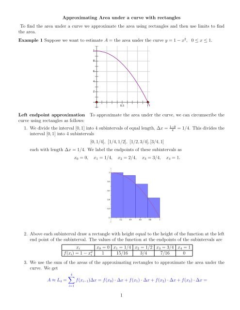
Approximating Area under a curve with rectangles
1.6
To find the area under a curve we approximate the area using rectangles and then use limits to find
1.4
the area.
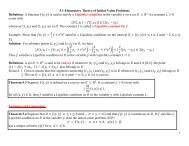
Example 1 Suppose we want to estimate A = the area under the curve y = 1 − x2 1.2
, 0 ≤ x ≤ 1.
f( x)
= 1 – x2 1
0.8
0.6
0.4
0.2
– 1.5 – 1 – 0.5 0.5 1 1.5
– 0.2
Left endpoint approximation To approximate the area under the curve, we can circumscribe the
curve using rectangles as follows:
– 0.4
1. We divide the interval [0, 1] into 4 subintervals of equal length, ∆x =
– 0.6
1−0 = 1/4. This divides the
4
interval [0, 1] into 4 subintervals
[0, 1/4], [1/4, 1/2], [1/2, 3/4], [3/4, 1]
– 0.8
each with length ∆x = 1/4. We label the endpoints of these subintervals as
– 1
x0 = 0, x1 = 1/4, x2 = 2/4, x3 = 3/4, x4 = 1.
– 1.2
– 1.4
– 1.6
– 1.8
– 2
– 2.2
2. Above each subinterval draw a rectangle with height equal to the height of the function at the left
end point of the subinterval. The values of the function at the endpoints of the subintervals are
xi x0 = 0 x1 = 1/4 x2 = 1/2 x3 = 3/4 x4 = 1
f(xi) = 1 − x 2 i 1 15/16 3/4 7/16 0
3. We use the sum of the areas of the approximating rectangles to approximate the area under the
curve. We get
4
A ≈ L4 = f(xi−1)∆x = f(x0) · ∆x + f(x1) · ∆x + f(x2) · ∆x + f(x3) · ∆x =
i=1
1

1 · 1/4 + 15/16 · 1/4 + 3/4 · 1/4 + 7/16 · 1/4 = 25/32 = 0.78125
L4 is called the left endpoint approximation or the approximation using left endpoints (of the subintervals)
and 4 approximating rectangles. We see in this case that L4 = 0.78125 > A (because the function
is decreasing on the interval).
There is no reason why we should use the left end points of the subintervals to define the heights of the
approximating rectangles, it is equally reasonable to use the right end points of the subintervals, or the
midpoints or in fact a random point in each subinterval.
Right endpoint approximation In the picture on the left above, we use the right end point
to define the height of the approximating rectangle above each subinterval, giving the height of the
rectangle above [xi−1, xi] as f(xi). This gives us inscribed rectangles. The sum of their areas gives us
The right endpoint approximation, R4 or the approximation using 4 approximating rectangles and right
endpoints. Use the table above to complete the calculation:
A ≈ R4 =
4
f(xi)∆x = f(x1) · ∆x + f(x2) · ∆x + f(x3) · ∆x + f(x4) · ∆x =
i=1
Is R4 less than A or greater than A.
Midpoint Approximation In the picture in the center above, we use the midpoint of the intervals
to define the height of the approximating rectangle. This gives us The Midpoint Approximation or The
Midpoint Rule:
x m i = midpoint x m 1 = 0.125 = 1/8 x m 2 = 0.375 = 3/8 x m 3 = 0.625 = 5/8 x m 4 = 0.625 = 7/8
f(x m i ) = 1 − (x m i ) 2 63/64 55/64 39/64 15/64
A ≈ M4 =
4
i=1
f(x m i )∆x = f(x m 1 )∆x + f(x m 2 )∆x + f(x m 3 )∆x + f(x m 4 )∆x =
General Riemann Sum We can use any point in the interval x ∗ i ∈ [xi−1, xi] to define the height of
the corresponding approximating rectangle as f(x ∗ i ). In the picture on the right we use random points
2

x ∗ i in each interval to produce a rectangle with height f(x ∗ i ). The sum of the areas of the rectangles
gives us an approximation for A.
A ≈
4
i=1
f(x ∗ i )∆x = f(x ∗ 1)∆x + f(x ∗ 2)∆x + f(x ∗ 3)∆x + f(x ∗ 4)∆x
Increasing The Number of Rectangles and taking Limits
When we increase the number of rectangles used, using a smaller value for ∆x ( = the width of the
rectangles), we get a better approximation to the area. You can see this in the pictures below for A =
the area under the curve y = 1 − x 2 , 0 ≤ x ≤ 1. The pictures show the right end point approximations
to A with ∆x = 1/8, 1/16 and 1/128 respectively:
R8 = .6015625000, R16 = .6347656250, R128 = .6627502441
The pictures below show the left end point approximations to the area, A, with ∆x = 1/8, 1/16 and
1/128 respectively.
L8 = .7265625000, L16 = .6972656250, L128 = .6705627441
We see that the room for error decreases as the number of subintervals increases or as ∆x → 0. Thus
we see that
n
n
f(xi)∆x = lim f(x
n→∞
∗ i )∆x
A = lim
n→∞ Rn = lim
n→∞ Ln = lim
∆x→0
i=1
where x ∗ i is any point in the interval [xi−1, xi]. In fact this is our definition of the area under the curve
on the given interval.
3
i=1

Calculating Limits of Riemann sums
The following formulas are sometimes useful in calculating Riemann sums. I have attached some visual
proofs at the end of the lecture.
n
i =
i=1
n(n + 1)
,
2
n
i 2 2.2 (2n + 1)n(n + 1)
= ,
2
6
i=1
1.8
1.6
n
i 3 2 n(n + 1)
=
2
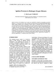
Let us now consider Example 1. We want to find A = the area under the curve y = 1 − x2 1.4
on the
interval [a, b] = [0, 1].
1.2
f( x)
= 1 – x2 1
0.8
0.6
0.4
0.2
– 1.5 – 1 – 0.5 0.5 1 1.5
– 0.2
We know that A = limn→∞ Rn, where Rn is the right endpoint approximation using n approximating
– 0.4
rectangles.
– 0.6
We must calculate Rn and than find limn→∞ – 0.8 Rn.
– 1
1. We divide the interval [0, 1] into n strips of equal length ∆x = 1−0
of the interval [0, 1],
– 1.2
– 1.4
– 1.6
x1 = 0, x2 = 0 + ∆x = 1/n, x3 = 0 + 2∆x = 2/n, . . . , xn−1 = (n − 1)/n, xn = 1.
– 1.8
– 2
2. We will use the right endpoint approximation – 2.2 Rn.
3. The heights of the rectangles can be found from the table below:
4.
i=1
n
= 1/n. This gives us a partition
xi x0 = 0 x1 = 1/n x2 = 2/n x3 = 3/n . . . xn = n/n
f(xi) = 1 − (xi) 2 1 1 − 1/n 2 1 − 2 2 /n 2 1 − 3 2 /n 2 . . . 1 − n 2 /n 2
Rn = f(x1)∆x + f(x2)∆x + f(x3)∆x + · · · + f(xn)∆x =
1 − 1
n2
1
n +
1 − 22
n2
1
n +
1 − 32
n2
1
+ · · · + 1 −
n n2
n2
1
n =
1 1
−
n n2
1
+
n
1 22
−
n n2
1
+
n
1 32
−
n n2
1
+ · · · +
n
1 n2
−
n n2
1
=
n
4

5. Finish the calculation above and find A = limn→∞ Rn using the formula for the sum of squares
and calculating the limit as if Rn were a rational function with variable n.
Riemann Sums in Action: Distance from Velocity/Speed Data
To estimate distance travelled or displacement of an object moving in a straight line over a period of
time, from discrete data on the velocity of the object, we use a Riemann Sum. If we have a table of
values:
time = ti t0 = 0 t1 t2 . . . tn
velocity = v(ti) v(t0) v(t1) v(t2) . . . v(tn)
where ∆t = ti − ti−1, then we can approximate the displacement on the interval [ti−1, ti] by v(ti−1) × ∆t
or v(ti) × ∆t. Therefore the total displacement of the object over the time interval [0, tn] can be
approximated by
or
Displacement ≈ v(t0)∆t + v(t1)∆t + · · · + v(tn−1)∆t Left endpoint approximation
Displacement ≈ v(t1)∆t + v(t2)∆t + · · · + v(tn)∆t Right endpoint approximation
These are obviously Riemann sums related to the function v(t), hinting that there is a connection
between the area under a curve (such as velocity) and its antiderivative (displacement). This is indeed
the case as we will see later.
When we use speed = |velocity| instead of velocity. the above formulas translate to
and
Distance Travelled ≈ |v(t0)|∆t + |v(t1)|∆t + · · · + |v(tn−1)|∆t
Distance Travelled ≈ |v(t1)|∆t + |v(t2)|∆t + · · · + |v(tn)|∆t
Example The following data shows the speed of a particle every 5 seconds over a period of 30 seconds.
Give the left endpoint estimate for the distance travelled by the particle over the 30 second period.
time in s = ti 0 5 10 15 20 25 30
velocity in m/s = v(ti) 50 60 65 62 60 55 50
5

Appendix
Area under a curve, Summary of method using Riemann sums.
To find the area under the curve y = f(x) on the interval [a, b], where f(x) ≥ 0 for all x in [a, b] and
continuous on the interval:
1. Divide the interval into n strips of equal width ∆x = b−a.
This divides the interval [a, b] into n
n
subintervals:
[x0 = a, x1], [x1, x2], [x2, x3], . . . , [xn−1, xn = b].
(Note x1 = a+∆x, x2 = a+2∆x, x3 = a+3∆x, . . . xn−1 = a+(n−1)∆x, xn = a+n∆x = b.)
2. For each interval, pick a sample point, x ∗ i in the interval [xi−1, xi].
3. Construct an approximating rectangle above the subinterval [xi−1, xi] with height f(x ∗ i ). The area
of this rectangle is f(x ∗ i )∆x.
4. The total area of the approximating rectangles is
(The sum is called a Riemann Sum.)
f(x ∗ 1)∆x + f(x ∗ 2)∆x + · · · + f(x ∗ n)∆x
5. We define the area under the curve y = f(x) on the interval [a, b] as
A = lim
n→∞ [f(x ∗ 1)∆x + f(x ∗ 2)∆x + · · · + f(x ∗ n)∆x]
= lim
n→∞ Rn = lim
n→∞ [f(x1)∆x + f(x2)∆x + · · · + f(xn)∆x]
= lim
n→∞ Ln = lim
n→∞ [f(x0)∆x + f(x1)∆x + · · · + f(xn−1)∆x].
(In a more advanced course, you would prove that all of these limits give the same number A which we
use as a measure/definition of the area under the curve)
6

Extra Example Estimate the area under the graph of f(x) = 1/x from x = 1 to x = 4 using six
approximating rectangles and
∆x = b−a
n
= , where [a, b] = [1, 4] and n = 6.
Mark the points x0, x1, x2, . . . , x6 which divide the interval [1, 4] into six subintervals of equal length on
the following axis:
Fill in the following tables:
xi x0 = x1 = x2 = x3 = x4 = x5 = x6 =
f(xi) = 1/xi
(a) Find the corresponding right endpoint approximation to the area under the curve y = 1/x on the
interval [1, 4].
R6 =
(b) Find the corresponding left endpoint approximation to the area under the curve y = 1/x on the
interval [1, 4].
L6 =
(c) Fill in the values of f(x) at the midpoints of the subintervals below:
midpoint = x m i x m 1 = x m 2 = x m 3 = x m 4 = x m 5 = x m 6 =
f(x m i ) = 1/x m i
Find the corresponding midpoint approximation to the area under the curve y = 1/x on the interval
[1, 4].
M6 =
7

Extra Example Estimate the area under the graph of f(x) = 1/x from x = 1 to x = 4 using six
approximating rectangles and
∆x = b−a
n
= 4−1
6
1 = , where [a, b] = [1, 4] and n = 6.
2
Mark the points x0, x1, x2, . . . , x6 which divide the interval [1, 4] into six subintervals of equal length on
the following axis:
Fill in the following tables:
xi x0 = 1 x1 = 3/2 x2 = 2 x3 = 5/2 x4 = 3 x5 = 7/2 x6 = 4
f(xi) = 1/xi 1 2/3 1/2 2/5 1/5 2/7 1/4
(a) Find the corresponding right endpoint approximation to the area under the curve y = 1/x on the
interval [1, 4].
R6 = f(x1)∆x + f(x2)∆x + f(x3)∆x + f(x4)∆x + f(x5)∆x + f(x6)∆x
= 2 1 1 1 2 1 1 1 2 1 1 1
· + · + · + · + · + ·
3 2 2 2 5 2 3 2 7 2 4 2
= 2 1 2 1 2 1
+ + + + + = 1.217857
6 4 10 6 14 8
(b) Find the corresponding left endpoint approximation to the area under the curve y = 1/x on the
interval [1, 4].
L6 = f(x0)∆x + f(x1)∆x + f(x2)∆x + f(x3)∆x + f(x4)∆x + f(x5)∆x
= 1 · 1 2 1 1 1 2 1 1 1 2 1
+ · + · + · + · + ·
2 3 2 2 2 5 2 3 2 7 2
= 1 2 1 2 1 2
+ + + + + = 1.59285
2 6 4 10 6 14
(c) Fill in the values of f(x) at the midpoints of the subintervals below:
midpoint = x m i x m 1 = 5/4 x m 2 = 7/4 x m 3 = 9/4 x m 4 = 11/4 x m 5 = 13/4 x m 6 = 15/4
f(x m i ) = 1/x m i 4/5 4/7 4/9 4/11 4/13 4/15
Find the corresponding midpoint approximation to the area under the curve y = 1/x on the interval
[1, 4].
6
M6 = f(x ∗ i )∆x
i=1
= 4 1 4 1 4 1 4 1 4 1 4 1
· + · + · + · + · + ·
5 2 7 2 9 2 11 2 13 2 15 2
8
= 1.376934

Extra Example Find the area under the curve y = x 3 on the interval [0, 1].
We know that A = limn→∞ Rn, where Rn is the right endpoint approximation using n approximating
rectangles.
We must calculate Rn and than find limn→∞ Rn.
1. We divide the interval [0, 1] into n strips of equal length ∆x = 1−0 = 1/n. This gives us a partition
n
of the interval [0, 1],
x1 = 0, x2 = 0 + ∆x = 1/n, x3 = 0 + 2∆x = 2/n, . . . , xn−1 = (n − 1)/n, xn = 1.
2. We will use the right endpoint approximation Rn.
3. The heights of the rectangles can be found from the table below:
4.
5.
xi x0 = 0 x1 = 1/n x2 = 2/n x3 = 3/n . . . xn = n/n
f(xi) = (xi) 3 0 1/n 3 2 3 /n 3 3 3 /n 3 . . . n 3 /n 3
Rn = f(x1)∆x + f(x2)∆x + f(x3)∆x + · · · + f(xn)∆x =
1
n3
1
n +
3 2
n3
1
n +
3 3
n3
1
3 n
+ · · · +
n n3
1
n =
n i
=
3 1
=
n4 n4 n
i 3 = 1
n4 2 n(n + 1)
2
A = lim
n→∞
1
n4
i=1
i=1
2 n(n + 1) n
= lim
2
n→∞
2 (n + 1) 2
4n4 1 (n + 1)
= lim · ·
n→∞ 4 n
(n + 1)
n
9
= 1
4 .
(n + 1)
= lim
n→∞
2
4n2

Extra Example, estimates from data on rate of change The same principle applies to estimating
Volume from discrete data on its rate of change:
Oil is leaking from a tanker damaged at sea. The damage to the tanker is worsening as evidenced by
the increased leakage each hour, recorded in the following table.
time in h 0 1 2 3 4 5 6 7 8
leakage in gal/h 50 70 97 136 190 265 369 516 720
The following gives the right endpoint estimate of the amount of oil that has escaped from the tanker
after 8 hours:
R8 = 70 · 1 + 97 · 1 + 136 · 1 + 190 · 1 + 265 · 1 + 369 · 1 + 516 · 1 + 720 · 1 = 2363 gallons.
The following gives the right endpoint estimate of the amount of oil that has escaped from the tanker
after 8 hours:
L8 = 50 · 1 + 70 · 1 + 97 · 1 + 136 · 1 + 190 · 1 + 265 · 1 + 369 · 1 + 516 · 1 = 1693 gallons.
Since the flow of oil seems to be increasing over time, we would expect that
L8 < true volume leaked < R8 or the true volume leaked in the first 8 hours is somewhere between 1693
and 2363 gallons.
Visual proof of formula for the sum of integers:
10