Left endpoint approximation

1 · 1/4 + 15/16 · 1/4 + 3/4 · 1/4 + 7/16 · 1/4 = 25/32 = 0.78125
L4 is called the left endpoint approximation or the approximation using left endpoints (of the subintervals)
and 4 approximating rectangles. We see in this case that L4 = 0.78125 > A (because the function
is decreasing on the interval).
There is no reason why we should use the left end points of the subintervals to define the heights of the
approximating rectangles, it is equally reasonable to use the right end points of the subintervals, or the
midpoints or in fact a random point in each subinterval.
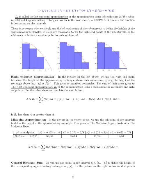
Right endpoint approximation In the picture on the left above, we use the right end point
to define the height of the approximating rectangle above each subinterval, giving the height of the
rectangle above [xi−1, xi] as f(xi). This gives us inscribed rectangles. The sum of their areas gives us
The right endpoint approximation, R4 or the approximation using 4 approximating rectangles and right
endpoints. Use the table above to complete the calculation:
A ≈ R4 =
4
f(xi)∆x = f(x1) · ∆x + f(x2) · ∆x + f(x3) · ∆x + f(x4) · ∆x =
i=1
Is R4 less than A or greater than A.
Midpoint Approximation In the picture in the center above, we use the midpoint of the intervals
to define the height of the approximating rectangle. This gives us The Midpoint Approximation or The
Midpoint Rule:
x m i = midpoint x m 1 = 0.125 = 1/8 x m 2 = 0.375 = 3/8 x m 3 = 0.625 = 5/8 x m 4 = 0.625 = 7/8
f(x m i ) = 1 − (x m i ) 2 63/64 55/64 39/64 15/64
A ≈ M4 =
4
i=1
f(x m i )∆x = f(x m 1 )∆x + f(x m 2 )∆x + f(x m 3 )∆x + f(x m 4 )∆x =
General Riemann Sum We can use any point in the interval x ∗ i ∈ [xi−1, xi] to define the height of
the corresponding approximating rectangle as f(x ∗ i ). In the picture on the right we use random points
2