Left endpoint approximation

More documents

Recommendations

Info

1 · 1/4 + 15/16 · 1/4 + 3/4 · 1/4 + 7/16 · 1/4 = 25/32 = 0.78125 L4 is called the left endpoint approximation or the approximation using left endpoints (of the subintervals) and 4 approximating rectangles. We see in this case that L4 = 0.78125 > A (because the function is decreasing on the interval). There is no reason why we should use the left end points of the subintervals to define the heights of the approximating rectangles, it is equally reasonable to use the right end points of the subintervals, or the midpoints or in fact a random point in each subinterval. Right endpoint approximation In the picture on the left above, we use the right end point to define the height of the approximating rectangle above each subinterval, giving the height of the rectangle above [xi−1, xi] as f(xi). This gives us inscribed rectangles. The sum of their areas gives us The right endpoint approximation, R4 or the approximation using 4 approximating rectangles and right endpoints. Use the table above to complete the calculation: A ≈ R4 = 4 f(xi)∆x = f(x1) · ∆x + f(x2) · ∆x + f(x3) · ∆x + f(x4) · ∆x = i=1 Is R4 less than A or greater than A. Midpoint Approximation In the picture in the center above, we use the midpoint of the intervals to define the height of the approximating rectangle. This gives us The Midpoint Approximation or The Midpoint Rule: x m i = midpoint x m 1 = 0.125 = 1/8 x m 2 = 0.375 = 3/8 x m 3 = 0.625 = 5/8 x m 4 = 0.625 = 7/8 f(x m i ) = 1 − (x m i ) 2 63/64 55/64 39/64 15/64 A ≈ M4 = 4 i=1 f(x m i )∆x = f(x m 1 )∆x + f(x m 2 )∆x + f(x m 3 )∆x + f(x m 4 )∆x = General Riemann Sum We can use any point in the interval x ∗ i ∈ [xi−1, xi] to define the height of the corresponding approximating rectangle as f(x ∗ i ). In the picture on the right we use random points 2
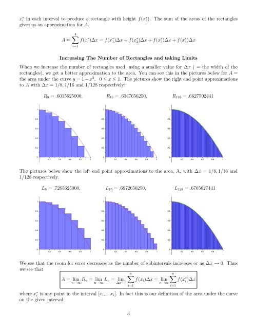
x ∗ i in each interval to produce a rectangle with height f(x ∗ i ). The sum of the areas of the rectangles gives us an approximation for A. A ≈ 4 i=1 f(x ∗ i )∆x = f(x ∗ 1)∆x + f(x ∗ 2)∆x + f(x ∗ 3)∆x + f(x ∗ 4)∆x Increasing The Number of Rectangles and taking Limits When we increase the number of rectangles used, using a smaller value for ∆x ( = the width of the rectangles), we get a better approximation to the area. You can see this in the pictures below for A = the area under the curve y = 1 − x 2 , 0 ≤ x ≤ 1. The pictures show the right end point approximations to A with ∆x = 1/8, 1/16 and 1/128 respectively: R8 = .6015625000, R16 = .6347656250, R128 = .6627502441 The pictures below show the left end point approximations to the area, A, with ∆x = 1/8, 1/16 and 1/128 respectively. L8 = .7265625000, L16 = .6972656250, L128 = .6705627441 We see that the room for error decreases as the number of subintervals increases or as ∆x → 0. Thus we see that n n f(xi)∆x = lim f(x n→∞ ∗ i )∆x A = lim n→∞ Rn = lim n→∞ Ln = lim ∆x→0 i=1 where x ∗ i is any point in the interval [xi−1, xi]. In fact this is our definition of the area under the curve on the given interval. 3 i=1
Page 1: 2 1.8 Approximating Area under a cu
Page 5 and 6: 5. Finish the calculation above and
Page 7 and 8: Extra Example Estimate the area und
Page 9 and 10: Extra Example Find the area under t

Left endpoint approximation

You also want an ePaper? Increase the reach of your titles

Delete template?

Save as template?