A Technique for Drawing Directed Graphs - Graphviz

A Technique for Drawing Directed Graphs
Emden R. Gansner
Eleftherios Koutsofios
Stephen C. North
Kiem-Phong Vo
AT&T Bell Laboratories
Murray Hill, New Jersey 07974
ABSTRACT
We describe a four-pass algorithm for drawing directed graphs. The first pass finds an
optimal rank assignment using a network simplex algorithm. The second pass sets the
vertex order within ranks by an iterative heuristic incorporating a novel weight function and
local transpositions to reduce crossings. The third pass finds optimal coordinates for nodes
by constructing and ranking an auxiliary graph. The fourth pass makes splines to draw
edges. The algorithm makes good drawings and runs fast.
1. Introduction
Drawing abstract graphs is a topic of ongoing research, having such applications as visualization of
programs and data structures, and document preparation. This paper describes a technique for drawing
directed graphs in the plane. The goal is to make high-quality drawings quickly enough for interactive
use. These algorithms are the basis of a practical implementation [GNV1].
1.1 Aesthetic criteria
To make drawings, it helps to assume that a directed graph has an overall flow or direction, such as top
to bottom (assumed in most examples in this paper) or left to right. Such flows can be seen in handmade
drawings of finite automata where the flow is from initial to terminal states, or in data flow graphs
from input to output. This observation has motivated a collection of methods for drawing digraphs
based on the following aesthetic principles:
A1. Expose hierarchical structure in the graph. In particular, aim edges in the same general direction if
possible. This aids finding directed paths and highlights source and sink nodes.
A2. Avoid visual anomalies that do not convey information about the underlying graph. For example,
avoid edge crossings and sharp bends.
A3. Keep edges short. This makes it easier to find related nodes and contributes to A2.
A4. Favor symmetry and balance. This aesthetic has a secondary role in a few places in our algorithm.
There is no way to optimize all these aesthetics simultaneously. For instance, a placement of nodes and
orientation of edges preferred according to A1 may force edge crossings that are undesirable according
to A2. What is more, it is computationally intractable to minimize edge crossings or to find subgraphs

- 2 -
having symmetry. We therefore make some simplifying assumptions and rely on heuristics that run
quickly and make good layouts in common cases. For a survey of other aesthetic principles, we refer
the reader to the annotated bibliography on graph-drawing algorithms by Eades and Tamassia [ET].
1.2 Problem description
The input to the drawing algorithm is an attributed graph G = (V,E) possibly containing loops and
multi-edges. We assume that G is connected, as each connected component can be laid out separately.
The attributes are:
xsize(v) ,ysize(v) Size of bounding box of a node v.
nodesep(G) Minimum horizontal separation between node boxes.
ranksep(G) Minimum vertical separation between node boxes.
ω(e) Weight of an edge e, usually 1. The weight signifies
the edge’s importance, which translates to keeping
the edge short and vertically aligned.
The algorithm assigns each node v to a rectangle in the plane with the center point (x(v) ,y(v) ) and
assigns each edge e to a sequence of B-spline control points (x 0 (e) ,y 0 (e) ) ,... , (x n (e) ,y n (e) ). Though
the unit of these dimensions is not specified, it is convenient to use the traditional coordinate system of
72 units per inch in an implementation. The layout is generally guided by the aesthetic criteria A1-A4,
and specifically by the graph attributes. The details of these constraints will be supplied in the following
sections.
The user can further constrain the layout in a way that is useful for drawing graphs that have time-lines
or for highlighting source and sink nodes. The initial pass of the algorithm described in the next section
assigns nodes to discrete ranks 0...Max_rank. Nodes in the same rank receive the same Y coordinate
value. The user may provide sets S max ,S min ,S 0 ,S 1 , . . . , S k !subset V. These are (possibly empty)
sets of nodes that must be placed together on the maximum, minimum, or same rank, respectively.
1.3 Related work
Drawing digraphs using an iterative method to reduce edge crossing was first studied by Warfield [Wa],
and similar methods were discovered by Carpano [Ca] and Sugiyama, Tagawa, and Toda [STT].
Di Battista and Tamassia describe an algorithm for embedding planar acyclic digraphs such that all edges
flow in the same direction [DT]. We view our work as building on the approach of Warfield, Sugiyama
et al.

1.4 Overview
- 3 -
The graph drawing algorithm has four passes, as shown in figure 1-1. The first pass places the nodes in
discrete ranks. The second sets the order of nodes within ranks to avoid edge crossings. The third sets
the actual layout coordinates of nodes. The final pass finds the spline control points for edges.
1. procedure draw_graph()
2. begin
3. rank();
4. ordering();
5. position();
6. make_splines();
7. end
Figure 1-1. Main algorithm
Our contributions are: (1) an efficient way of ranking the nodes using a network simplex algorithm; (2)
improved heuristics to reduce edge crossings; (3) a method for computing the node coordinates as a rank
assignment problem; and (4) a method for setting spline control points. Techniques (1) and (2) were
first implemented in the graph drawing program dag, described in [GNV1]. Further work, especially (3)
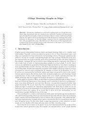
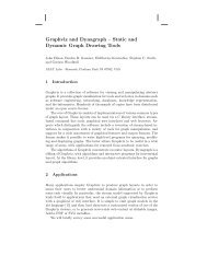
and (4), have been incorporated in dot [KN], a successor to dag. Figures 1-2 and 1-3 are samples of
dot’s output with the corresponding input files.

27
S8
9
42
T24
S24
25
26
4
43
S35
T1
- 4 -
11 3 41 19 14
S1
10 2
38 40 13 17
12
S30
5
39
37
6 T35
7
T8
21 20 16 28
22
23
36
15 29
Figure 1-2a.
(1.11 sec. user time on a Sun-4/280)
digraph world_dynamics {
size="6,6";
S8 -> 9; S24 -> 27; S24 -> 25; S1 -> 10; S1 -> 2; S35 -> 36;
S35 -> 43; S30 -> 31; S30 -> 33; 9 -> 42; 9 -> T1; 25 -> T1;
25 -> 26; 27 -> T24; 2 -> 3; 2 -> 16; 2 -> 17; 2 -> T1; 2 -> 18;
10 -> 11; 10 -> 14; 10 -> T1; 10 -> 13; 10 -> 12;
31 -> T1; 31 -> 32; 33 -> T30; 33 -> 34; 42 -> 4; 26 -> 4;
3 -> 4; 16 -> 15; 17 -> 19; 18 -> 29; 11 -> 4; 14 -> 15;
37 -> 39; 37 -> 41; 37 -> 38; 37 -> 40; 13 -> 19; 12 -> 29;
43 -> 38; 43 -> 40; 36 -> 19; 32 -> 23; 34 -> 29; 39 -> 15;
41 -> 29; 38 -> 4; 40 -> 19; 4 -> 5; 19 -> 21; 19 -> 20;
19 -> 28; 5 -> 6; 5 -> T35; 5 -> 23; 21 -> 22; 20 -> 15; 28 -> 29;
6 -> 7; 15 -> T1; 22 -> 23; 22 -> T35; 29 -> T30; 7 -> T8;
23 -> T24; 23 -> T1;
}
Figure 1-2b. Graph File Listing
18
T30
34
33
31
32

1972
1976
1978
1980
1982
1984
1986
1988
1990
future
v9sh
rc
- 5 -
Bourne
esh vsh
Formshell
Mashey
ksh System-V
ksh-i
KornShell Perl
ksh-POSIX
Figure 1-3a.
Bash
Thompson
(0.50 sec. user time on a Sun-4/280)
digraph shells {
size="7,8";
node [fontsize=24, shape = plaintext];
1972 -> 1976 -> 1978 -> 1980 -> 1982 -> 1984 -> 1986 -> 1988
-> 1990 -> future;
}
node [fontsize=20, shape = box];
{ rank = same; 1976 Mashey Bourne; }
{ rank = same; 1978 Formshell csh; }
{ rank = same; 1980 esh vsh; }
{ rank = same; 1982 ksh "System-V"; }
{ rank = same; 1984 v9sh tcsh; }
{ rank = same; 1986 "ksh-i"; }
{ rank = same; 1988 KornShell Perl rc; }
{ rank = same; 1990 tcl Bash; }
{ rank = same; "future" POSIX "ksh-POSIX"; }
POSIX
Thompson -> {Mashey Bourne csh}; csh -> tcsh;
Bourne -> {ksh esh vsh "System-V" v9sh}; v9sh -> rc;
{Bourne "ksh-i" KornShell} -> Bash;
{esh vsh Formshell csh} -> ksh;
{KornShell "System-V"} -> POSIX;
ksh -> "ksh-i" -> KornShell -> "ksh-POSIX";
Bourne -> Formshell;
/* ’invisible’ edges to adjust node placement */
edge [style=invis];
1984 -> v9sh -> tcsh ; 1988 -> rc -> KornShell;
Formshell -> csh; KornShell -> Perl;
Figure 1-3b. Graph File Listing
csh
tcsh
tcl

2. Optimal Rank Assignment
- 6 -
The first pass assigns each node v member G to an integer rank λ(v) consistent with its edges. This
means that for every e = (v,w) member E, l(e) ≥ δ(e), where the length l(e) of e = (v,w) is defined as
λ(w) − λ(v), and δ(e) represents some given minimum length constraint. δ(e) is usually 1, but can take
any non-negative integer value. δ(e) may be set internally for technical reasons as described below, or
externally if the user wants to adjust the rank assignment. For this pass, each of the nonempty sets
S max ,S min ,S 0 , . . . ,S k is temporarily merged into one node. In addition, loops are ignored, and
multiple edges are merged into one edge whose weight is the sum of the weights of the merged edges.
For efficiency, leaf nodes that are not a member of one of the above sets may be ignored, since the rank
of a leaf is trivially determined in an optimal ranking.
2.1 Making the graph acyclic
A graph must be acyclic to have a consistent rank assignment. Because the input graph may contain
cycles, a preprocessing step detects cycles and breaks them by reversing certain edges [RDM]. Of
course these edges are only reversed internally; arrowheads in the drawing show the original direction.
A useful procedure for breaking cycles is based on depth-first search. Edges are searched in the
‘‘natural order’’ of the graph input, starting from some source or sink nodes if any exist. Depth-first
search partitions edges into two sets: tree edges and non-tree edges [AHU]. The tree defines a partial
order on nodes. Given this partial order, the non-tree edges further partition into three sets: cross edges,
forward edges, and back edges. Cross edges connect unrelated nodes in the partial order. Forward
edges connect a node to some of its descendants. Back edges connect a descendant to some of its
ancestors. It is clear that adding forward and cross edges to the partial order does not create cycles.
Because reversing back edges makes them into forward edges, all cycles are broken by this procedure.
It seems reasonable to try to reverse a smaller or even minimal set of edges. One difficulty is that
finding a minimal set (the ‘‘feedback arc set’’ problem) is NP-complete [EMW] [GJ]. More important,
this would probably not improve the drawings. We implemented a heuristic to reverse edges that
participate in many cycles. The heuristic takes one non-trivial strongly connected component at a time,
in an arbitrary order. Within each component, it counts the number of times each edge forms a cycle in
a depth-first traversal. An edge with a maximal count is reversed. This is repeated until there are no
more non-trivial strongly connected components.
Experiments with this heuristic show that most directed graphs arising from practical applications have a
natural edge direction even when they contain cycles. Graph input usually reflects this natural direction.
In fact, graphs are often created by a graph search performed by some other tool. Reversing an
inappropriate edge disturbs the drawing. For instance, even when a procedure call graph has cycles, one
still expects to see top-level functions near the top of the drawing, and not somewhere in the middle.
From the standpoint of stability, the depth-first, cycle-breaking heuristic seems preferable. It also makes
more informative drawings than would be obtained by collapsing all the nodes in a cycle into one node,
or placing the nodes in a cycle on the same rank, or duplicating one of the nodes in the cycle, as various

esearchers have suggested [Ca] [Ro] [STT].
- 7 -
One other detail is that the nodes representing S max and S min must always have the maximum and
minimum rank assignments. This property is ensured by reversing out-edges of S max and in-edges of
S min. Also, for all nodes v with no in-edge, we make a temporary edge (S min ,v) with δ = 0, and for all
nodes v with no out-edge, we make a temporary edge (v,S max ) with δ = 0. Thus,
λ(S min ) ≤ λ(v) ≤ λ(S max ) for all v.
2.2 Problem Definition
Principle A3 prescribes making short edges. Besides making better layouts, short edges reduce the
running time of later passes whose time depends on the total edge length. So it is desirable to find an
optimal node ranking, i.e., one for which the sum of all the weighted edge lengths is minimal.
Finding an optimal ranking can be reformulated as the following integer program:
min Σ ω(v,w) (λ(w) − λ(v) )
(v,w) member E
subject to: λ(w) − λ(v) ≥ δ(v,w) ∀ (v,w) memberE
The weight function ω and the minimum length function δ as previously described map the edge set E
into the non-negative rational numbers and the non-negative integers, respectively.
There are various ways to solve this integer program in polynomial time. One method is to solve the
equivalent linear program, then transform the solution to an integer one in polynomial time. Another
involves converting the optimal rank assignment problem to an equivalent min-cost flow or circulation
problem, for which there are polynomial-time algorithms (see [GT] and its references). As the constraint
matrix is totally unimodular, the problem can also be solved, though not necessarily in polynomial time,
by applying the simplex method. A more complete discussion of these and other techniques will be
reported in [GNV2].
2.3 Network simplex
Here, we describe a simple approach to the problem based on a network simplex formulation [Ch].
Although its time complexity has not been proven polynomial, in practice it takes few iterations and
runs quickly.
We begin with a few definitions and observations. A feasible ranking is one satisfying the length
constraints l(e) ≥ δ(e) for all e. Given any ranking, not necessarily feasible, the slack of an edge is
the difference of its length and its minimum length. Thus, a ranking is feasible if the slack of every edge
is non-negative. An edge is tight if its slack is zero.
A spanning tree of a graph induces a ranking, or rather, a family of equivalent rankings. (Note that the
spanning tree is on the underlying unrooted undirected graph, and is not necessarily a directed tree.)
This ranking is generated by picking an initial node and assigning it a rank. Then, for each node

- 8 -
adjacent in the spanning tree to a ranked node, assign it the rank of the adjacent node, incremented or
decremented by the minimum length of the connecting edge, depending on whether it is the head or tail
of the connecting edge. This process is continued until all nodes are ranked. A spanning tree is feasible
if it induces a feasible ranking. By construction, all edges in the feasible tree are tight.
Given a feasible spanning tree, we can associate an integer cut value with each tree edge as follows. If
the tree edge is deleted, the tree breaks into two connected components, the tail component containing
the tail node of the edge, and the head component containing the head node. The cut value is defined as
the sum of the weights of all edges from the tail component to the head component, including the tree
edge, minus the sum of the weights of all edges from the head component to the tail component.
Typically (but not always because of degeneracy) a negative cut value indicates that the weighted edge
length sum could be reduced by lengthening the tree edge as much as possible, until one of the head
component-to-tail component edges becomes tight. This corresponds to replacing the tree edge in the
spanning tree with the newly tight edge, obtaining a new feasible spanning tree. It is also simple to see
that an optimal ranking can be used to generate another optimal ranking induced by a feasible spanning
tree. These observations are the key to solving the ranking problem in a graphical rather than algebraic
context. Tree edges with negative cut values are replaced by appropriate non-tree edges, until all tree
edges have non-negative cut values. To guarantee termination, the implementation should employ an
anti-cycling technique, though we have never found this necessary in practice. The resulting spanning
tree corresponds to an optimal ranking. For further discussion of the termination of the network simplex
algorithm and optimality of the result, the interested reader is referred to the literature [Ch] [Cu]
[GNV2].
Figure 2-1 below describes our version of the network simplex algorithm.
1. procedure rank()
2. feasible_tree();
3. while (e = leave_edge()) ≠ nil do
4. f = enter_edge(e);
5. exchange(e,f);
6. end
7. normalize();
8. balance();
9. end
Figure 2-1. Network simplex
Remarks on Figure 2-1.
2: The function feasible_tree constructs an initial feasible spanning tree. This procedure is
described more fully below. The simplex method starts with a feasible solution and maintains this

- 9 -
invariant.
3: leave_edge returns a tree edge with a negative cut value, or nil if there is none, meaning the
solution is optimal. Any edge with a negative cut value may be selected as the edge to remove.
4: enter_edge finds a non-tree edge to replace e. This is done by breaking the edge e, which
divides the tree into a head and tail component. All edges going from the head component to the
tail are considered, with an edge of minimum slack being chosen. This is necessary to maintain
feasibility.
5: The edges are exchanged, updating the tree and its cut values.
7: The solution is normalized by setting the least rank to zero.
8: Nodes having equal in- and out-edge weights and multiple feasible ranks are moved to a feasible
rank with the fewest nodes. The purpose is to reduce crowding and improve the aspect ratio of
the drawing, following principle A4. The adjustment does not change the cost of the rank
assignment. Nodes are adjusted in a greedy fashion, which works sufficiently well. Globally
balancing ranks is considered in a forthcoming paper [GNV2].
1. procedure feasible_tree()
2. init_rank();
3. while tight_tree() < ⎥ V⎥ do
4. e = a non-tree edge incident on the tree
5. with a minimal amount of slack;
6. delta = slack(e);
7. if incident node is e.head then delta = -delta;
8. for v in Tree do v.rank = v.rank + delta;
9. end
10. init_cutvalues();
11. end
Figure 2-2. Finding an initial feasible tree
Remarks on Figure 2-2.
2: An initial feasible ranking is computed. For brevity, init_rank is not given here. Our version
keeps nodes in a queue. Nodes are placed in the queue when they have no unscanned in-edges.
As nodes are taken off the queue, they are assigned the least rank that satisfies their in-edges, and
their out-edges are marked as scanned. In the simplest case, where δ = 1 for all edges, this
corresponds to viewing the graph as a poset and assigning the minimal elements to rank 0. These
nodes are removed from the poset and the new set of minimal elements are assigned rank 1, etc.
3: The function tight_tree finds a maximal tree of tight edges containing some fixed node and
returns the number of nodes in the tree. Note that such a maximal tree is just a spanning tree for
the subgraph induced by all nodes reachable from the fixed node in the underlying undirected

- 10 -
graph using only tight edges. In particular, all such trees have the same number of nodes.
4-8:This finds an edge to a non-tree node that is adjacent to the tree, and adjusts the ranks of the tree
nodes to make this edge tight. As the edge was picked to have minimal slack, the resulting
ranking is still feasible. Thus, on every iteration, the maximal tight tree gains at least one node,
and the algorithm eventually terminates with a feasible spanning tree. This technique is essentially
the one described by Sugiyama et al [STT].
10: The init_cutvalues function computes the cut values of the tree edges. For each tree edge,
this is computed by marking the nodes as belonging to the head or tail component, and then
performing the sum of the signed weights of all edges whose head and tail are in different
components, the sign being negative for those edges going from the head to the tail component.
a
e f
0 0
b
c
g d
-1 3
h
(a)
3
3
3
1
a
e f b
g
h
(b)
2
1 0 2
Figure 2-3. Finding an optimal feasible tree
A small example of running the network simplex algorithm is shown in figure 2-3. Non-tree edges are
dotted, and all edges have weight 1. In (a), the graph is shown after the initial ranking, with cut values
as indicated. For instance, the cut value of edge (g,h) is − 1, corresponding to the weight of edge (g,h)
(from the tail component to the head component) minus the weights of edges (a,e) and (a, f ) (from the
head component to the tail component). In (b), the edge (g,h) with a negative cut value has been
replaced by the non-tree edge (a,e), with the new cut values shown. Because they are all non-negative,
c
d
2
2

the solution is optimal and the algorithm terminates.
2.4 Implementation details
- 11 -
Versions of the network simplex algorithm are well understood and there are results in the literature to
help tune an implementation [Ch]. We feel, however, it is worth pointing out several specific points to
prospective implementors. These optimizations are useful here, but become crucial when we use the
network simplex again in section 4, applied to much larger graphs.
Computing the initial feasible tree and initial cut values is frequently a significant proportion of the cost
in solving the network simplex algorithm. For many graphs in practice, the initial solution is close to
optimal, requiring just a few iterations to reach the final solution. In a naive implementation, initial cut
values can be found by taking every tree edge in turn, breaking it, labeling each node according to
whether it belongs to the head or tail component, and performing the sum. This takes O(VE) time.
To reduce this cost, we note that the cut values can be computed using information local to an edge if
the search is ordered from the leaves of the feasible tree inward. It is trivial to compute the cut value of
a tree edge with one of its endpoints a leaf in the tree, since either the head or the tail component
consists of a single node. Now, assuming the cut values are known for all the edges incident on a given
node except one, the cut value of the remaining edge is the sum of the known cut values plus a term
dependent only on the edges incident to the given node.
We illustrate this computation in figure 2-4 in the case where two tree edges, with known cut values,
join a third, with the shown orientations. The other cases are handled similarly. We assume the cut
values of (u,w) and (v,w) are known. The edges labeled with capital letters represent the set of all
non-tree edges with the given direction and whose heads and tails belong to the components shown.
The cut values of (u,w) and (v,w) are given by
c (u,w) = ω(u,w) + A + C + F − B − E − D
and
c (v,w) = ω(v,w) + L + I + D − K − J − C
respectively. The cut value of (w,x) is then
c (w,x) = ω(w,x) + G − H + A − B + L − K
= ω(w,x) + G − H + (c (u,w) − ω(u,w) − C − F + E + D) + (c (v,w) − ω(v,w) − I − D + J + C)
= ω(w,x) + G − H + c (u,w) − ω(u,w) + c (v,w) − ω(v,w) − F + E − I + J
an expression involving only local edge information and the known cut values. By thus computing cut
values incrementally, we can ensure that every edge is examined only twice. This greatly reduces the
time spent computing initial cut values.

A
C D
B
L
u
F
I
v
- 12 -
Figure 2-4. Incrementally computing cut values.
Another valuable optimization, similar to a technique described in [Ch], is to perform a postorder
traversal of the tree, starting from some fixed root node v root, and labeling each node v with its postorder
traversal number lim(v), the least number low(v) of any descendant in the search, and the edge
parent(v) by which the node was reached (see figure 2-5).
(1,1) (2,2)
v root
(1,3)
K
(4,5)
(4,4)
E
J
(1,9)
w
G
(4,8)
H
(6,6)
x
(7,7)
Figure 2-5. Postorder traversal with nodes labeled by (low,lim).

- 13 -
This provides an inexpensive way to test whether a node lies in the head or tail component of a tree
edge, and thus whether a non-tree edge crosses between the two components. For example, if e = (u,v)
is a tree edge and v root is in the head component of the edge (i.e., lim(u) < lim(v)), then a node w is
in the tail component of e if and only if low(u) ≤ lim(w) ≤ lim(u). These numbers can also be used
to update the tree efficiently during the network simplex iterations. If f = (w,x) is the entering edge, the
only edges whose cut values must be adjusted are those in the path connecting w and x in the tree. This
path is determined by following the parent edges back from w and x until the least common ancestor is
reached, i.e., the first node l such that low(l) ≤ lim(w) ,lim(x) ≤ lim(l). Of course, these postorder
parameters must also be adjusted when exchanging tree edges, but only for nodes below l.
The network simplex is also very sensitive to the choice of the negative edge to replace. We observed
that searching cyclically through all the tree edges, instead of searching from the beginning of the list of
tree edges every time, can save many iterations.
3. Vertex Ordering Within Ranks
After rank assignment, edges between nodes more than one rank apart are replaced by chains of unit
length edges between temporary or ‘‘virtual’’ nodes. The virtual nodes are placed on the intermediate
ranks, converting the original graph into one whose edges connect only nodes on adjacent ranks. Selfedges
are ignored in this pass, and multi-edges are merged as in the previous pass.
The vertex order within ranks determines the edge crossings in the layout, so a good ordering is one
with few crossings. Heuristics are appropriate since minimizing edge crossings in layouts of ranked
graphs is NP-complete, even for only two ranks [EMW].
Several important heuristics for reducing edge crossings in ranked graphs are based on the following
scheme first suggested by Warfield [Wa]. An initial ordering within each rank is computed. Then a
sequence of iterations is performed to try to improve the orderings. Each iteration traverses from the
first rank to the last one, or vice versa. When visiting a rank, each of its vertices is assigned a weight
based on the relative positions of its incident vertices on the preceding rank. Then the vertices in the
rank are re-ordered by sorting on these weights.
Two common vertex weighting methods are the barycenter function [STT] and the median function
[EW]. Let v be a vertex and P the list of positions of its incident vertices on the appropriate adjacent
rank. Note that the position of an adjacent node is only its ordinal number in the current ordering. The
barycenter method defines the weight of v as the average of elements in P. The median method defines
the weight of v as the median of elements in P. When the number of elements in P is even, there are
two medians. This gives rise to two median methods: always using the left median, and always using
the right median. The median method consistently performs better than the barycenter method and has a
slight theoretical advantage since Eades and Wormald [EW] have shown that the median layout of a
two-level graph has no more than 3 times the minimum number of crossings. No such bound is known
for the barycenter method.

- 14 -
Our node ordering heuristic is a refinement of the median method with two major innovations. First,
when there are two median values, we use an interpolated value biased toward the side where vertices
are more closely packed. The second improvement uses an additional heuristic to reduce obvious
crossings after the vertices have been sorted, transforming a given ordering to one that is locally optimal
with respect to transposition of adjacent vertices. It typically provides an additional 20-50% reduction in
edge crossings. We refer the reader to [GNV1] for detailed statistics.
Figure 3-1 shows the node ordering algorithm.
1. procedure ordering()
2. order = init_order();
3. best = order;
4. for i = 0 to Max_iterations do
5. wmedian(order,i);
6. transpose(order);
7. if crossing(order) < crossing(best) then
8. best = order;
9. end
10. return best;
11. end
Figure 3-1. Vertex ordering algorithm
Remarks on Figure 3-1.
2: init_order initially orders the nodes in each rank. This may be done by a depth-first or
breadth-first search starting with vertices of minimum rank. Vertices are assigned positions in
their ranks in left-to-right order as the search progresses. This strategy ensures that the initial
ordering of a tree has no crossings. This is important because such crossings are obvious, easilyavoided
‘‘mistakes.’’
4-9: Max_iterations is the maximum number of iterations. We set Max_iterations to 24.
At each iteration, if the number of crossings improves, the new ordering is saved. In an actual
implementation, one might prefer an adaptive strategy that iterates as long as the solution has
improved at least a few percent over the last several iterations. wmedian re-orders the nodes
within each rank based on the weighted median heuristic. transpose repeatedly exchanges
adjacent vertices on the same rank if this decreases the number of crossings. Both of these
functions are described more completely below.
The weighted median heuristic is shown in figure 3-2. Depending on the parity of the current iteration
number, the ranks are traversed from top to bottom or from bottom to top. To simplify the presentation,
figure 3-2 only shows one direction in detail.

- 15 -
1. procedure wmedian(order,iter)
2. if iter mod 2 == 0 then
3. for r = 1 to Max_rank do
4. for v in order[r] do
5. median[v] = median_value(v,r-1);
6. sort(order[r],median);
7. end
8. else . . .
9. endif
10.
11.
end
12. procedure median_value(v,adj_rank)
13. P = adj_position(v,adj_rank);
14. m = ⎥ P⎥ /2;
15. if ⎥ P⎥ = 0 then
16. return -1.0;
17. elseif ⎥ P⎥ mod 2 == 1 then
18. return P[m];
19. elseif ⎥ P⎥ = 2 then
20. return (P[0] + P[1])/2;
21. else
22. left = P[m-1] - P[0];
23. right = P[⎥ P⎥ -1] - P[m];
24. return (P[m-1]*right + P[m]*left)/(left+right);
25. endif
26. end
Figure 3-2. The weighted median heuristic
Remarks on Figure 3-2.
1-10: In the forward traversal of the ranks, the main loop starts at rank 1 and ends at the maximum
rank. At each rank a vertex is assigned a median based on the adjacent vertices on the previous
rank. Then, the vertices in the rank are sorted by their medians. An important consideration is
what to do with vertices that have no adjacent vertices on the previous rank. In our
implementation such vertices are left fixed in their current positions with non-fixed vertices sorted
into the remaining positions.
12-26: The median value of a vertex is defined as the median position of the adjacent vertices if that
is uniquely defined. Otherwise, it is interpolated between the two median positions using a
measure of tightness. Generally, the weighted median is biased toward the side where vertices are

- 16 -
more closely packed.
13: The adj_position function returns an ordered array of the present positions of the nodes
adjacent to v in the given adjacent rank.
15-16: Nodes with no adjacent vertices are given a median value of -1. This is used within the sort
function to indicate that these nodes should be left in their current positions.
Figure 3-3 shows the transposition heuristic.
1. procedure transpose(rank)
2. improved = True;
3. while improved do
4. improved = False;
5. for r = 0 to Max_rank do
6. for i = 0 to ⎥ rank[r]⎥ -2 do
7. v = rank[r][i];
8. w = rank[r][i+1];
9. if crossing(v,w) > crossing(w,v) then
10. improved = True;
11. exchange(rank[r][i],rank[r][i+1]);
12. endif
13. end
14. end
15. end
16. end
Figure 3-3. The transposition heuristic for reducing edge crossings
Remarks on Figure 3-3.
3-15: This is the main loop that iterates as long as the number of edge crossings can be reduced by
transpositions. As in the loop in the ordering function, an adaptive strategy could be applied
here to terminate the loop once the improvement is a sufficiently small fraction of the number of
crossings.
7-12: Each adjacent pair of vertices is examined. Their order is switched if this reduces the number of
crossings. The function crossing(v,w) simply counts the number of edge crossings if v
appears to the left of w in their rank.
One small point is that the original graph may have edges between nodes on the same rank. We call
these ‘‘flat edges.’’ Following criterion A1, we try to aim them all in the same direction across the
rank. If ranks are ordered from top to bottom, flat edges generally point from left to right. This
involves some minor modifications to the vertex ordering algorithms. If there are flat edges, their

- 17 -
transitive closure is computed before finding the vertex order. The vertex order must always embed this
partial order. In particular, the initial order must be consistent with it, and the transpose and the
sort routines must not exchange nodes against the partial order.
When sorting nodes by medians and transposing adjacent nodes, equality can occur when comparing
median values or number of edge crossings. We have found it helpful, and in keeping with the spirit of
A4, to flip nodes with equal values during the sorting or transposing passes on every other forward and
backward traversal.
One final point is that it is generally worth the extra cost to run the vertex ordering algorithm twice:
once for an initial order determined by starting with vertices of minimal rank and searching out-edges,
and the second time by starting with vertices of maximal rank and searching in-edges. This allows one
to pick the better of two different solutions.
4. Node Coordinates
The third pass sets node coordinates. Previous work has treated this as a postprocessing step of the
barycenter or median methods, making local adjustments to avoid bad layouts. Considering node
placement as a separate, well-defined problem, however, yields better layouts and provides a foundation
for further extensions, such as trying to set the vertex order by methods that are more topological than
geometric.
X and Y coordinates are computed in two separate steps. The first step assigns X coordinates to all
nodes (including virtual nodes), subject to the order within ranks already determined. The second step
assigns Y coordinates, giving the same value to nodes in the same rank. The Y coordinate assignment
maintains the minimum separation ranksep(G) between node boxes. Optionally, the separation between
adjacent ranks can be increased to improve the slope of nearly horizontal edges to make them more
readable. Because the Y coordinate step is straightforward, the remainder of this section deals with X
coordinates.
According to the aesthetic principles already mentioned, short, straight edges are preferable to long,
crooked ones. This property of X coordinates is captured in the following integer optimization problem:
min Σ
e = (v,w)
Ω(e) ω(e) ⎪x w − x v ⎪
subject to: x b − x a ≥ ρ(a,b)
where a is the left neighbor of b on the same rank and ρ(a,b) =
_ xsize(a) _______________ + xsize(b)
+ nodesep(G)
2
Ω(e), an internal value distinct from the input edge weight ω(e), is defined to favor straightening long
edges. Since edges between real nodes in adjacent ranks can always be drawn as straight lines, it is
more important to reduce the horizontal distance between virtual nodes, so chains may be aligned
vertically and thus straightened. The failure to straighten long edges can result in a ‘‘spaghetti effect’’

- 18 -
of edges having many different slopes. Accordingly, edges are divided into three types depending on
their end vertices: (1) both real nodes, (2) one real node and one virtual node, or (3) both virtual nodes.
If e, f, and g are edges of types (1), (2), and (3), respectively, then Ω(e) ≤ Ω( f ) ≤ Ω(g). Our
implementation uses 1, 2, and 8. ρ is a function on pairs of adjacent nodes in the same rank giving the
minimum separation between their center points.
There are standard techniques for transforming this problem into a linear program by the addition of
auxiliary variables and inequalities to remove the absolute values [Ch]. As the resulting constraints are
totally unimodular, solving the linear program with the simplex method produces a solution to the
integer program. This is easy to program, and the layouts it gives are aesthetically pleasing.
Unfortunately, the transformation increases the size of the simplex matrix from VE to 2VE + E 2 entries.
Graphs of a few dozen nodes and edges can be drawn in a few seconds, but larger graphs take much
longer, and even the amount of memory available becomes a limitation. So this is not a completely
satisfactory way to make layouts, particularly on smaller computers.
4.1 Heuristic Approach
This approach replaces the linear program with a heuristic for finding X coordinates. The heuristic finds
a ‘‘good’’ initial placement, then iteratively tries to improve it by sweeping up and down the ranks
similar to the vertex ordering algorithm described in the previous section. The heuristic is sketched
below.
1. procedure xcoordinate()
2. xcoord = init_xcoord();
3. xbest = xcoord;
4. for i = 0 to Max_iterations do
5. medianpos(i,xcoord);
6. minedge(i,xcoord);
7. minnode(i,xcoord);
8. minpath(i,xcoord);
9. packcut(i,xcoord);
10. if xlength(xcoord) < xlength(xbest) then
11. xbest = xcoord;
12. end
13. return xbest;
14. end
Figure 4-1. Assigning x-coordinates to vertices

- 19 -
Remarks on Figure 4-1.
2: An initial set of coordinates is computed as follows. For each rank, the left-most node is assigned
coordinate 0. The coordinate of the next node is then assigned a value sufficient to satisfy the
minimal separation from the previous one, and so on. Thus, on each rank, nodes are initially
packed as far left as possible.
4-12: In each iteration, a collection of heuristics is applied to improve the coordinate assignment. If
this results in an improvement over the previous best assignment, the coordinates are saved. The
function xlength implements the objective function from the above optimization problem. In
our implementation, Max_iterations is 8.
5: The median heuristic is based on the observation that the value ⎥ x − x 0⎥ +⎥ x − x 1⎥ + . . . +⎥ x − x i⎥
is minimized when x is the median of the x i. The heuristic assigns each node both an upward and
downward priority given by the weighted sum of its in- and out-edges, respectively. On
downward iterations, nodes are processed in the downward priority order and placed at the median
position of their downward neighbors subject to the placement of higher priority nodes and space
requirements of nodes not yet placed. When there are two medians, taking their mean improves
symmetry (A4). Upward placement is handled similarly.
6: minedge is similar to medianpos but considers only edges between two real nodes. It places
the edge, oriented vertically, as close as possible to the median of the nodes adjacent to either
endpoint of the edge.
7: minnode performs local optimization one node at a time, using a queue. Initially all nodes are
queued. When a node is removed from the queue, it is placed as close as possible to the median
of all its neighbors (both up and down) subject to the separation function ρ. If the node’s
placement is changed, its neighbors are re-queued if not already in the queue. minnode
terminates when it achieves a local minimum.
8: minpath straightens chains of virtual nodes by sequentially finding sub-chains that may be
assigned the same X coordinate.
9: packcut sweeps the layout from left to right, searching for blocks that can be compacted. For
each node, if all the nodes to the right of it can be shifted to the left by some increment without
violating any positioning constraints, the shift is performed. This is performed by an algorithm
that operates on a list of nodes sorted in order of X coordinates. Though the algorithm is
quadratic in the worst case, it performs well in practice since at every possible cut it only needs to
search the nodes in the neighborhood that is affected by the candidate shift.
These heuristics make good layouts quickly, but they are complicated to program and the results are
sometimes noticeably imperfect. Further fine tuning is difficult because the heuristics begin to interfere
with each other.
4.2 Optimal Node Placement
We noticed that the packcut heuristic does not find all subgraphs that could be compacted to improve
the solution. We considered a more general heuristic to search for subgraphs and shift them. We then

- 20 -
observed that this is very similar to the way the network simplex algorithm moves entire subgraphs to
find an optimal rank assignment (see section 2). This suggested that we apply the network simplex
algorithm find optimal node coordinates, using the X coordinates as ‘‘ranks.’’
The method involves constructing an auxiliary graph as illustrated in figure 4-2. This transformation is
the graphical analogue of the algebraic transformation mentioned above for removing the absolute values
from the optimization problem. The nodes of the auxiliary graph G′ are the nodes of the original graph
G plus, for every edge e in G, there is a new node n e. There are two kinds of edges in G′. One edge
class encodes the cost of the original edges. Every edge e = (u,v) in G is replaced by two edges (n e ,u)
and (n e, v) with δ = 0 and ω = ω(e) Ω(e). The other class of edges separates nodes in the same rank. If
v is the left neighbor of w, then G′ has an edge f = e (v,w) with δ( f ) = ρ(v,w) and ω( f ) = 0. This edge
forces the nodes to be sufficiently separated but does not affect the cost of the layout.
n e
e u
e v
u
e
v
Figure 4-2.
We can now consider the level assignment problem on G′, which can be solved using the network
simplex method. Any solution of the positioning problem on G corresponds to a solution of the level
assignment problem on G′ with the same cost. This is achieved by assigning each n e the value
min(x u ,x v ), using the notation of figure 4-2 and where x u and x v are the X coordinates assigned to u
and v in G. Conversely, any level assignment in G′ induces a valid positioning in G. In addition, in an
optimal level assignment, one of e u or e v must have length 0, and the other has length ⎪x u − x v ⎪. This
means the cost of an original edge (u,v) in G equals the sum of the cost of the two edges e u ,e v in G′
and, globally, the two solutions have the same cost, Thus, optimality of G′ implies optimality for G and
solving G′ gives us a solution for G.
Using the auxiliary graph also permits the specification of ‘‘node ports,’’ or edge endpoints offset in the
X direction from the center of the node. This makes it possible to draw pictures of flat records as shown
e (v,w)
w

z
Graphs can
be fun
- 21 -
mid right
b d y
x
Figure 4-3. Node ports in a graph drawing
in figure 4-3. When computing coordinates for nodes in these diagrams, the edge lengths must include
the displacements of the node ports as well as the distance between the node center points. Let e = (u,v)
be an edge and let Δu and Δv be the specified X displacements of the endpoints from the centers of u
and v, respectively. A Δ < 0 indicates the port is to the left of the vertex’s center. Without loss of
generality, assume Δu≤ Δv and let d e = Δv − Δu. d e is a constant since it depends only on the node
ports and not the assignments of u and v. We can now solve the same optimization problem, but the
cost of edge e is now given by Ω(e) ω(e) ⎪x v − x u + d e ⎪. In the auxiliary graph, we now set δ(e u ) = d e
and δ(e v ) = 0. We can then extend the argument above to show that any positioning for G corresponds
to a level assignment for G′; that any optimal level assignment for G′ induces a valid positioning for G;
and, in both cases, we have
l(e u ) + l(e v ) = ⎪x v − x u + d e ⎪ + d e
for all edges (u,v) in G, where l represents the length function in the level assignment on G′. This
equation implies that the optimal costs of the problems on G and G′ always differ by the constant
Σ d e. Therefore, a minimal assignment for G′ corresponds to a minimal assignment for G.
ememberE
The left part of Figure 4-4 exemplifies how port offsets are translated into the δ value of edges in the
auxiliary graph. The right part shows how a solution relates to the original edge.
c

δ = Δv − Δu
x
δ = 0
Δu
4.3 Implementation details revisited
v
u
Δv
- 22 -
Figure 4-4.
The auxiliary graph is considerably larger than the original one. If the original graph has V nodes, E
edges, and R ranks, the graph with ‘‘virtual’’ nodes added has V + D nodes and E + D edges, where D is
the number of ‘‘virtual nodes.’’ The auxiliary graph then has V + E + 2D nodes and V + 2E + 3D − R
edges. This graph requires disproportionately more time to use the network simplex approach.
Consequently, the optimizations to the network simplex algorithm described at the end of section 2 are
crucial for this pass.
Further improvement is possible by noting that it is easy to construct an initial feasible tree for the
auxiliary graph by taking advantage of its structure. To construct a feasible tree, use all edges connecting
nodes in the same rank. For each pair of adjacent ranks, pick an edge f = (u,v) between the ranks and
add both f u and f v in G′ to the tree. This determines the relative placement of all the nodes in the two
ranks. Finally, for every edge e = (w,x) ≠ f between the two ranks, add either e w or e x to the tree
depending on whether w or x is placed leftmost.
Without these improvements, using network simplex to position the nodes took 5 to 10 times longer.
With these improvements, our implementation runs as fast or faster than the heuristic implementation.
We do not doubt that the heuristic in turn could also be tuned further, but the real advantage is that the
network simplex is much simpler code and produces optimal solutions. Also, improvements that could
be difficult to program into the heuristic can be handled in network simplex. As one example, local
symmetry (A4) may be improved by scanning the graph after network simplex terminates. Tree edges
x
v
.
e
u

- 23 -
whose cut value is exactly 0 identify subgraphs that may be adjusted to equalize the slack on their
incident edges without changing the cost of the solution. This could be used to increase symmetry, such
as centering a node with an even number of descendants.
5. Drawing Edges
In our method, edges are drawn as spline curves. Other graph drawing programs of which we are aware
use line segments, and most make no attempt to avoid situations where line segments overlap unrelated
nodes. Although splines are more difficult to program, they yield better drawings and help to satisfy
aesthetic criterion A2.
In dag, edge splines are made by a collection of heuristics that replace the path of line segments
between virtual nodes with various straight and curved segments, as described in [GNV1]. The
drawback is that the splines sometimes bend sharply to turn inside virtual node boxes or to avoid nearby
nodes. The virtual nodes end up being visible in the final layout. This method does not use the
available space effectively.
It is better to try to find the smoothest curve between two points that avoids the ‘‘obstacles’’ of other
nodes or splines. We can then divide the spline routing algorithm into a top half and a bottom half.
The top half computes a polygonal region of the layout where the spline may be drawn. It calls the
bottom half to compute the best spline within the region. As a final step, the top half resizes virtual
nodes according to the bounding box of the spline, and splines and clips the spline to the boundaries of
the endpoint node shapes.
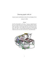
A region and its spline are illustrated in figure 5-1.† The associated edge is from ‘‘Interdata’’ to
‘‘Unix/TS 3.0’’.
More formally, we draw splines by creating and solving instances of the following sub-problem. Given
B 0 , . . . , B m ,q,θ q ,r,θ r where B i are boxes parallel to the coordinate axes, such that B i has edges in
common with B i − 1 and B i + 1; q and r are points on or inside the first and last box respectively, find
s 0 , . . . , s n and BB 0 , . . . , BB m, where s i are the control points of a piecewise Bezier curve and BB i
are boxes parallel to the coordinate axes. The curve must have q and r as its endpoints. θ q and θ r are
optional; if they are specified, then the curve must have the given slope at the corresponding endpoint.
The BB i correspond to the B i and are the smallest boxes that contain the generated splines.
We next describe the two parts of the algorithm.
__________________
† Graph data courtesy of Ian F. Darwin, SoftQuad Inc., and Geoffrey Collyer, Software Tool & Die.

5.1 Finding the Region
- 24 -
There are three kinds of edges in the drawing: edges between nodes on different ranks, flat edges
between different nodes on the same rank, and self-edges or loops.
8th Edition
9th Edition
5th Edition
6th Edition PWB 1.0
1 BSD Interdata LSX Mini Unix Wollongong PWB 1.2 USG 1.0
4.1 BSD
4.2 BSD
4 BSD
4.3 BSD Ultrix-32
5.1.1 Edges between ranks
3 BSD
32V
2 BSD
2.8 BSD
2.9 BSD
7th Edition
Xenix UniPlus+
Ultrix-11
V7M
Unix/TS 1.0
Figure 5-1. Region for a spline
(0.48 sec. user time Sun4-280)
PWB 2.0
Unix/TS 3.0
USG 2.0
USG 3.0
TS 4.0
CB Unix 1
CB Unix 2
CB Unix 3
Unix/TS++ PDP-11 Sys V
In practice, most edges connect nodes on different ranks. The region for this kind of edge has a few
boxes near its tail port, then an alternating sequence of inter-rank boxes and virtual node boxes, and
finally a few boxes near the head port. The tail and head port boxes route the spline to the appropriate
side of the node.
To curve as smoothly as possible, a spline should be allowed all the space that is available. So the
region should include not only virtual node boxes, but also any extra space next to them. After the
spline has been computed, the virtual node boxes are updated according to the BB i, so splines computed
afterward will be able to use all the space remaining but not come too close to splines already drawn.
Because splines are drawn by a ‘‘greedy’’ strategy, they depend on the order in which they are
computed. It seems reasonable to route the shorter splines first because they can often be drawn as
straight lines, but the order does not seem to affect the drawing quality much.
System V.0
System V.2
System V.3

- 25 -
There are three details that can help to improve the appearance of the splines. First, when edges cross,
they should not constrain each other too much. Otherwise, a spline may have an awkward, sharp turn.
This is easily avoided by making an adjustment to the boxes. When setting the size of a box, we ignore
virtual nodes to the left or right that correspond to edges that cross within two ranks. Crossings further
away are not considered because unintended multiple crossings can occur when the boxes become too
sloppy.
Second, when an edge has a section that is almost vertical, it looks better to just draw it as a vertical
line. This is most obvious when edges run alongside each other, because parallel line segments look
better than long segments with slightly different slopes. When the region finding procedure detects a
long vertical section, it terminates the current region, draws its spline, draws the vertical line segment,
and finally begins the region of the rest of the edge. This is one of the situations where θ q and θ r are
used, since the splines must have a vertical tangent at the endpoint where they join the vertical line
segment.
Third, when several splines approach a common termination point, it is important to avoid ‘‘accidental’’
intersections. To do this, we check if there are previously computed splines with the same endpoint. If
so, we find the closest ones to the right and the left. We then subdivide the inter-rank space, and
evaluate the left and right splines at the intervals. These points (or the boundaries of the layout, if one
of the left or right splines does not exist) determine a set of boxes that separate the new spline from the
existing ones as they approach the terminal node. The left and right splines and the boxes that result
can be seen in figure 5-1.
This subdivision of the inter-rank box could be viewed as approximating a polygonal region not
necessarily aligned with the coordinate axes. In some layouts there are other places where non-aligned
boxes or other polygons could prevent unintended tangencies. If we were writing this program again,
we would try general polygons instead of boxes.
Thus far we have not mentioned multiple edges between the same pair of nodes. When these exist, a
spline is computed for one of the edges, and the rest of the edges are drawn by adding an increasing X
coordinate displacement to each one (multiples of nodesep(G) work well). Space for multiple edges
must be reserved in the previous pass, described in section 4, when setting the separation between nodes.
5.1.2 Flat Edges
Flat edges are handled much like inter-rank edges, but the region routes past intervening nodes and
spaces between nodes. We omit most of the details since they are quite similar. One difference is that
if an edge connects two adjacent nodes it is drawn as a single spline with the following control points:

dx = (x(u) − x(v) )
p0 = (x(v) ,y(v) )
1_ p1 = p0 + ( _ dx, 0 )
3
2_ p2 = p0 + ( _ dx, 0 )
3
p3 = (x(u) ,y(u) )
- 26 -
For multiple flat edges, a spline is computed for the first one, and succeeding edges are drawn by adding
Y coordinate displacements. If an edge has a label, the label is positioned halfway along the edge.
5.1.3 Self-edges
Self-edges are drawn as loops on the sides of nodes. If an edge specifies tail or head ports, a polygonal
region is generated that connects the two ports. The orientation of the region may be either clockwise or
counter-clockwise, depending on the positions of the ports. If an edge does not specify tail and head
ports it is drawn as a sequence of two splines, p0 ,... ,p3 and p3 ,... ,p6. These control points are
computed as follows:
dx = nodesep(G)
1_ dy = _ ysize(v)
2
p0 = (x(v) ,y(v) )
1_ p1 = p0 + ( _ dx,dy)
3
2_ p2 = p0 + ( _ dx,dy)
3
p3 = p0 + (dx, 0 )
2_ p4 = p0 + ( _ dx, − dy)
3
1_ p5 = p0 + ( _ dx, − dy)
3
p6 = p0
If there are multiple edges, their loops are nested. If an edge has a label, the label is positioned halfway
along the edge. In the simple case mentioned above, the label is positioned to the right of point p3. In
the case of multiple edges with labels, the sizes of the labels are added to the displacement between
edges. This prevents the curve of one edge crossing over the label of another edge. Space for self edges
is allocated in the previous pass, described in section 4, when setting the separation between adjacent
nodes.
5.2 Computing Splines
The computation of the splines has three stages. First, a piecewise linear curve or path lying entirely
inside the region is computed. Then, the endpoints of this path are used as hints in the computation of a
piecewise Bezier spline. Finally, the actual space used by the curve is computed in terms of the original

- 27 -
boxes. The data structures computed by these three stages are shown in figure 5-4. The region shown
in this figure is the same one as in figure 5-1. This example contains 13 boxes.
The three stages are outlined in figure 5-2.
1. procedure compute_splines (B_array, q, theta_q, use_theta_q, s, theta_s, use_theta_s)
2. compute_L_array (B_array);
3. compute_p_array (B_array, L_array, q, s);
4. if use_theta_q then vector_q = anglevector(theta_q)
5. else vector_q = zero_vector;
6. if use_theta_s then vector_s = anglevector(theta_s)
7. else vector_s = zero_vector;
8. compute_s_array (B_array, L_array, p_array, vector_q, vector_s);
9. compute_bboxes ();
10. end
Figure 5-2. Computing splines
Remarks on Figure 5-2.
2: compute_L_array computes the array L 0 , . . . , L m + 1 where L i is the line segment that is
the intersection of box B i − 1 with box B i. In figure 5-4, these line segments are shown as
3:
thicker lines between boxes. There are 14 such segments.
compute_p_array computes an array of points p 0 , . . . , p k
connects q and s. In figure 5-4, there are 3 such points.
defining a feasible path that
4-7: If use_theta_q or use_theta_s are true, the curve is constrained to approach the
corresponding endpoint at the specified angles. vector_q and vector_s are normalized
vectors.
8: compute_s_array computes an array of points s 0 , . . . , s k defining a piecewise Bezier
spline that connects q and s and lies entirely inside the region. In the worst case, we can have
one Bezier spline per box. In most cases, however, our approach generates significantly fewer
splines. For example, in figure 5-4, there are only 2 splines, one between p 0 and p 1 and one
between p 1 and p 2. In more complex paths, there may even be fewer splines than line
9:
segments, since, unlike a line, a spline can curve around obstacles.
compute_bboxes computes the space actually taken up by the curve. It computes the array
BB 0 , . . . , BB m, where BB i is the narrowest sub-box of B i containing the curve.
compute_p_array and compute_s_array are both implemented as divide-and-conquer methods,
as shown in figure 5-3.

- 28 -
1. procedure compute_p_array (B_array, L_array, q, s)
2. if line_fits (B_array, L_array, q, s) then return;
3. p = compute_linesplit (B_array, L_array);
4. addto_p_array (p);
5. compute_p_array (B_array1, L_array1, q, p);
6. compute_p_array (B_array2, L_array2, p, s);
7.
8.
end
9. procedure compute_s_array (B_array, L_array, p_array, vector_q, vector_s)
10. spline = generate_spline (p_array, vector_q, vector_s);
11. if size (p_array) == 2 then
12. while spline_fits (spline, B_array, L_array) == False do
13. straighten_spline (spline);
14. elseif spline_fits (spline, B_array, L_array) == False then
15. count = 0;
16. ospline = spline;
17. repeat
18. spline = refine_spline (p_array, ospline,
19. mode (count, max_iterations));
20. fits = spline_fits (spline, B_array, L_array);
21. count = count + 1;
22. while (fits == False) and (count

- 29 -
3:
segments.
If the (q, s) line does not fit, compute_linesplit finds the L segment that is the furthest
from the (q, s) line and subdivides B_array and L_array along that segment. p is the one of the
two endpoints of the subdivision segment that is closer to the (q, s) line. In figure 5-4, for
example, the path is subdivided along L 7.
4: addto_p_array adds p to the array of endpoints for the path.
5-6: The two recursive calls to compute_p_array complete the computation of the path.
compute_p_array is not guaranteed to be the shortest path, but it works very well so we
have not developed it further. If it were important, the shortest path could be found in linear
time using convex hulls [Su].
10: generate_spline computes a Bezier spline that approximates the path. This is done using
a common technique [Gl].
11-13: The case where there is only one segment in the path is handled first. spline_fits
checks if the spline lies entirely inside the region. The spline is sampled along its length and
these samples are then clipped as a linear path against the box region. The process is similar to
that of line_fits. As long as the spline does not fit, straighten_spline adjusts the
control points of the spline to reduce the curvature. In the worst case, the spline becomes a
line, and that is known to fit inside the path. This worst case can produce sharp turns. Most of
the time, however, the spline fits inside the region after just a few iterations and this process
does not produce any visual anomalies. It is only when the region itself makes sharp turns that
the worst case may happen.
14-30: The second case is that the path has more than one segment. If the spline does not fit,
refine_spline perturbs the control points of the spline in an attempt to make the spline fit.
The approach is similar to the straightening approach in lines 14-16. We try to decrease the
curvature of the spline. If this does not seem to improve the fit, we try to increase the
curvature. Since this process may never terminate, max_iterations controls how many
times to try. mode returns a flag to indicate if the curvature is to be increased or decreased.
If the spline still does not fit even after the refinement, we subdivide the problem.
compute_splinesplit finds the endpoint of a segment on the path that is the furthest from
the spline and subdivides the box and path arrays along that point. The two recursive calls to
compute_s_array compute two piecewise Bezier splines, each fitting inside its
corresponding part of the region. To force the two curves to join smoothly at the subdivision
point, we also force the two splines to have the same unit tangent vector at that point. This
guaranties C 1 continuity at the subdivision point. Forcing C 2 continuity does not seem to
produce better results and is also much more expensive to compute. The straightening and
refining heuristics, which save a lot of time, are based on the assumption that the tangent
vectors at the endpoints of a spline can be scaled independently of the tangent vectors of the
two adjacent splines. To maintain C 2 continuity, whenever a tangent vector is scaled, the
tangent vector of the adjacent spline must also be scaled so that the two vectors will continue to

- 30 -
have the same length. The scaling can propagate all the way to the end of the region. In
addition, some of these splines may not fit even after scaling, and this would require more
subdivisions, including subdivisions inside a single box. This is more trouble than it is worth.
32: Finally, addto_s_array adds the spline to the piecewise Bezier spline.
5.3 Edge Labels
q = p0 = L0
B5
L2
B6
BB5
Figure 5-4. The three stages
p1
B7
L7
q = p2 = L13
In dag, edge labels are placed next to the midpoint of the spline. This is an oversimplification since the
placement does not avoid or even detect overlapping with other splines, labels, or nodes. Yet, graphs
with edge labels are often small and sparse, so this technique is sometimes adequate.
In dot, edge labels on inter-rank edges are represented as off-center virtual nodes. This guarantees that
labels never overlap other nodes, edges or labels. Certain adjustments are needed to make sure that
adding labels does not affect the length of edges. Setting the minimum edge length to 2 (effectively
doubling the ranks when virtual nodes are created) and halving the separation between ranks
compensates for the label nodes. This makes it at least twice as expensive to draw a graph with labels,
but the labels are readable. Figure 5-5 shows a drawing of a graph with edge labels.
Edge labels on self edges are easy to handle, but flat edges are more complicated. Here we must choose
the left-to-right order for the virtual node of the label so that its X coordinate lies between the endpoint

- 31 -
coordinates, not to the right or the left. At present we are still working on this problem.
More sophisticated placement of labels in diagrams (such as geographic maps) is a difficult research
problem deserving further study. However, it is worth remarking that the label placing program as
described by Freeman and Ahn [FA] is larger than our whole graph drawing program.
LR_0
SS(S)
SS(B)
6. Conclusions
LR_1
LR_2
S($end)
S(A)
SS(b)
LR_3
LR_4
S(b)
LR_6
SS(a)
S(a)
S(a)
LR_5
S(b)
S(a)
S(b)
Figure 5-5. A finite state machine with labeled transitions
(0.15 sec. user time on a Sun-4/280)
We have described a method for drawing digraphs. Our contributions are the application of network
simplex for assigning ranks and final node coordinates, an improved heuristic for reducing edge
crossing, and a method for making edge splines. The method of finding node coordinates allows edges
with X coordinate endpoint displacements. These techniques are straightforward to program, run fast
enough for interactive use, and make drawings that compare well with previous work as to being
readable and visually pleasing.
Further work might address the following:
• Understand how to modify the graph or its layout to enhance readability.
LR_7
S(a)
S(b)
LR_8

- 32 -
• Improve the edge crossing and spline drawing heuristics.
• Allow more interaction between the layout passes. Different solutions having the same cost in one
phase may affect results a great deal in a following phase. For instance, two layouts can have the same
number of crossings but much different final coordinates.
• Support incremental (on-line) graph drawing for animation. Stability from one drawing to the next is
essential.
7. Acknowledgments
The referees made detailed comments that helped us to clarify the presentation, particularly in section 2.
We also wish to thank Guy Jacobson and Steve Lally for their criticisms on content and style.

- 33 -
REFERENCES
[AHU] Aho, A., J. Hopcroft, and J. Ullman, The Design and Analysis of Computer Algorithms,
Addison-Wesley, Reading, Massachusetts, 1974.
[Ca] Carpano, M., ‘‘Automatic display of hierarchized graphs for computer aided decision analysis,’’
IEEE Transactions on Software Engineering SE-12(4), 1980, pp. 538-546.
[Ch] Chvatal, V., Linear Programming, W. H. Freeman, New York, 1983.
[Cu] Cunningham, W. H., ‘‘A network simplex method,’’ Mathematical Programming 11, 1976, pp.
105-116.
[DT] Di Battista, G., and R. Tamassia, ‘‘Algorithms for Plane Representations of Acyclic Digraphs,’’
Theoretical Computer Science 61, 1988, pp. 175--198.
[EMW] Eades, P., B. McKay and N. Wormald, ‘‘On an Edge Crossing Problem,’’ Proc. 9th Australian
Computer Science Conf., 1986, pp. 327-334.
[ET] Eades, P. and Roberto Tamassia, ‘‘Algorithms for Automatic Graph Drawing: An Annotated
Bibliography,’’ Technical Report CS-89-09 (Revised Version), Brown University, Department of
Computer Science, Providence RI, October 1989.
[EW] Eades, P. and N. Wormald, ‘‘The Median Heuristic for Drawing 2-Layers Networks,’’ Technical
Report 69, Dept. of Computer Science, Univ. of Queensland, 1986.
[FA] Freeman, Herbert and John Ahn, ‘‘On The Problem of Placing Names in a Geographic Map,’’
International Journal of Pattern Recognition and Artificial Intelligence, 1(1), 1987, pp. 121-140.
[GJ] Garey, Michael R. and David S. Johnson, Computers and Intractability, W. H. Freeman, San
Francisco, 1979.
[Gl] Glassner, Andrew S., Graphics Gems (editor), Academic Press, San Diego, 1990.
[GNV1] Gansner, E. R., S. C. North and K.-P. Vo, ‘‘DAG - A Program that Draws Directed Graphs,’’
Software - Practice and Experience 17(1), 1988, pp. 1047-1062.
[GNV2] Gansner, E. R., S. C. North and K.-P. Vo, ‘‘On the Rank Assignment Problem,’’ to be
submitted.
[GT] Goldberg, A. V. and R. E. Tarjan, ‘‘Finding minimum-cost circulations by successive
approximation,’’ Mathematics of Operations Research, 15(3), 1990, pp. 430-466.
[Ka] Karmarkar, N., ‘‘A new polynomial-time algorithm for linear programming,’’ Proc. 16th ACM
STOC, Washington, 1984, pp. 302-311.
[Kh] Khachiyan, L. G., ‘‘A polynomial algorithm in linear programming,’’ Sov. Math. Doklady 20,
1979, pp 191-194.
[KN] Koutsofios, E., and S. North, ‘‘Drawing graphs with dot,’’ technical report (available from the
authors), AT&T Bell Laboratories, Murray Hill NJ, 1992.
[Ro] Robbins, G., ‘‘The ISI grapher, a portable tool for diplaying graphs pictorially,’’ Symboliikka
’87, Helsinki, Finland, also Technical Report IST/RS-87-196, Information Sciences Institute,
Marina Del Rey, CA.
[RDM] Rowe, L. A., M. Davis, E. Messinger, C. Meyer, C. Spirakis, and A. Tuan, ‘‘A Browser for
Directed Graphs,’’ Software - Practice and Experience 17(1), January, 1987, pp. 61-76.
[STT] Sugiyama, K., S. Tagawa and M. Toda, ‘‘Methods for Visual Understanding of Hierarchical
System Structures,’’ IEEE Transactions on Systems, Man, and Cybernetics SMC-11(2), February,
1981, pp. 109-125.
[Su] Suri, Subhash. ‘‘A linear time algorithm for minimum link paths inside a simple polygon,’’
Computer Vision, Graphics, and Image Processing 35, 1986, pp. 99-110.
[Ta] Tarjan, R. E. ‘‘Depth first search and linear graph algorithms,’’ SIAM Journal of Computing
1(2), 1972, pp. 146-160.
[Wa] Warfield, John, ‘‘Crossing Theory and Hierarchy Mapping,’’ IEEE Transactions on Systems,
Man, and Cybernetics SMC-7(7), July, 1977, pp. 505-523.