
Create successful ePaper yourself
Turn your PDF publications into a flip-book with our unique Google optimized e-Paper software.
<strong>Drawing</strong> <strong>graphs</strong> <strong>with</strong> <strong>dot</strong><br />
Emden Gansner and Eleftherios Koutsofios and Stephen North<br />
January 26, 2006<br />
Abstract<br />
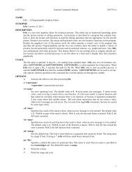
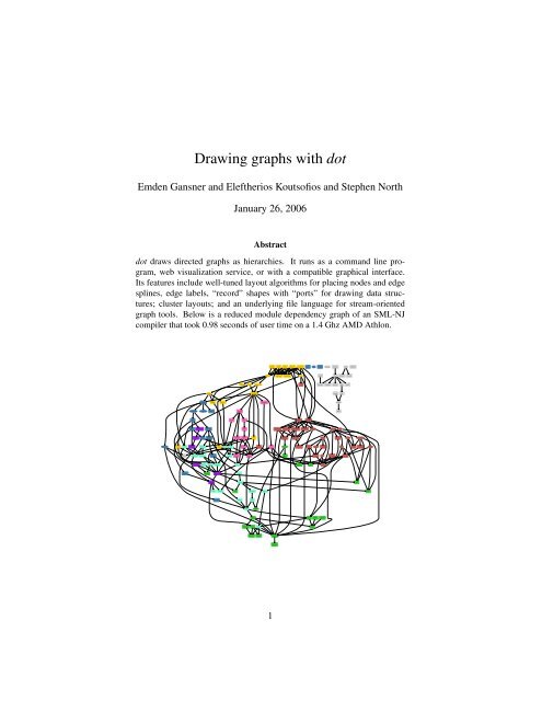
<strong>dot</strong> draws directed <strong>graphs</strong> as hierarchies. It runs as a command line program,<br />
web visualization service, or <strong>with</strong> a compatible graphical interface.<br />
Its features include well-tuned layout algorithms for placing nodes and edge<br />
splines, edge labels, “record” shapes <strong>with</strong> “ports” for drawing data structures;<br />
cluster layouts; and an underlying file language for stream-oriented<br />
graph tools. Below is a reduced module dependency graph of an SML-NJ<br />
compiler that took 0.98 seconds of user time on a 1.4 Ghz AMD Athlon.<br />
MLLexFun<br />
Strs<br />
Index PrintDec Instantiate<br />
Vector<br />
Normalize<br />
NewParse<br />
MLLrValsFun JoinWithArg LrParser<br />
Signs ApplyFunctor CoreLang<br />
SigMatch Misc Typecheck<br />
PrintAbsyn<br />
BareAbsyn PrintBasics<br />
Overload<br />
AbstractFct PrintVal EqTypes PrintType<br />
ArrayExt<br />
Importer<br />
Linkage<br />
Modules<br />
Interp Absyn Equal<br />
ModuleUtil<br />
Fixity Variables<br />
TyvarSet<br />
CoreInfo Unboxed<br />
Lambda<br />
Ascii<br />
Prim<br />
Unify<br />
UnixPaths Interact ModuleComp<br />
TypesUtil<br />
ConRep<br />
Types<br />
ProcessFile<br />
FreeLvar LambdaOpt<br />
Translate<br />
Nonrec MC<br />
MCopt<br />
InlineOps MCprint<br />
Reorder<br />
BasicTypes<br />
Tuples<br />
Prof<br />
Stamps<br />
Dynamic<br />
Convert<br />
PersStamps Env Symbol<br />
IntStrMap StrgHash<br />
PrintUtil<br />
IntNullD IntNull IntSparc IntSparcD CompSparc Stream Join LrTable Backpatch Overloads Loader MakeMos<br />
IntShare RealDebug BogusDebug<br />
Batch<br />
Opt<br />
1<br />
SparcMCode SparcAsCode SparcMCEmit SparcAsEmit SparcCM<br />
ErrorMsg<br />
Pathnames<br />
IEEEReal<br />
RealConst<br />
Bigint<br />
SparcInstr<br />
SparcAC<br />
CG<br />
BaseCoder<br />
SparcMC<br />
SortedList Intset<br />
Fastlib<br />
CPSopt<br />
Hoist Contract Expand<br />
CPSprint Eta<br />
CPS<br />
Access Siblings Unionfind<br />
Intmap<br />
Assembly PrimTypes PolyCont Math Unsafe<br />
CPScomp Coder<br />
GlobalFix<br />
Initial CInterface CleanUp<br />
Dummy Core<br />
CoreFunc<br />
InLine<br />
CPSsize<br />
Spill<br />
FreeMap<br />
Closure<br />
ClosureCallee<br />
Profile ContMap<br />
Sort<br />
List2<br />
CPSgen
<strong>dot</strong> User’s Manual, January 26, 2006 2<br />
1 Basic Graph <strong>Drawing</strong><br />
<strong>dot</strong> draws directed <strong>graphs</strong>. It reads attributed graph text files and writes drawings,<br />
either as graph files or in a graphics format such as GIF, PNG, SVG or PostScript<br />
(which can be converted to PDF).<br />
<strong>dot</strong> draws a graph in four main phases. Knowing this helps you to understand<br />
what kind of layouts <strong>dot</strong> makes and how you can control them. The layout procedure<br />
used by <strong>dot</strong> relies on the graph being acyclic. Thus, the first step is to break<br />
any cycles which occur in the input graph by reversing the internal direction of<br />
certain cyclic edges. The next step assigns nodes to discrete ranks or levels. In a<br />
top-to-bottom drawing, ranks determine Y coordinates. Edges that span more than<br />
one rank are broken into chains of “virtual” nodes and unit-length edges. The third<br />
step orders nodes <strong>with</strong>in ranks to avoid crossings. The fourth step sets X coordinates<br />
of nodes to keep edges short, and the final step routes edge splines. This is<br />
the same general approach as most hierarchical graph drawing programs, based on<br />
the work of Warfield [War77], Carpano [Car80] and Sugiyama [STT81]. We refer<br />
the reader to [GKNV93] for a thorough explanation of <strong>dot</strong>’s algorithms.<br />
<strong>dot</strong> accepts input in the DOT language (cf. Appendix A). This language describes<br />
three kinds of objects: <strong>graphs</strong>, nodes, and edges. The main (outermost)<br />
graph can be directed (digraph) or undirected graph. Because <strong>dot</strong> makes layouts<br />
of directed <strong>graphs</strong>, all the following examples use digraph. (A separate<br />
layout utility, neato, draws undirected <strong>graphs</strong> [Nor92].) Within a main graph, a<br />
subgraph defines a subset of nodes and edges.<br />
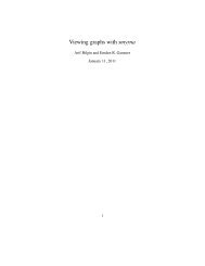
Figure 1 is an example graph in the DOT language. Line 1 gives the graph<br />
name and type. The lines that follow create nodes, edges, or sub<strong>graphs</strong>, and set<br />
attributes. Names of all these objects may be C identifiers, numbers, or quoted C<br />
strings. Quotes protect punctuation and white space.<br />
A node is created when its name first appears in the file. An edge is created<br />
when nodes are joined by the edge operator ->. In the example, line 2 makes<br />
edges from main to parse, and from parse to execute. Running <strong>dot</strong> on this file (call<br />
it graph1.<strong>dot</strong>)<br />
$ <strong>dot</strong> -Tps graph1.<strong>dot</strong> -o graph1.ps<br />
yields the drawing of Figure 2. The command line option -Tps selects PostScript<br />
(EPSF) output. graph1.ps may be printed, displayed by a PostScript viewer, or<br />
embedded in another document.<br />
It is often useful to adjust the representation or placement of nodes and edges<br />
in the layout. This is done by setting attributes of nodes, edges, or sub<strong>graphs</strong> in<br />
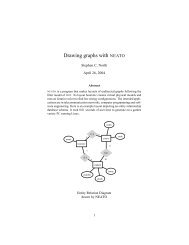
the input file. Attributes are name-value pairs of character strings. Figures 3 and 4<br />
illustrate some layout attributes. In the listing of Figure 3, line 2 sets the graph’s
<strong>dot</strong> User’s Manual, January 26, 2006 3<br />
1: digraph G {<br />
2: main -> parse -> execute;<br />
3: main -> init;<br />
4: main -> cleanup;<br />
5: execute -> make_string;<br />
6: execute -> printf<br />
7: init -> make_string;<br />
8: main -> printf;<br />
9: execute -> compare;<br />
10: }<br />
init<br />
Figure 1: Small graph<br />
parse<br />
main<br />
execute<br />
make_string compare<br />
cleanup<br />
printf<br />
Figure 2: <strong>Drawing</strong> of small graph
<strong>dot</strong> User’s Manual, January 26, 2006 4<br />
size to 4,4 (in inches). This attribute controls the size of the drawing; if the<br />
drawing is too large, it is scaled as necessary to fit.<br />
Node or edge attributes are set off in square brackets. In line 3, the node main<br />
is assigned shape box. The edge in line 4 is straightened by increasing its weight<br />
(the default is 1). The edge in line 6 is drawn as a <strong>dot</strong>ted line. Line 8 makes edges<br />
from execute to make string and printf. In line 10 the default edge color<br />
is set to red. This affects any edges created after this point in the file. Line 11<br />
makes a bold edge labeled 100 times. In line 12, node make_string is given<br />
a multi-line label. Line 13 changes the default node to be a box filled <strong>with</strong> a shade<br />
of blue. The node compare inherits these values.<br />
2 <strong>Drawing</strong> Attributes<br />
The complete list of attributes that affect graph drawing is summarized in Tables 1,<br />
2 and 3.<br />
2.1 Node Shapes<br />
Nodes are drawn, by default, <strong>with</strong> shape=ellipse, width=.75, height=.5<br />
and labeled by the node name. Other common shapes include box, circle,<br />
record and plaintext. A complete list of node shapes is given in Appendix E.<br />
The node shape plaintext is of particularly interest in that it draws a node <strong>with</strong>out<br />
any outline, an important convention in some kinds of diagrams. In cases where<br />
the graph structure is of main concern, and especially when the graph is moderately<br />
large, the point shape reduces nodes to display minimal content. When drawn, a<br />
node’s actual size is the greater of the requested size and the area needed for its text<br />
label, unless fixedsize=true, in which case the width and height values<br />
are enforced.<br />
Node shapes fall into two broad categories: polygon-based and record-based. 1<br />
All node shapes except record and Mrecord are considered polygonal, and<br />
are modeled by the number of sides (ellipses and circles being special cases), and<br />
a few other geometric properties. Some of these properties can be specified in<br />
a graph. If regular=true, the node is forced to be regular. The parameter<br />
peripheries sets the number of boundary curves drawn. For example, a doublecircle<br />
has peripheries=2. The orientation attribute specifies a clockwise<br />
rotation of the polygon, measured in degrees.<br />
1 There is a way to implement custom node shapes, using shape=epsf and the shapefile<br />
attribute, and relying on PostScript output. The details are beyond the scope of this user’s guide.<br />
Please contact the authors for further information.
<strong>dot</strong> User’s Manual, January 26, 2006 5<br />
1: digraph G {<br />
2: size ="4,4";<br />
3: main [shape=box]; /* this is a comment */<br />
4: main -> parse [weight=8];<br />
5: parse -> execute;<br />
6: main -> init [style=<strong>dot</strong>ted];<br />
7: main -> cleanup;<br />
8: execute -> { make_string; printf}<br />
9: init -> make_string;<br />
10: edge [color=red]; // so is this<br />
11: main -> printf [style=bold,label="100 times"];<br />
12: make_string [label="make a\nstring"];<br />
13: node [shape=box,style=filled,color=".7 .3 1.0"];<br />
14: execute -> compare;<br />
15: }<br />
printf<br />
Figure 3: Fancy graph<br />
100 times<br />
main<br />
parse<br />
execute<br />
compare<br />
init<br />
make a<br />
string<br />
cleanup<br />
Figure 4: <strong>Drawing</strong> of fancy graph
<strong>dot</strong> User’s Manual, January 26, 2006 6<br />
The shape polygon exposes all the polygonal parameters, and is useful for<br />
creating many shapes that are not predefined. In addition to the parameters regular,<br />
peripheries and orientation, mentioned above, polygons are parameterized<br />
by number of sides sides, skew and distortion. skew is a floating<br />
point number (usually between −1.0 and 1.0) that distorts the shape by slanting<br />
it from top-to-bottom, <strong>with</strong> positive values moving the top of the polygon to the<br />
right. Thus, skew can be used to turn a box into a parallelogram. distortion<br />
shrinks the polygon from top-to-bottom, <strong>with</strong> negative values causing the bottom<br />
to be larger than the top. distortion turns a box into a trapezoid. A variety of<br />
these polygonal attributes are illustrated in Figures 6 and 5.<br />
Record-based nodes form the other class of node shapes. These include the<br />
shapes record and Mrecord. The two are identical except that the latter has<br />
rounded corners. These nodes represent recursive lists of fields, which are drawn<br />
as alternating horizontal and vertical rows of boxes. The recursive structure is<br />
determined by the node’s label, which has the following schema:<br />
rlabel → field ( ’|’ field )*<br />
field → boxLabel | ’’ rlabel ’’<br />
boxLabel → [ ’’ ] [ string ]<br />
Literal braces, vertical bars and angle brackets must be escaped. Spaces are<br />
interpreted as separators between tokens, so they must be escaped if they are to<br />
appear literally in the text. The first string in a boxLabel gives a name to the field,<br />
and serves as a port name for the box (cf. Section 3.1). The second string is used<br />
as a label for the field; it may contain the same escape sequences as multi-line<br />
labels (cf. Section 2.2. The example of Figures 7 and 8 illustrates the use and some<br />
properties of records.<br />
2.2 Labels<br />
As mentioned above, the default node label is its name. Edges are unlabeled by<br />
default. Node and edge labels can be set explicitly using the label attribute as<br />
shown in Figure 4.<br />
Though it may be convenient to label nodes by name, at other times labels<br />
must be set explicitly. For example, in drawing a file directory tree, one might have<br />
several directories named src, but each one must have a unique node identifier.<br />
The inode number or full path name are suitable unique identifiers. Then the label<br />
of each node can be set to the file name <strong>with</strong>in its directory.
<strong>dot</strong> User’s Manual, January 26, 2006 7<br />
1: digraph G {<br />
2: a -> b -> c;<br />
3: b -> d;<br />
4: a [shape=polygon,sides=5,peripheries=3,color=lightblue,style=filled];<br />
5: c [shape=polygon,sides=4,skew=.4,label="hello world"]<br />
6: d [shape=invtriangle];<br />
7: e [shape=polygon,sides=4,distortion=.7];<br />
8: }<br />
Figure 5: Graph <strong>with</strong> polygonal shapes<br />
hello world d<br />
a<br />
b<br />
Figure 6: <strong>Drawing</strong> of polygonal node shapes<br />
e
<strong>dot</strong> User’s Manual, January 26, 2006 8<br />
1: digraph structs {<br />
2: node [shape=record];<br />
3: struct1 [shape=record,label=" left| mid\ dle| right"];<br />
4: struct2 [shape=record,label=" one| two"];<br />
5: struct3 [shape=record,label="hello\nworld |{ b |{c| d|e}| f}| g | h"];<br />
6: struct1 -> struct2;<br />
7: struct1 -> struct3;<br />
8: }<br />
one two<br />
Figure 7: Records <strong>with</strong> nested fields<br />
left mid dle right<br />
hello<br />
world<br />
b<br />
c d e<br />
Figure 8: <strong>Drawing</strong> of records<br />
f<br />
g h
<strong>dot</strong> User’s Manual, January 26, 2006 9<br />
Multi-line labels can be created by using the escape sequences \n, \l, \r to<br />
terminate lines that are centered, or left or right justified. 2<br />
Graphs and cluster sub<strong>graphs</strong> may also have labels. Graph labels appear, by<br />
default, centered below the graph. Setting labelloc=t centers the label above<br />
the graph. Cluster labels appear <strong>with</strong>in the enclosing rectangle, in the upper left<br />
corner. The value labelloc=b moves the label to the bottom of the rectangle.<br />
The setting labeljust=r moves the label to the right.<br />
The default font is 14-point Times-Roman, in black. Other font families,<br />
sizes and colors may be selected using the attributes fontname, fontsize and<br />
fontcolor. Font names should be compatible <strong>with</strong> the target interpreter. It is<br />
best to use only the standard font families Times, Helvetica, Courier or Symbol<br />
as these are guaranteed to work <strong>with</strong> any target graphics language. For example,<br />
Times-Italic, Times-Bold, and Courier are portable; AvanteGarde-<br />
DemiOblique isn’t.<br />
For bitmap output, such as GIF or JPG, <strong>dot</strong> relies on having these fonts available<br />
during layout. The fontpath attribute can specify a list of directories 3<br />
which should be searched for the font files. If this is not set, <strong>dot</strong> will use the<br />
DOTFONTPATH environment variable or, if this is not set, the GDFONTPATH<br />
environment variable. If none of these is set, <strong>dot</strong> uses a built-in list.<br />
Edge labels are positioned near the center of the edge. Usually, care is taken to<br />
prevent the edge label from overlapping edges and nodes. It can still be difficult,<br />
in a complex graph, to be certain which edge a label belongs to. If the decorate<br />
attribute is set to true, a line is drawn connecting the label to its edge. Sometimes<br />
avoiding collisions among edge labels and edges forces the drawing to be bigger<br />
than desired. If labelfloat=true, <strong>dot</strong> does not try to prevent such overlaps,<br />
allowing a more compact drawing.<br />
An edge can also specify additional labels, using headlabel and taillabel,<br />
which are be placed near the ends of the edge. The characteristics of these labels<br />
are specified using the attributes labelfontname, labelfontsize and<br />
labelfontcolor. These labels are placed near the intersection of the edge and<br />
the node and, as such, may interfere <strong>with</strong> them. To tune a drawing, the user can set<br />
the labelangle and labeldistance attributes. The former sets the angle,<br />
in degrees, which the label is rotated from the angle the edge makes incident <strong>with</strong><br />
the node. The latter sets a multiplicative scaling factor to adjust the distance that<br />
the label is from the node.<br />
2 The escape sequence \N is an internal symbol for node names.<br />
3 For Unix-based systems, this is a concatenated list of pathnames, separated by colons. For<br />
Windows-based systems, the pathnames are separated by semi-colons.
<strong>dot</strong> User’s Manual, January 26, 2006 10<br />
Name Default Values<br />
color black node shape color<br />
comment any string (format-dependent)<br />
distortion 0.0 node distortion for shape=polygon<br />
fillcolor lightgrey/black node fill color<br />
fixedsize false label text has no affect on node size<br />
fontcolor black type face color<br />
fontname Times-Roman font family<br />
fontsize 14 point size of label<br />
group name of node’s group<br />
height .5 height in inches<br />
label node name any string<br />
layer overlay range all, id or id:id<br />
orientation 0.0 node rotation angle<br />
peripheries shape-dependent number of node boundaries<br />
regular false force polygon to be regular<br />
shape ellipse node shape; see Section 2.1 and Appendix E<br />
shapefile external EPSF or SVG custom shape file<br />
sides 4 number of sides for shape=polygon<br />
skew 0.0 skewing of node for shape=polygon<br />
style graphics options, e.g. bold, <strong>dot</strong>ted,<br />
filled; cf. Section 2.3<br />
URL URL associated <strong>with</strong> node (format-dependent)<br />
width .75 width in inches<br />
z 0.0 z coordinate for VRML output<br />
Table 1: Node attributes
<strong>dot</strong> User’s Manual, January 26, 2006 11<br />
Name Default Values<br />
arrowhead normal style of arrowhead at head end<br />
arrowsize 1.0 scaling factor for arrowheads<br />
arrowtail normal style of arrowhead at tail end<br />
color black edge stroke color<br />
comment any string (format-dependent)<br />
constraint true use edge to affect node ranking<br />
decorate if set, draws a line connecting labels <strong>with</strong> their edges<br />
dir forward forward, back, both, or none<br />
fontcolor black type face color<br />
fontname Times-Roman font family<br />
fontsize 14 point size of label<br />
headlabel label placed near head of edge<br />
headport n,ne,e,se,s,sw,w,nw<br />
headURL URL attached to head label if output format is ismap<br />
label edge label<br />
labelangle -25.0 angle in degrees which head or tail label is rotated off edge<br />
labeldistance 1.0 scaling factor for distance of head or tail label from node<br />
labelfloat false lessen constraints on edge label placement<br />
labelfontcolor black type face color for head and tail labels<br />
labelfontname Times-Roman font family for head and tail labels<br />
labelfontsize 14 point size for head and tail labels<br />
layer overlay range all, id or id:id<br />
lhead name of cluster to use as head of edge<br />
ltail name of cluster to use as tail of edge<br />
minlen 1 minimum rank distance between head and tail<br />
samehead tag for head node; edge heads <strong>with</strong> the same tag are<br />
merged onto the same port<br />
sametail tag for tail node; edge tails <strong>with</strong> the same tag are merged<br />
onto the same port<br />
style graphics options, e.g. bold, <strong>dot</strong>ted, filled; cf.<br />
Section 2.3<br />
taillabel label placed near tail of edge<br />
tailport n,ne,e,se,s,sw,w,nw<br />
tailURL URL attached to tail label if output format is ismap<br />
weight 1 integer cost of stretching an edge<br />
Table 2: Edge attributes
<strong>dot</strong> User’s Manual, January 26, 2006 12<br />
Name Default Values<br />
bgcolor background color for drawing, plus initial fill color<br />
center false center drawing on page<br />
clusterrank local may be global or none<br />
color black for clusters, outline color, and fill color if fillcolor not defined<br />
comment any string (format-dependent)<br />
compound false allow edges between clusters<br />
concentrate false enables edge concentrators<br />
fillcolor black cluster fill color<br />
fontcolor black type face color<br />
fontname Times-Roman font family<br />
fontpath list of directories to search for fonts<br />
fontsize 14 point size of label<br />
label any string<br />
labeljust centered ”l” and ”r” for left- and right-justified cluster labels, respectively<br />
labelloc top ”t” and ”b” for top- and bottom-justified cluster labels, respectively<br />
layers id:id:id...<br />
margin .5 margin included in page, inches<br />
mclimit 1.0 scale factor for mincross iterations<br />
nodesep .25 separation between nodes, in inches.<br />
nslimit if set to f, bounds network simplex iterations by (f)(number of nodes)<br />
when setting x-coordinates<br />
nslimit1 if set to f, bounds network simplex iterations by (f)(number of nodes)<br />
when ranking nodes<br />
ordering if out out edge order is preserved<br />
orientation portrait if rotate is not used and the value is landscape, use landscape<br />
orientation<br />
page unit of pagination, e.g. "8.5,11"<br />
pagedir BL traversal order of pages<br />
quantum if quantum ¿ 0.0, node label dimensions will be rounded to integral<br />
multiples of quantum<br />
rank same, min, max, source or sink<br />
rankdir TB LR (left to right) or TB (top to bottom)<br />
ranksep .75 separation between ranks, in inches.<br />
ratio approximate aspect ratio desired, fill or auto<br />
remincross if true and there are multiple clusters, re-run crossing minimization<br />
rotate If 90, set orientation to landscape<br />
samplepoints 8 number of points used to represent ellipses and circles on output (cf.<br />
Appendix C<br />
searchsize 30 maximum edges <strong>with</strong> negative cut values to check when looking for a<br />
minimum one during network simplex<br />
size maximum drawing size, in inches<br />
style graphics options, e.g. filled for clusters<br />
URL URL associated <strong>with</strong> graph (format-dependent)<br />
Table 3: Graph attributes
<strong>dot</strong> User’s Manual, January 26, 2006 13<br />
2.3 Graphics Styles<br />
Nodes and edges can specify a color attribute, <strong>with</strong> black the default. This is the<br />
color used to draw the node’s shape or the edge. A color value can be a huesaturation-brightness<br />
triple (three floating point numbers between 0 and 1, separated<br />
by commas); one of the colors names listed in Appendix G (borrowed from<br />
some version of the X window system); or a red-green-blue (RGB) triple 4 (three<br />
hexadecimal number between 00 and FF, preceded by the character ’#’). Thus,<br />
the values "orchid", "0.8396,0.4862,0.8549" and #DA70D6 are three<br />
ways to specify the same color. The numerical forms are convenient for scripts or<br />
tools that automatically generate colors. Color name lookup is case-insensitive and<br />
ignores non-alphanumeric characters, so warmgrey and Warm_Grey are equivalent.<br />
We can offer a few hints regarding use of color in graph drawings. First, avoid<br />
using too many bright colors. A “rainbow effect” is confusing. It is better to<br />
choose a narrower range of colors, or to vary saturation along <strong>with</strong> hue. Second,<br />
when nodes are filled <strong>with</strong> dark or very saturated colors, labels seem to be<br />
more readable <strong>with</strong> fontcolor=white and fontname=Helvetica. (We<br />
also have PostScript functions for <strong>dot</strong> that create outline fonts from plain fonts.)<br />
Third, in certain output formats, you can define your own color space. For example,<br />
if using PostScript for output, you can redefine nodecolor, edgecolor,<br />
or graphcolor in a library file. Thus, to use RGB colors, place the following<br />
line in a file lib.ps.<br />
/nodecolor {setrgbcolor} bind def<br />
Use the -l command line option to load this file.<br />
<strong>dot</strong> -Tps -l lib.ps file.<strong>dot</strong> -o file.ps<br />
The style attribute controls miscellaneous graphics features of nodes and<br />
edges. This attribute is a comma-separated list of primitives <strong>with</strong> optional argument<br />
lists. The predefined primitives include solid, dashed, <strong>dot</strong>ted, bold<br />
and invis. The first four control line drawing in node boundaries and edges<br />
and have the obvious meaning. The value invis causes the node or edge to be<br />
left undrawn. The style for nodes can also include filled, diagonals and<br />
rounded. filled shades inside the node using the color fillcolor. If this<br />
is not set, the value of color is used. If this also is unset, light grey 5 is used as the<br />
4 A fourth form, RGBA, is also supported, which has the same format as RGB <strong>with</strong> an additional<br />
fourth hexadecimal number specifying alpha channel or transparency information.<br />
5 The default is black if the output format is MIF, or if the shape is point.
<strong>dot</strong> User’s Manual, January 26, 2006 14<br />
default. The diagonals style causes short diagonal lines to be drawn between<br />
pairs of sides near a vertex. The rounded style rounds polygonal corners.<br />
User-defined style primitives can be implemented as custom PostScript procedures.<br />
Such primitives are executed inside the gsave context of a graph, node,<br />
or edge, before any of its marks are drawn. The argument lists are translated to<br />
PostScript notation. For example, a node <strong>with</strong> style="setlinewidth(8)"<br />
is drawn <strong>with</strong> a thick outline. Here, setlinewidth is a PostScript built-in, but<br />
user-defined PostScript procedures are called the same way. The definition of these<br />
procedures can be given in a library file loaded using -l as shown above.<br />
Edges have a dir attribute to set arrowheads. dir may be forward (the<br />
default), back, both, or none. This refers only to where arrowheads are drawn,<br />
and does not change the underlying graph. For example, setting dir=back causes<br />
an arrowhead to be drawn at the tail and no arrowhead at the head, but it does not<br />
exchange the endpoints of the edge. The attributes arrowhead and arrowtail<br />
specify the style of arrowhead, if any, which is used at the head and tail ends of<br />
the edge. Allowed values are normal, inv, <strong>dot</strong>, inv<strong>dot</strong>, o<strong>dot</strong>, invo<strong>dot</strong><br />
and none (cf. Appendix F). The attribute arrowsize specifies a multiplicative<br />
factor affecting the size of any arrowhead drawn on the edge. For example,<br />
arrowsize=2.0 makes the arrow twice as long and twice as wide.<br />
In terms of style and color, clusters act somewhat like large box-shaped nodes,<br />
in that the cluster boundary is drawn using the cluster’s color attribute and, in<br />
general, the appearance of the cluster is affected the style, color and fillcolor<br />
attributes.<br />
If the root graph has a bgcolor attribute specified, this color is used as the<br />
background for the entire drawing, and also serves as the default fill color.<br />
2.4 <strong>Drawing</strong> Orientation, Size and Spacing<br />
Two attributes that play an important role in determining the size of a <strong>dot</strong> drawing<br />
are nodesep and ranksep. The first specifies the minimum distance, in inches,<br />
between two adjacent nodes on the same rank. The second deals <strong>with</strong> rank separation,<br />
which is the minimum vertical space between the bottoms of nodes in one<br />
rank and the tops of nodes in the next. The ranksep attribute sets the rank separation,<br />
in inches. Alternatively, one can have ranksep=equally. This guarantees<br />
that all of the ranks are equally spaced, as measured from the centers of nodes on<br />
adjacent ranks. In this case, the rank separation between two ranks is at least the<br />
default rank separation. As the two uses of ranksep are independent, both can<br />
be set at the same time. For example, ranksep="1.0 equally" causes ranks<br />
to be equally spaced, <strong>with</strong> a minimum rank separation of 1 inch.<br />
Often a drawing made <strong>with</strong> the default node sizes and separations is too big
<strong>dot</strong> User’s Manual, January 26, 2006 15<br />
for the target printer or for the space allowed for a figure in a document. There<br />
are several ways to try to deal <strong>with</strong> this problem. First, we will review how <strong>dot</strong><br />
computes the final layout size.<br />
A layout is initially made internally at its “natural” size, using default settings<br />
(unless ratio=compress was set, as described below). There is no bound on<br />
the size or aspect ratio of the drawing, so if the graph is large, the layout is also<br />
large. If you don’t specify size or ratio, then the natural size layout is printed.<br />
The easiest way to control the output size of the drawing is to set size="x,y"<br />
in the graph file (or on the command line using -G). This determines the size of the<br />
final layout. For example, size="7.5,10" fits on an 8.5x11 page (assuming<br />
the default page orientation) no matter how big the initial layout.<br />
ratio also affects layout size. There are a number of cases, depending on the<br />
settings of size and ratio.<br />
Case 1. ratio was not set. If the drawing already fits <strong>with</strong>in the given size,<br />
then nothing happens. Otherwise, the drawing is reduced uniformly enough to<br />
make the critical dimension fit.<br />
If ratio was set, there are four subcases.<br />
Case 2a. If ratio=x where x is a floating point number, then the drawing<br />
is scaled up in one dimension to achieve the requested ratio expressed as drawing<br />
height/width. For example, ratio=2.0 makes the drawing twice as high as it<br />
is wide. Then the layout is scaled using size as in Case 1.<br />
Case 2b. If ratio=fill and size=x, y was set, then the drawing is scaled<br />
up in one dimension to achieve the ratio y/x. Then scaling is performed as in Case<br />
1. The effect is that all of the bounding box given by size is filled.<br />
Case 2c. If ratio=compress and size=x, y was set, then the initial layout<br />
is compressed to attempt to fit it in the given bounding box. This trades off layout<br />
quality, balance and symmetry in order to pack the layout more tightly. Then<br />
scaling is performed as in Case 1.<br />
Case 2d. If ratio=auto and the page attribute is set and the graph cannot<br />
be drawn on a single page, then size is ignored and <strong>dot</strong> computes an “ideal” size.<br />
In particular, the size in a given dimension will be the smallest integral multiple<br />
of the page size in that dimension which is at least half the current size. The two<br />
dimensions are then scaled independently to the new size.<br />
If rotate=90 is set, or orientation=landscape, then the drawing is<br />
rotated 90 ◦ into landscape mode. The X axis of the layout would be along the Y<br />
axis of each page. This does not affect <strong>dot</strong>’s interpretation of size, ratio or<br />
page.<br />
At this point, if page is not set, then the final layout is produced as one page.<br />
If page=x, y is set, then the layout is printed as a sequence of pages which<br />
can be tiled or assembled into a mosaic. Common settings are page="8.5,11"
<strong>dot</strong> User’s Manual, January 26, 2006 16<br />
or page="11,17". These values refer to the full size of the physical device; the<br />
actual area used will be reduced by the margin settings. (For printer output, the<br />
default is 0.5 inches; for bitmap-output, the X and Y margins are 10 and 2 points,<br />
respectively.) For tiled layouts, it may be helpful to set smaller margins. This can<br />
be done by using the margin attribute. This can take a single number, used to set<br />
both margins, or two numbers separated by a comma to set the x and y margins<br />
separately. As usual, units are in inches. Although one can set margin=0, unfortunately,<br />
many bitmap printers have an internal hardware margin that cannot be<br />
overridden.<br />
The order in which pages are printed can be controlled by the pagedir attribute.<br />
Output is always done using a row-based or column-based ordering, and<br />
pagedir is set to a two-letter code specifying the major and minor directions. For<br />
example, the default is BL, specifying a bottom-to-top (B) major order and a leftto-right<br />
(L) minor order. Thus, the bottom row of pages is emitted first, from left<br />
to right, then the second row up, from left to right, and finishing <strong>with</strong> the top row,<br />
from left to right. The top-to-bottom order is represented by T and the right-to-left<br />
order by R.<br />
If center=true and the graph can be output on one page, using the default<br />
page size of 8.5 by 11 inches if page is not set, the graph is repositioned to be<br />
centered on that page.<br />
A common problem is that a large graph drawn at a small size yields unreadable<br />
node labels. To make larger labels, something has to give. There is a limit to the<br />
amount of readable text that can fit on one page. Often you can draw a smaller<br />
graph by extracting an interesting piece of the original graph before running <strong>dot</strong>.<br />
We have some tools that help <strong>with</strong> this.<br />
sccmap decompose the graph into strongly connected components<br />
tred compute transitive reduction (remove edges implied by transitivity)<br />
gvpr graph processor to select nodes or edges, and contract or remove the rest of<br />
the graph<br />
unflatten improve aspect ratio of trees by staggering the lengths of leaf edges<br />
With this in mind, here are some thing to try on a given graph:<br />
1. Increase the node fontsize.<br />
2. Use smaller ranksep and nodesep.<br />
3. Use ratio=auto.
<strong>dot</strong> User’s Manual, January 26, 2006 17<br />
4. Use ratio=compress and give a reasonable size.<br />
5. A sans serif font (such as Helvetica) may be more readable than Times when<br />
reduced.<br />
2.5 Node and Edge Placement<br />
Attributes in <strong>dot</strong> provide many ways to adjust the large-scale layout of nodes and<br />
edges, as well as fine-tune the drawing to meet the user’s needs and tastes. This<br />
section discusses these attributes 6 .<br />
Sometimes it is natural to make edges point from left to right instead of from<br />
top to bottom. If rankdir=LR in the top-level graph, the drawing is rotated in this<br />
way. TB (top to bottom) is the default. The mode rankdir=BT is useful for drawing<br />
upward-directed <strong>graphs</strong>. For completeness, one can also have rankdir=RL.<br />
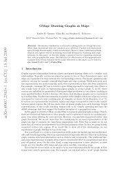
In <strong>graphs</strong> <strong>with</strong> time-lines, or in drawings that emphasize source and sink nodes,<br />
you may need to constrain rank assignments. The rank of a subgraph may be set<br />
to same, min, source, max or sink. A value same causes all the nodes in the<br />
subgraph to occur on the same rank. If set to min, all the nodes in the subgraph<br />
are guaranteed to be on a rank at least as small as any other node in the layout 7 .<br />
This can be made strict by setting rank=source, which forces the nodes in the<br />
subgraph to be on some rank strictly smaller than the rank of any other nodes<br />
(except those also specified by min or source sub<strong>graphs</strong>). The values max or<br />
sink play an analogous role for the maximum rank. Note that these constraints<br />
induce equivalence classes of nodes. If one subgraph forces nodes A and B to be<br />
on the same rank, and another subgraph forces nodes C and B to share a rank, then<br />
all nodes in both sub<strong>graphs</strong> must be drawn on the same rank. Figures 9 and 10<br />
illustrate using sub<strong>graphs</strong> for controlling rank assignment.<br />
In some <strong>graphs</strong>, the left-to-right ordering of nodes is important. If a subgraph<br />
has ordering=out, then out-edges <strong>with</strong>in the subgraph that have the same tail<br />
node wll fan-out from left to right in their order of creation. (Also note that flat<br />
edges involving the head nodes can potentially interfere <strong>with</strong> their ordering.)<br />
There are many ways to fine-tune the layout of nodes and edges. For example,<br />
if the nodes of an edge both have the same group attribute, <strong>dot</strong> tries to keep<br />
the edge straight and avoid having other edges cross it. The weight of an edge<br />
provides another way to keep edges straight. An edge’s weight suggests some<br />
measure of an edge’s importance; thus, the heavier the weight, the closer together<br />
6 For completeness, we note that <strong>dot</strong> also provides access to various parameters which play technical<br />
roles in the layout algorithms. These include mclimit, nslimit, nslimit1, remincross<br />
and searchsize.<br />
7 Recall that the minimum rank occurs at the top of a drawing.
<strong>dot</strong> User’s Manual, January 26, 2006 18<br />
digraph asde91 {<br />
ranksep=.75; size = "7.5,7.5";<br />
}<br />
{<br />
}<br />
node [shape=plaintext, fontsize=16];<br />
/* the time-line graph */<br />
past -> 1978 -> 1980 -> 1982 -> 1983 -> 1985 -> 1986 -><br />
1987 -> 1988 -> 1989 -> 1990 -> "future";<br />
/* ancestor programs */<br />
"Bourne sh"; "make"; "SCCS"; "yacc"; "cron"; "Reiser cpp";<br />
"Cshell"; "emacs"; "build"; "vi"; ""; "RCS"; "C*";<br />
{ rank = same;<br />
"Software IS"; "Configuration Mgt"; "Architecture & Libraries";<br />
"Process";<br />
};<br />
node [shape=box];<br />
{ rank = same; "past"; "SCCS"; "make"; "Bourne sh"; "yacc"; "cron"; }<br />
{ rank = same; 1978; "Reiser cpp"; "Cshell"; }<br />
{ rank = same; 1980; "build"; "emacs"; "vi"; }<br />
{ rank = same; 1982; "RCS"; ""; "IMX"; "SYNED"; }<br />
{ rank = same; 1983; "ksh"; "IFS"; "TTU"; }<br />
{ rank = same; 1985; "nmake"; "Peggy"; }<br />
{ rank = same; 1986; "C*"; "ncpp"; "ksh-i"; ""; "PG2"; }<br />
{ rank = same; 1987; "Ansi cpp"; "nmake 2.0"; "3D File System"; "fdelta";<br />
"DAG"; "CSAS";}<br />
{ rank = same; 1988; "CIA"; "SBCS"; "ksh-88"; "PEGASUS/PML"; "PAX";<br />
"backtalk"; }<br />
{ rank = same; 1989; "CIA++"; "APP"; "SHIP"; "DataShare"; "ryacc";<br />
"Mosaic"; }<br />
{ rank = same; 1990; "libft"; "CoShell"; "DIA"; "IFS-i"; "kyacc"; "sfio";<br />
"yeast"; "ML-X"; "DOT"; }<br />
{ rank = same; "future"; "Adv. Software Technology"; }<br />
"PEGASUS/PML" -> "ML-X";<br />
"SCCS" -> "nmake";<br />
"SCCS" -> "3D File System";<br />
"SCCS" -> "RCS";<br />
"make" -> "nmake";<br />
"make" -> "build";<br />
.<br />
.<br />
.<br />
Figure 9: Graph <strong>with</strong> constrained ranks
past<br />
1978<br />
1980<br />
1982<br />
1983<br />
1985<br />
1986<br />
1987<br />
1988<br />
1989<br />
1990<br />
future<br />
<strong>dot</strong> User’s Manual, January 26, 2006 19<br />
DAG<br />
DOT<br />
CIA++<br />
C*<br />
CSAS<br />
CIA<br />
DIA<br />
Software IS<br />
APP<br />
libft<br />
RCS<br />
Ansi cpp<br />
Reiser cpp<br />
ncpp<br />
SBCS<br />
fdelta<br />
SCCS<br />
PAX<br />
nmake<br />
make<br />
3D File System<br />
build<br />
<br />
<br />
nmake 2.0<br />
CoShell<br />
vi<br />
Bourne sh<br />
Cshell<br />
ksh<br />
ksh-i<br />
ksh-88<br />
Adv. Software Technology<br />
sfio<br />
emacs<br />
IFS<br />
IFS-i<br />
PEGASUS/PML<br />
SYNED<br />
Configuration Mgt Architecture & Libraries Process<br />
Peggy<br />
backtalk<br />
SHIP DataShare<br />
ML-X<br />
Figure 10: <strong>Drawing</strong> <strong>with</strong> constrained ranks<br />
kyacc<br />
ryacc<br />
IMX<br />
TTU<br />
PG2<br />
yacc<br />
Mosaic<br />
cron<br />
yeast
<strong>dot</strong> User’s Manual, January 26, 2006 20<br />
its nodes should be. <strong>dot</strong> causes edges <strong>with</strong> heavier weights to be drawn shorter and<br />
straighter.<br />
Edge weights also play a role when nodes are constrained to the same rank.<br />
Edges <strong>with</strong> non-zero weight between these nodes are aimed across the rank in<br />
the same direction (left-to-right, or top-to-bottom in a rotated drawing) as far as<br />
possible. This fact may be exploited to adjust node ordering by placing invisible<br />
edges (style="invis") where needed.<br />
The end points of edges adjacent to the same node can be constrained using the<br />
samehead and sametail attributes. Specifically, all edges <strong>with</strong> the same head<br />
and the same value of samehead are constrained to intersect the head node at the<br />
same point. The analogous property holds for tail nodes and sametail.<br />
During rank assignment, the head node of an edge is constrained to be on a<br />
higher rank than the tail node. If the edge has constraint=false, however,<br />
this requirement is not enforced.<br />
In certain circumstances, the user may desire that the end points of an edge<br />
never get too close. This can be obtained by setting the edge’s minlen attribute.<br />
This defines the minimum difference between the ranks of the head and tail. For<br />
example, if minlen=2, there will always be at least one intervening rank between<br />
the head and tail. Note that this is not concerned <strong>with</strong> the geometric distance between<br />
the two nodes.<br />
Fine-tuning should be approached cautiously. <strong>dot</strong> works best when it can<br />
makes a layout <strong>with</strong>out much “help” or interference in its placement of individual<br />
nodes and edges. Layouts can be adjusted somewhat by increasing the weight of<br />
certain edges, or by creating invisible edges or nodes using style=invis, and<br />
sometimes even by rearranging the order of nodes and edges in the file. But this can<br />
backfire because the layouts are not necessarily stable <strong>with</strong> respect to changes in<br />
the input graph. One last adjustment can invalidate all previous changes and make<br />
a very bad drawing. A future project we have in mind is to combine the mathematical<br />
layout techniques of <strong>dot</strong> <strong>with</strong> an interactive front-end that allows user-defined<br />
hints and constraints.<br />
3 Advanced Features<br />
3.1 Node Ports<br />
A node port is a point where edges can attach to a node. (When an edge is not<br />
attached to a port, it is aimed at the node’s center and the edge is clipped at the<br />
node’s boundary.)<br />
Simple ports can be specified by using the headport and tailport attributes.<br />
These can be assigned one of the 8 compass points "n", "ne", "e",
<strong>dot</strong> User’s Manual, January 26, 2006 21<br />
"se", "s", "sw", "w" or "nw". The end of the node will then be aimed at that<br />
position on the node. Thus, if tailport=se, the edge will connect to the tail<br />
node at its southeast “corner”.<br />
Nodes <strong>with</strong> a record shape use the record structure to define ports. As noted<br />
above, this shape represents a record as recursive lists of boxes. If a box defines<br />
a port name, by using the construct < port name > in the box label, the center<br />
of the box can be used a port. (By default, the edge is clipped to the box’s<br />
boundary.) This is done by modifying the node name <strong>with</strong> the port name, using the<br />
syntax node name:port name, as part of an edge declaration. Figure 11 illustrates<br />
the declaration and use of port names in record nodes, <strong>with</strong> the resulting drawing<br />
shown in Figure 12.<br />
DISCLAIMER: At present, simple ports don’t work as advertised, even<br />
when they should. There is also the case where we might not want them to<br />
work, e.g., when the tailport=n and the headport=s. Finally, in theory, <strong>dot</strong><br />
should be able to allow both types of ports on an edge, since the notions are<br />
orthogonal. There is still the question as to whether the two syntaxes could<br />
be combined, i.e., treat the compass points as reserved port names, and allow<br />
nodename:portname:compassname.<br />
Figures 13 and 14 give another example of the use of record nodes and ports.<br />
This repeats the example of Figures 7 and 8 but now using ports as connectors<br />
for edges. Note that records sometimes look better if their input height is set to a<br />
small value, so the text labels dominate the actual size, as illustrated in Figure 11.<br />
Otherwise the default node size (.75 by .5) is assumed, as in Figure 14. The<br />
example of Figures 15 and 16 uses left-to-right drawing in a layout of a hash table.<br />
3.2 Clusters<br />
A cluster is a subgraph placed in its own distinct rectangle of the layout. A subgraph<br />
is recognized as a cluster when its name has the prefix cluster. (If the<br />
top-level graph has clusterrank=none, this special processing is turned off).<br />
Labels, font characteristics and the labelloc attribute can be set as they would<br />
be for the top-level graph, though cluster labels appear above the graph by default.<br />
For clusters, the label is left-justified by default; if labeljust="r", the label is<br />
right-justified. The color attribute specifies the color of the enclosing rectangle.<br />
In addition, clusters may have style="filled", in which case the rectangle<br />
is filled <strong>with</strong> the color specified by fillcolor before the cluster is drawn. (If<br />
fillcolor is not specified, the cluster’s color attribute is used.)<br />
Clusters are drawn by a recursive technique that computes a rank assignment<br />
and internal ordering of nodes <strong>with</strong>in clusters. Figure 17 through 19 are cluster
<strong>dot</strong> User’s Manual, January 26, 2006 22<br />
1: digraph g {<br />
2: node [shape = record,height=.1];<br />
3: node0[label = " | G| "];<br />
4: node1[label = " | E| "];<br />
5: node2[label = " | B| "];<br />
6: node3[label = " | F| "];<br />
7: node4[label = " | R| "];<br />
8: node5[label = " | H| "];<br />
9: node6[label = " | Y| "];<br />
10: node7[label = " | A| "];<br />
11: node8[label = " | C| "];<br />
12: "node0":f2 -> "node4":f1;<br />
13: "node0":f0 -> "node1":f1;<br />
14: "node1":f0 -> "node2":f1;<br />
15: "node1":f2 -> "node3":f1;<br />
16: "node2":f2 -> "node8":f1;<br />
17: "node2":f0 -> "node7":f1;<br />
18: "node4":f2 -> "node6":f1;<br />
19: "node4":f0 -> "node5":f1;<br />
20: }<br />
Figure 11: Binary search tree using records<br />
B F<br />
A C<br />
G<br />
E R<br />
H Y<br />
Figure 12: <strong>Drawing</strong> of binary search tree
<strong>dot</strong> User’s Manual, January 26, 2006 23<br />
1: digraph structs {<br />
2: node [shape=record];<br />
3: struct1 [shape=record,label=" left| middle| right"];<br />
4: struct2 [shape=record,label=" one| two"];<br />
5: struct3 [shape=record,label="hello\nworld |{ b |{c| d|e}| f}| g | h"];<br />
6: struct1:f1 -> struct2:f0;<br />
7: struct1:f2 -> struct3:here;<br />
8: }<br />
Figure 13: Records <strong>with</strong> nested fields (revisited)<br />
left middle right<br />
one two<br />
hello<br />
world<br />
b<br />
c d e<br />
Figure 14: <strong>Drawing</strong> of records (revisited)<br />
f<br />
g h
<strong>dot</strong> User’s Manual, January 26, 2006 24<br />
1: digraph G {<br />
2: nodesep=.05;<br />
3: rankdir=LR;<br />
4: node [shape=record,width=.1,height=.1];<br />
5:<br />
6: node0 [label = " | | | | | | | ",height=2.5];<br />
7: node [width = 1.5];<br />
8: node1 [label = "{ n14 | 719 | }"];<br />
9: node2 [label = "{ a1 | 805 | }"];<br />
10: node3 [label = "{ i9 | 718 | }"];<br />
11: node4 [label = "{ e5 | 989 | }"];<br />
12: node5 [label = "{ t20 | 959 | }"] ;<br />
13: node6 [label = "{ o15 | 794 | }"] ;<br />
14: node7 [label = "{ s19 | 659 | }"] ;<br />
15:<br />
16: node0:f0 -> node1:n;<br />
17: node0:f1 -> node2:n;<br />
18: node0:f2 -> node3:n;<br />
19: node0:f5 -> node4:n;<br />
20: node0:f6 -> node5:n;<br />
21: node2:p -> node6:n;<br />
22: node4:p -> node7:n;<br />
23: }<br />
Figure 15: Hash table graph file<br />
n14 719<br />
a1 805<br />
i9 718<br />
e5 989<br />
t20 959<br />
o15 794<br />
s19 659<br />
Figure 16: <strong>Drawing</strong> of hash table
<strong>dot</strong> User’s Manual, January 26, 2006 25<br />
layouts and the corresponding graph files.
<strong>dot</strong> User’s Manual, January 26, 2006 26<br />
digraph G {<br />
subgraph cluster0 {<br />
node [style=filled,color=white];<br />
style=filled;<br />
color=lightgrey;<br />
a0 -> a1 -> a2 -> a3;<br />
label = "process #1";<br />
}<br />
}<br />
subgraph cluster1 {<br />
node [style=filled];<br />
b0 -> b1 -> b2 -> b3;<br />
label = "process #2";<br />
color=blue<br />
}<br />
start -> a0;<br />
start -> b0;<br />
a1 -> b3;<br />
b2 -> a3;<br />
a3 -> a0;<br />
a3 -> end;<br />
b3 -> end;<br />
start [shape=Mdiamond];<br />
end [shape=Msquare];<br />
process #1 process #2<br />
a0<br />
a1<br />
a2<br />
a3<br />
start<br />
end<br />
Figure 17: Process diagram <strong>with</strong> clusters<br />
b0<br />
b1<br />
b3<br />
b2
<strong>dot</strong> User’s Manual, January 26, 2006 27<br />
If the top-level graph has the compound attribute set to true, <strong>dot</strong> will allow<br />
edges connecting nodes and clusters. This is accomplished by an edge defining<br />
an lhead or ltail attribute. The value of these attributes must be the name of<br />
a cluster containing the head or tail node, respectively. In this case, the edge is<br />
clipped at the cluster boundary. All other edge attributes, such as arrowhead<br />
or dir, are applied to the truncated edge. For example, Figure 20 shows a graph<br />
using the compound attribute and the resulting diagram.<br />
3.3 Concentrators<br />
Setting concentrate=true on the top-level graph enables an edge merging<br />
technique to reduce clutter in dense layouts. Edges are merged when they run<br />
parallel, have a common endpoint and have length greater than 1. A beneficial<br />
side-effect in fixed-sized layouts is that removal of these edges often permits larger,<br />
more readable labels. While concentrators in <strong>dot</strong> look somewhat like Newbery’s<br />
[New89], they are found by searching the edges in the layout, not by detecting<br />
complete bipartite <strong>graphs</strong> in the underlying graph. Thus the <strong>dot</strong> approach runs<br />
much faster but doesn’t collapse as many edges as Newbery’s algorithm.<br />
4 Command Line Options<br />
By default, <strong>dot</strong> operates in filter mode, reading a graph from stdin, and writing<br />
the graph on stdout in the DOT format <strong>with</strong> layout attributes appended. <strong>dot</strong><br />
supports a variety of command-line options:<br />
-Tformat sets the format of the output. Allowed values for format are:<br />
canon Prettyprint input; no layout is done.<br />
<strong>dot</strong> Attributed DOT. Prints input <strong>with</strong> layout information attached as attributes,<br />
cf. Appendix C.<br />
fig FIG output.<br />
gd GD format. This is the internal format used by the GD Graphics Library. An<br />
alternate format is gd2.<br />
gif GIF output.<br />
hpgl HP-GL/2 vector graphic printer language for HP wide bed plotters.<br />
imap Produces map files for server-side image maps. This can be combined <strong>with</strong><br />
a graphical form of the output, e.g., using -Tgif or -Tjpg, in web pages
<strong>dot</strong> User’s Manual, January 26, 2006 28<br />
1:digraph G {<br />
2: size="8,6"; ratio=fill; node[fontsize=24];<br />
3:<br />
4: ciafan->computefan; fan->increment; computefan->fan; stringdup->fatal;<br />
5: main->exit; main->interp_err; main->ciafan; main->fatal; main->malloc;<br />
6: main->strcpy; main->getopt; main->init_index; main->strlen; fan->fatal;<br />
7: fan->ref; fan->interp_err; ciafan->def; fan->free; computefan->stdprintf;<br />
8: computefan->get_sym_fields; fan->exit; fan->malloc; increment->strcmp;<br />
9: computefan->malloc; fan->stdsprintf; fan->strlen; computefan->strcmp;<br />
10: computefan->realloc; computefan->strlen; debug->sfprintf; debug->strcat;<br />
11: stringdup->malloc; fatal->sfprintf; stringdup->strcpy; stringdup->strlen;<br />
12: fatal->exit;<br />
13:<br />
14: subgraph "cluster_error.h" { label="error.h"; interp_err; }<br />
15:<br />
16: subgraph "cluster_sfio.h" { label="sfio.h"; sfprintf; }<br />
17:<br />
18: subgraph "cluster_ciafan.c" { label="ciafan.c"; ciafan; computefan;<br />
19: increment; }<br />
20:<br />
21: subgraph "cluster_util.c" { label="util.c"; stringdup; fatal; debug; }<br />
22:<br />
23: subgraph "cluster_query.h" { label="query.h"; ref; def; }<br />
24:<br />
25: subgraph "cluster_field.h" { get_sym_fields; }<br />
26:<br />
27: subgraph "cluster_stdio.h" { label="stdio.h"; stdprintf; stdsprintf; }<br />
28:<br />
29: subgraph "cluster_" { getopt; }<br />
30:<br />
31: subgraph "cluster_stdlib.h" { label="stdlib.h"; exit; malloc; free; realloc; }<br />
32:<br />
33: subgraph "cluster_main.c" { main; }<br />
34:<br />
35: subgraph "cluster_index.h" { init_index; }<br />
36:<br />
37: subgraph "cluster_string.h" { label="string.h"; strcpy; strlen; strcmp; strcat; }<br />
38:}<br />
Figure 18: Call graph file
strcat<br />
<strong>dot</strong> User’s Manual, January 26, 2006 29<br />
string.h<br />
debug<br />
util.c<br />
stringdup<br />
fatal<br />
getopt init_index<br />
sfio.h<br />
increment<br />
ciafan.c<br />
ciafan<br />
computefan def<br />
query.h<br />
fan<br />
stdio.h stdlib.h<br />
strcpy strlen strcmp sfprintf get_sym_fields stdprintf stdsprintf realloc<br />
main<br />
Figure 19: Call graph <strong>with</strong> labeled clusters<br />
ref<br />
malloc<br />
exit<br />
error.h<br />
interp_err<br />
free
<strong>dot</strong> User’s Manual, January 26, 2006 30<br />
digraph G {<br />
compound=true;<br />
subgraph cluster0 {<br />
a -> b;<br />
a -> c;<br />
b -> d;<br />
c -> d;<br />
}<br />
subgraph cluster1 {<br />
e -> g;<br />
e -> f;<br />
}<br />
b -> f [lhead=cluster1];<br />
d -> e;<br />
c -> g [ltail=cluster0,<br />
lhead=cluster1];<br />
c -> e [ltail=cluster0];<br />
d -> h;<br />
}<br />
Figure 20: Graph <strong>with</strong> edges on clusters<br />
h<br />
a<br />
b c<br />
d<br />
e<br />
f<br />
g
<strong>dot</strong> User’s Manual, January 26, 2006 31<br />
to attach links to nodes and edges. The format ismap is a predecessor of<br />
the imap format.<br />
cmap Produces HTML map files for client-side image maps.<br />
mif FrameMaker MIF format. In this format, <strong>graphs</strong> can be loaded into FrameMaker<br />
and edited manually. MIF is limited to 8 basic colors.<br />
mp MetaPost output.<br />
pcl PCL-5 output for HP laser writers.<br />
pic PIC output.<br />
plain Simple, line-based ASCII format. Appendix B describes this output. An<br />
alternate format is plain-ext, which provides port names on the head and<br />
tail nodes of edges.<br />
png PNG (Portable Network Graphics) output.<br />
ps PostScript (EPSF) output.<br />
ps2 PostScript (EPSF) output <strong>with</strong> PDF annotations. It is assumed that this output<br />
will be distilled into PDF.<br />
svg SVG output. The alternate form svgz produces compressed SVG.<br />
vrml VRML output.<br />
vtx VTX format for r Confluents’s Visual Thought.<br />
wbmp Wireless BitMap (WBMP) format.<br />
-Gname=value sets a graph attribute default value. Often it is convenient to set<br />
size, pagination, and related values on the command line rather than in the graph<br />
file. The analogous flags -N or -E set default node or edge attributes. Note that<br />
file contents override command line arguments.<br />
-llibfile specifies a device-dependent graphics library file. Multiple libraries<br />
may be given. These names are passed to the code generator at the beginning of<br />
output.<br />
-ooutfile writes output into file outfile.<br />
-v requests verbose output. In processing large layouts, the verbose messages<br />
may give some estimate of <strong>dot</strong>’s progress.<br />
-V prints the version number and exits.
<strong>dot</strong> User’s Manual, January 26, 2006 32<br />
5 Miscellaneous<br />
In the top-level graph heading, a graph may be declared a strict digraph.<br />
This forbids the creation of self-arcs and multi-edges; they are ignored in the input<br />
file.<br />
Nodes, edges and <strong>graphs</strong> may have a URL attribute. In certain output formats<br />
(ps2, imap, ismap, cmap, or svg), this information is integrated in the output<br />
so that nodes, edges and clusters become active links when displayed <strong>with</strong><br />
the appropriate tools. Typically, URLs attached to top-level <strong>graphs</strong> serve as base<br />
URLs, supporting relative URLs on components. When the output format is imap,<br />
or cmap, a similar processing takes place <strong>with</strong> the headURL and tailURL attributes.<br />
For certain formats (ps, fig, mif, mp, vtx or svg), comment attributes<br />
can be used to embed human-readable notations in the output.<br />
6 Conclusions<br />
<strong>dot</strong> produces pleasing hierarchical drawings and can be applied in many settings.<br />
Since the basic algorithms of <strong>dot</strong> work well, we have a good basis for further<br />
research into problems such as methods for drawing large <strong>graphs</strong> and on-line<br />
(animated) graph drawing.<br />
7 Acknowledgments<br />
We thank Phong Vo for his advice about graph drawing algorithms and programming.<br />
The graph library uses Phong’s splay tree dictionary library. Also, the users<br />
of dag, the predecessor of <strong>dot</strong>, gave us many good suggestions. Guy Jacobson<br />
and and Randy Hackbarth reviewed earlier drafts of this manual, and Emden contributed<br />
substantially to the current revision. John Ellson wrote the generalized<br />
polygon shape and spent considerable effort to make it robust and efficient. He<br />
also wrote the GIF and ISMAP generators and other tools to bring graphviz to the<br />
web.
<strong>dot</strong> User’s Manual, January 26, 2006 33<br />
References<br />
[Car80] M. Carpano. Automatic display of hierarchized <strong>graphs</strong> for computer<br />
aided decision analysis. IEEE Transactions on Software Engineering,<br />
SE-12(4):538–546, April 1980.<br />
[GKNV93] Emden R. Gansner, Eleftherios Koutsofios, Stephen C. North, and<br />
Kiem-Phong Vo. A Technique for <strong>Drawing</strong> Directed Graphs. IEEE<br />
Trans. Sofware Eng., 19(3):214–230, May 1993.<br />
[New89] Frances J. Newbery. Edge Concentration: A Method for Clustering<br />
Directed Graphs. In 2nd International Workshop on Software Configuration<br />
Management, pages 76–85, October 1989. Published as<br />
ACM SIGSOFT Software Engineering Notes, vol. 17, no. 7, November<br />
1989.<br />
[Nor92] Stephen C. North. Neato User’s Guide. Technical Report 59113-<br />
921014-14TM, AT&T Bell Laboratories, Murray Hill, NJ, 1992.<br />
[STT81] K. Sugiyama, S. Tagawa, and M. Toda. Methods for Visual Understanding<br />
of Hierarchical System Structures. IEEE Transactions on<br />
Systems, Man, and Cybernetics, SMC-11(2):109–125, February 1981.<br />
[War77] John Warfield. Crossing Theory and Hierarchy Mapping. IEEE Transactions<br />
on Systems, Man, and Cybernetics, SMC-7(7):505–523, July<br />
1977.
<strong>dot</strong> User’s Manual, January 26, 2006 34<br />
A Graph File Grammar<br />
The following is an abstract grammar for the DOT language. Terminals are shown<br />
in bold font and nonterminals in italics. Literal characters are given in single<br />
quotes. Parentheses ( and ) indicate grouping when needed. Square brackets [<br />
and ] enclose optional items. Vertical bars | separate alternatives.<br />
graph → [strict] (digraph | graph) id ’{’ stmt-list ’}’<br />
stmt-list → [stmt [’;’] [stmt-list ] ]<br />
stmt → attr-stmt | node-stmt | edge-stmt | subgraph | id ’=’ id<br />
attr-stmt → (graph | node | edge) attr-list<br />
attr-list → ’[’ [a-list ] ’]’ [attr-list]<br />
a-list → id ’=’ id [’,’] [a-list]<br />
node-stmt → node-id [attr-list]<br />
node-id → id [port]<br />
port → port-location [port-angle] | port-angle [port-location]<br />
port-location → ’:’ id | ’:’ ’(’ id ’,’ id ’)’<br />
port-angle → ’@’ id<br />
edge-stmt → (node-id | subgraph) edgeRHS [attr-list]<br />
edgeRHS → edgeop (node-id | subgraph) [edgeRHS]<br />
subgraph → [subgraph id] ’{’ stmt-list ’}’ | subgraph id<br />
An id is any alphanumeric string not beginning <strong>with</strong> a digit, but possibly including<br />
underscores; or a number; or any quoted string possibly containing escaped<br />
quotes.<br />
An edgeop is -> in directed <strong>graphs</strong> and -- in undirected <strong>graphs</strong>.<br />
The language supports C++-style comments: /* */ and //.<br />
Semicolons aid readability but are not required except in the rare case that a<br />
named subgraph <strong>with</strong> no body immediate precedes an anonymous subgraph, because<br />
under precedence rules this sequence is parsed as a subgraph <strong>with</strong> a heading<br />
and a body.<br />
Complex attribute values may contain characters, such as commas and white<br />
space, which are used in parsing the DOT language. To avoid getting a parsing<br />
error, such values need to be enclosed in double quotes.
<strong>dot</strong> User’s Manual, January 26, 2006 35<br />
B Plain Output File Format (-Tplain)<br />
The “plain” output format of <strong>dot</strong> lists node and edge information in a simple, lineoriented<br />
style which is easy to parse by front-end components. All coordinates and<br />
lengths are unscaled and in inches.<br />
The first line is:<br />
graph scalefactor width height<br />
The width and height values give the width and the height of the drawing; the<br />
lower-left corner of the drawing is at the origin. The scalefactor indicates how<br />
much to scale all coordinates in the final drawing.<br />
The next group of lines lists the nodes in the format:<br />
node name x y xsize ysize label style shape color fillcolor<br />
The name is a unique identifier. If it contains whitespace or punctuation, it is<br />
quoted. The x and y values give the coordinates of the center of the node; the width<br />
and height give the width and the height. The remaining parameters provide the<br />
node’s label, style, shape, color and fillcolor attributes, respectively.<br />
If the node does not have a style attribute, "solid" is used.<br />
The next group of lines lists edges:<br />
edge tail head n x1 y1 x2 y2 . . . xn yn [ label lx ly ] style color<br />
n is the number of coordinate pairs that follow as B-spline control points. If the<br />
edge is labeled, then the label text and coordinates are listed next. The edge description<br />
is completed by the edge’s style and color. As <strong>with</strong> nodes, if a<br />
style is not defined, "solid" is used.<br />
The last line is always:<br />
stop
<strong>dot</strong> User’s Manual, January 26, 2006 36<br />
C Attributed DOT Format (-T<strong>dot</strong>)<br />
This is the default output format. It reproduces the input, along <strong>with</strong> layout information<br />
for the graph. Coordinate values increase up and to the right. Positions<br />
are represented by two integers separated by a comma, representing the X and Y<br />
coordinates of the location specified in points (1/72 of an inch). A position refers<br />
to the center of its associated object. Lengths are given in inches.<br />
A bb attribute is attached to the graph, specifying the bounding box of the<br />
drawing. If the graph has a label, its position is specified by the lp attribute.<br />
Each node gets pos, width and height attributes. If the node is a record,<br />
the record rectangles are given in the rects attribute. If the node is polygonal<br />
and the vertices attribute is defined in the input graph, this attribute contains<br />
the vertices of the node. The number of points produced for circles and ellipses is<br />
governed by the samplepoints attribute.<br />
Every edge is assigned a pos attribute, which consists of a list of 3n + 1<br />
locations. These are B-spline control points: points p0, p1, p2, p3 are the first Bezier<br />
spline, p3, p4, p5, p6 are the second, etc. Currently, edge points are listed top-tobottom<br />
(or left-to-right) regardless of the orientation of the edge. This may change.<br />
In the pos attribute, the list of control points might be preceded by a start<br />
point ps and/or an end point pe. These have the usual position representation <strong>with</strong> a<br />
"s," or "e," prefix, respectively. A start point is present if there is an arrow at p0.<br />
In this case, the arrow is from p0 to ps, where ps is actually on the node’s boundary.<br />
The length and direction of the arrowhead is given by the vector (ps − p0). If there<br />
is no arrow, p0 is on the node’s boundary. Similarly, the point pe designates an<br />
arrow at the other end of the edge, connecting to the last spline point.<br />
If the edge has a label, the label position is given in lp.
<strong>dot</strong> User’s Manual, January 26, 2006 37<br />
D Layers<br />
<strong>dot</strong> has a feature for drawing parts of a single diagram on a sequence of overlapping<br />
“layers.” Typically the layers are overhead transparencies. To activate this feature,<br />
one must set the top-level graph’s layers attribute to a list of identifiers. A node<br />
or edge can then be assigned to a layer or range of layers using its layer attribute..<br />
all is a reserved name for all layers (and can be used at either end of a range, e.g<br />
design:all or all:code). For example:<br />
layers = "spec:design:code:debug:ship";<br />
node90 [layer = "code"];<br />
node91 [layer = "design:debug"];<br />
node90 -> node91 [layer = "all"];<br />
node92 [layer = "all:code"];<br />
In this graph, node91 is in layers design, code and debug, while node92 is<br />
in layers spec, design and code.<br />
In a layered graph, if a node or edge has no layer assignment, but incident<br />
edges or nodes do, then its layer specification is inferred from these. To change the<br />
default so that nodes and edges <strong>with</strong> no layer appear on all layers, insert near the<br />
beginning of the graph file:<br />
node [layer=all];<br />
edge [layer=all];<br />
There is currently no way to specify a set of layers that are not a continuous<br />
range.<br />
When PostScript output is selected, the color sequence for layers is set in the<br />
array layercolorseq. This array is indexed starting from 1, and every element<br />
must be a 3-element array which can interpreted as a color coordinate. The<br />
adventurous may learn further from reading <strong>dot</strong>’s PostScript output.<br />
E Node Shapes
<strong>dot</strong> User’s Manual, January 26, 2006 38<br />
box polygon ellipse<br />
point egg triangle<br />
diamond trapezium parallelogram<br />
hexagon octagon doublecircle<br />
tripleoctagon invtriangle invtrapezium
<strong>dot</strong> User’s Manual, January 26, 2006 39<br />
F Arrowhead Types<br />
normal <strong>dot</strong> o<strong>dot</strong><br />
inv inv<strong>dot</strong> invo<strong>dot</strong><br />
none
<strong>dot</strong> User’s Manual, January 26, 2006 40<br />
G Color Names<br />
Whites Reds Yellows turquoise[1-4]<br />
antiquewhite[1-4] coral[1-4] darkgoldenrod[1-4]<br />
azure[1-4] crimson gold[1-4] Blues<br />
bisque[1-4] darksalmon goldenrod[1-4] aliceblue<br />
blanchedalmond deeppink[1-4] greenyellow blue[1-4]<br />
cornsilk[1-4] firebrick[1-4] lightgoldenrod[1-4] blueviolet<br />
floralwhite hotpink[1-4] lightgoldenrodyellow cadetblue[1-4]<br />
gainsboro indianred[1-4] lightyellow[1-4] cornflowerblue<br />
ghostwhite lightpink[1-4] palegoldenrod darkslateblue<br />
honeydew[1-4] lightsalmon[1-4] yellow[1-4] deepskyblue[1-4]<br />
ivory[1-4] maroon[1-4] yellowgreen dodgerblue[1-4]<br />
lavender mediumvioletred indigo<br />
lavenderblush[1-4] orangered[1-4] Greens lightblue[1-4]<br />
lemonchiffon[1-4] palevioletred[1-4] chartreuse[1-4] lightskyblue[1-4]<br />
linen pink[1-4] darkgreen lightslateblue[1-4]<br />
mintcream red[1-4] darkolivegreen[1-4] mediumblue<br />
mistyrose[1-4] salmon[1-4] darkseagreen[1-4] mediumslateblue<br />
moccasin tomato[1-4] forestgreen midnightblue<br />
navajowhite[1-4] violetred[1-4] green[1-4] navy<br />
oldlace greenyellow navyblue<br />
papayawhip Browns lawngreen powderblue<br />
peachpuff[1-4] beige lightseagreen royalblue[1-4]<br />
seashell[1-4] brown[1-4] limegreen skyblue[1-4]<br />
snow[1-4] burlywood[1-4] mediumseagreen slateblue[1-4]<br />
thistle[1-4] chocolate[1-4] mediumspringgreen steelblue[1-4]<br />
wheat[1-4] darkkhaki mintcream<br />
white khaki[1-4] olivedrab[1-4] Magentas<br />
whitesmoke peru palegreen[1-4] blueviolet<br />
rosybrown[1-4] seagreen[1-4] darkorchid[1-4]<br />
Greys saddlebrown springgreen[1-4] darkviolet<br />
darkslategray[1-4] sandybrown yellowgreen magenta[1-4]<br />
dimgray sienna[1-4] mediumorchid[1-4]<br />
gray tan[1-4] Cyans mediumpurple[1-4]<br />
gray[0-100] aquamarine[1-4] mediumvioletred<br />
lightgray Oranges cyan[1-4] orchid[1-4]<br />
lightslategray darkorange[1-4] darkturquoise palevioletred[1-4]<br />
slategray[1-4] orange[1-4] lightcyan[1-4] plum[1-4]<br />
orangered[1-4] mediumaquamarine purple[1-4]<br />
Blacks mediumturquoise violet<br />
black paleturquoise[1-4] violetred[1-4]