Signal Space Coding over Rings
Signal Space Coding over Rings
Signal Space Coding over Rings

You also want an ePaper? Increase the reach of your titles
YUMPU automatically turns print PDFs into web optimized ePapers that Google loves.
<strong>Signal</strong> <strong>Space</strong> <strong>Coding</strong> <strong>over</strong> <strong>Rings</strong><br />
by<br />
Jorge Castiñeira Moreira<br />
A thesis submitted to the University of Lancaster for the degree of Doctor of<br />
Philosophy in the Faculty of Applied Sciences, Department of Communication<br />
Systems<br />
May, 2000
Abstract<br />
The aim of this thesis is to report research into the optimisation of <strong>Signal</strong> <strong>Space</strong><br />
coding schemes defined <strong>over</strong> the ring of integers modulo-Q. There are three main<br />
entities that are subject to an optimisation in a given signal space coding scheme: The<br />
encoding machine, the signal space, and the relationship (mapping) between these two<br />
entities.<br />
An optimisation of ring-Trellis-Coded Modulation (ring-TCM) schemes and ring-<br />
Block-Coded Modulation (ring-BCM) schemes, considered as signal space coding<br />
schemes <strong>over</strong> rings, is developed in this thesis.<br />
Regarding ring-TCM schemes a new topology for the corresponding ring-Multilevel<br />
Convolutional Encoder (ring-MCE) is presented in Chapter 4, together with upper<br />
bound estimations for the squared Euclidean free distance<br />
xii<br />
2<br />
d free . It is concluded that<br />
ring-MCE topologies described by input-output transfer functions with numerator and<br />
denominator of equal degree are optimum in terms of the parameter<br />
2<br />
d free , and the new<br />
topology is in agreement with this condition. As the new ring-MCE is found to be<br />
optimum in terms of the parameter d , a further improvement of a ring-TCM<br />
2<br />
free<br />
scheme is provided by using a different signal space. Results are provided to show<br />
that N-dimensional hypercube signal set ring-TCM schemes perform better than<br />
MPSK ring-TCM schemes.<br />
The design of a new signal set for signal space coding schemes is presented in<br />
Chapter 5. An N-dimensional hypercube energy-signal set is constructed using a set<br />
of Haar wavelet functions. A new concatenated ring-TCM scheme is also designed in<br />
Chapter 5, which can be thought of as an in-time/frequency unequal error correction<br />
signal space coding scheme.<br />
Another novel signal set is proposed in Chapter 6 to improve the characteristics of the<br />
one proposed in Chapter 5. It is the Modulated (Q/2)-dimensional signal set, which is<br />
used as the signal space of a ring-BCM scheme. These ring-BCM schemes show an<br />
improvement <strong>over</strong> MPSK ring-BCM schemes.<br />
Thus, this thesis has contributed to improving signal space coding schemes <strong>over</strong> rings<br />
for AWGN channels, by optimising its three main entities, and mainly by improving<br />
the geometrical characteristics of the corresponding signal space.
Declaration<br />
No portion of the work referred to this thesis has been submitted as part of an<br />
application for another degree or qualification of this or any other University or other<br />
institute of learning.<br />
xiii
Copyright<br />
1. Copyright in text of this thesis rests with the Author. Copies either in full, or of<br />
extracts, may be made only in accordance with instructions given by the Author<br />
and lodged in the Lancaster University Library. This page must form part of any<br />
such copies made. Further copies of copies made in accordance with such<br />
instructions made not be made without the permission of any such agreement.<br />
2. The ownership of any intellectual property rights which may be described in this<br />
thesis is vested in the University of Lancaster, subject to any prior agreement to<br />
the contrary, and may not be made available for use by third parties without the<br />
written permission of the University, which will prescribe the terms and<br />
conditions of any such agreement.<br />
xiv
Acknowledgements<br />
I would like to express my sincere gratitude to my supervisor Professor Bahram<br />
Honary, and also to Professor Patrick G. Farrell, for their invaluable help and support,<br />
having assisted me at every time and in every way during these years, and also to<br />
Professor Evan Ciner, from Argentina, who encouraged and guided me to start<br />
postgraduate studies in UK. I want to thank especially to all my family members, my<br />
mother, Maria, my sister, Isabel, my nieces Belen and Melisa, my brother in law,<br />
Daniel, and to my loved girlfriend, Gabriela, for being so close to me in spite of the<br />
distance, and for their unconditional help and support. There are just no words to<br />
express my gratitude to all of them.<br />
I like to thank to my job-mates, Monica Liberatori, Esteban Gonzalez, Juan C. Tulli,<br />
Juan C. Bonadero, and David M. Petruzzi, for their support at work and in several<br />
other circumstances.<br />
I also would like to thank to my friends Eduardo Gonzalez and Marcelo Scagliola, for<br />
being always there to help, and for caring for my family, during my absences.<br />
I want to express my acknowledgement to the FOMEC program, for providing me<br />
with financial support <strong>over</strong> the period of my research, and my gratitude to Andrea<br />
Ledesma, Luis Gentil, Juan P. Krzemien, Manuel Gonzalez, and Daniel Carrica, as<br />
representative people of Mar del Plata University for the FOMEC program. I express<br />
also my acknowledgement to the Electronic Department of Mar del Plata University,<br />
and to the High Frequency Laboratory, for assisting me financially in 1996, during<br />
my MSc course.<br />
Especial thanks to Javad Yazdani, Indika Samarakoon, Nick Stamatiou, David<br />
Waddington, Phil Benachour, Nader Zein, Ian Martin, Bridget Peacock, Jane<br />
Chippendale, Farideh Honary, Dr. Markarian, Dr. Manoukian, Cagri, Lina, Simon,<br />
Luis, Dave, Paul, Reuben, and by regretting to omit some names, to all the people I<br />
met from the Department of Communication Systems, for their friendly attitude and<br />
companionship in all my stays in Lancaster University. Simply and sincerely, I thank<br />
them very much.<br />
Finally I want to manifest an immense gratitude to God, and to Life, for all that this<br />
wonderful experience in Lancaster University has meant to me.<br />
xv
List of Abbreviations<br />
ACG Asymptotic <strong>Coding</strong> Gain<br />
AWGN Additive White Gaussian Noise<br />
BCM Block-Coded Modulation<br />
BPSK Binary Phase Shift Keying<br />
CACS Complexity for all Add-Compare-Select units<br />
CFM Constellation Figure of Merit<br />
CPBM Complexity of the Parallel Branch Matrix<br />
CPM Continuous Phase Modulation<br />
ECG Effective <strong>Coding</strong> Gain<br />
FIR Finite Impulse Response<br />
FPM Frequency and Phase Modulation<br />
GA Group Alphabet<br />
GGA Generalised Group Alphabet<br />
GU Geometrically Uniform<br />
IIR Infinite Impulse Response<br />
ISI Inter Symbol Interference<br />
MBC Multilevel Block Code<br />
MCE Multilevel Convolutional Encoder<br />
ME Multilevel Encoder<br />
MFSK M-ary Frequency Shift Keying<br />
MPSK M-ary Phase Shift Keying<br />
MQAM M-ary Quadrature Amplitude Modulation<br />
MRA Multi-Resolution Analysis<br />
MSK Minimum Shift Keying<br />
MTCM Multiple Trellis-Coded Modulation<br />
NRI Non-Rotationally Invariant<br />
PAM Pulse amplitude Modulation<br />
PLL Phase Locked Loop<br />
Q 2 PSK Quadrature-Quadrature Phase Shift Keying<br />
QPSK Quadratue Phase Shift Keying<br />
xvi
RI Rotationally Invariant<br />
ring-BCM ring-Block-Coded Modulation<br />
ring-BE ring-Block Encoder<br />
ring-FSSM ring-Finite State Sequence Machine<br />
ring-MCE ring-Multilevel Convolutional Encoder<br />
ring-MS ring-Multilevel Scrambler<br />
ring-MU ring-Multilevel Unscrambler<br />
ring-TCM ring-Trellis-Coded Modulation<br />
SNR <strong>Signal</strong>-to-Noise Ratio<br />
TCM Trellis-Coded Modulation<br />
WOB Wavelet Orthonormal Basis<br />
W-ring-TCM Wavelet ring-Trellis-Coded Mapping/Modulation<br />
xvii
The Author<br />
Jorge Castiñeira Moreira received the Electronic Engineer degree from the Faculty of<br />
Engineering, Mar del Plata University, Mar del Plata, Argentina, in 1991. He received<br />
the MSc degree from the Lancaster Communication Research Centre, Engineering<br />
Department, Lancaster University, Lancaster, UK, in 1996. Since 1993 he is a lecturer<br />
in the Electronic Department of the Faculty of Engineering, Mar del Plata University,<br />
Argentina, and also a researcher in the High Frequency Laboratory of the Electronic<br />
Department, at the same University. His research interest lies in the design of<br />
combined coding and modulation techniques.<br />
List of Publications:<br />
1. J. Castiñeira Moreira, R. Edwards, B. Honary, P. G. Farrell, “Design of ring-TCM<br />
xviii<br />
schemes of rate m/n <strong>over</strong> N-dimensional constellations,” IEE Proceedings-<br />
Communications, Vol. 146, pp. 283-290, Oct. 1999.<br />
2. J. Castiñeira Moreira, B. Honary, P. G. Farrell, “N-dimensional ring-TCM using<br />
Wavelet orthonormal bases and M-QAM,” 5th International Symposium on<br />
Communications Theory and Applications. Ambleside, UK. 11-16 July 1999.<br />
3. J. Castiñeira Moreira, B. Honary, P. G. Farrell, “Ring-BCM,” subbmitted to IEE<br />
Proceedings- Communications, 1998.
Dedication<br />
To the Memory of my father, Jose,<br />
To my mother, Maria, my sister, Isabel,<br />
my god-daughter Melisa, my niece Belen,<br />
my girlfriend Gabriela, and my brother in law, Daniel<br />
xix
<strong>Signal</strong> <strong>Space</strong> <strong>Coding</strong> <strong>over</strong> <strong>Rings</strong><br />
Table of contents<br />
Title<br />
Table of contents i<br />
Abstract xii<br />
Declaration xiii<br />
Copyright xiv<br />
Acknowledgements xv<br />
List of Abbreviations xvi<br />
The Author xviii<br />
Dedication xix<br />
Chapter 1: Introduction<br />
1.1 Overview 1<br />
Chapter 2: Combined coding and modulation techniques<br />
2.1 Introduction 10<br />
2.2 Bound on Communications. Shannon and Nyquist Theorems 10<br />
2.2.1 Introduction 10<br />
2.2.2 Nyquist minimum bandwidth 11<br />
2.2.3 Shannon limit 12<br />
2.3 Trellis Coded-Modulation: A combined coding and modulation technique 14<br />
2.3.1 <strong>Coding</strong> and modulation 14<br />
2.3.2 Introduction to the idea of TCM 15<br />
2.3.3 Definition of parameters for TCM 17<br />
2.3.4 Coded and uncoded sequences 18<br />
i
2.3.5 An example of TCM 21<br />
2.3.6 Proper selection of the set of signals. The set partitioning 23<br />
2.4 Representations and Design for TCM 26<br />
2.4.1 Introduction 26<br />
2.4.2 The Ungerboeck representation 26<br />
2.4.3 The Analytic Description. Calderbank-Mazo representation 27<br />
2.4.4 Ungerboeck and Turgeon rules 30<br />
2.4.5 Examples of the design procedure 31<br />
2.5 Performance of TCM 38<br />
2.5.1 Introduction 38<br />
2.5.2 Analysis of the error probability. The error state diagram 38<br />
2.5.3 Matrix representation of convolutional codes 40<br />
2.5.4 Code and error state diagrams for convolutional codes 41<br />
2.5.5 Catastrophic convolutional codes 41<br />
2.5.6 Properties of the matrix G 42<br />
2.5.7 Uniformity 43<br />
2.5.8 Number of neighbours at the same distance 44<br />
2.6 Upper bounds for error probability and bit error probability 45<br />
2.6.1 Upper bounds 45<br />
2.6.2 Lower bound for error probability and bit error probability 46<br />
2.7 Trellis coding with asymmetric modulations 47<br />
2.8 Multiple TCM (MTCM) 47<br />
Chapter 3: <strong>Signal</strong> <strong>Space</strong> coding<br />
3.1 Introduction 49<br />
3.2 Multidimensional signal constellations 52<br />
3.2.1 Description of the multidimensional set 52<br />
3.2.2 Partitioning of a multidimensional signal set 54<br />
3.3 Lattice Codes 55<br />
3.3.1 Lattices 55<br />
3.3.2 Parameters of a lattice 57<br />
ii
3.4 Parameters for a constellation 59<br />
3.4.1 <strong>Signal</strong>-to-Noise ratio efficiency 59<br />
3.4.2 <strong>Coding</strong> and shaping 60<br />
3.4.3 <strong>Coding</strong> and shaping gain 60<br />
3.5 Coset codes 62<br />
3.5.1 Introduction 62<br />
3.5.2 Lattice partitioning and cosets 64<br />
3.6 <strong>Coding</strong> gain of the encoding procedure: The normalised redundancy 66<br />
3.7 Generalised Group Alphabets 68<br />
3.7.1 Introduction 68<br />
3.7.2 Definition of a Group Alphabet 68<br />
3.7.3 Distance properties in a GGA 69<br />
3.7.4 Set partitioning of a GGA 70<br />
3.7.5 Chain partitions 72<br />
3.8 Geometrically Uniform (GU) Codes 72<br />
3.8.1 Introduction 72<br />
3.8.2 Isometries 73<br />
3.8.3 Symmetry groups 74<br />
3.9 Geometrically uniform signal sets 75<br />
3.9.1 Introduction 75<br />
3.9.2 Generating groups 75<br />
3.9.3 Examples of GU signal sets 75<br />
3.9.4 Properties of GU signal sets 76<br />
3.9.5 Geometrically uniform partitions 78<br />
3.9.6 Isometric labelings 78<br />
3.10 <strong>Signal</strong> <strong>Space</strong> codes 80<br />
3.10.1 Introduction 80<br />
3.10.2 Definition of a <strong>Signal</strong> <strong>Space</strong> code 81<br />
3.10.3 Definition of a Multilevel <strong>Signal</strong> <strong>Space</strong> code 82<br />
3.11 <strong>Signal</strong> <strong>Space</strong> 83<br />
3.12 Sets of orthogonal functions 84<br />
3.12.1 Introduction 84<br />
iii
3.12.2 Walsh Functions 84<br />
3.12.3 Rademacher functions 86<br />
3.12.4 Fourier Series 87<br />
3.13 Series expansions of signals using wavelets 87<br />
3.13.1 Introduction 87<br />
3.14 Modulated signals 88<br />
3.14.1 Introduction 88<br />
3.14.2 Orthogonal signals 89<br />
3.14.3 Bi-orthogonal signals 91<br />
3.15 More elaborated signal sets 92<br />
3.15.1 Introduction 92<br />
3.15.2 Coded Phase/Frequency Modulation 93<br />
3.15.3 Q 2 PSK 95<br />
3.15.4 Other four-dimensional constellations 99<br />
Chapter 4: Ring Trellis-Coded Modulation<br />
4.1 Introduction 102<br />
4.2 Convolutional coded modulation <strong>over</strong> rings of integers modulo-Q 103<br />
4.2.1 Introduction 103<br />
4.2.2 A ring-Multilevel Convolutional Encoder 104<br />
4.2.3 Examples 108<br />
4.2.4 Rotationally invariant schemes 115<br />
4.2.5 A decoding procedure for ring-TCM schemes 116<br />
4.2.6 Parameters for comparison proposes 117<br />
4.2.7 NRI and transparent ring-TCM schemes for MPSK constellations 118<br />
4.3 Ring-TCM. m/n rate ring-Multilevel Convolutional Encoders 122<br />
4.3.1 Introduction 122<br />
4.3.2 Design of ring-Finite State Sequence Machines.<br />
The use of the Z-transform <strong>over</strong> the ring Z Q<br />
122<br />
4.3.2.1 Ring-Finite State Sequence<br />
Machines 123<br />
iv
4.3.3 Cyclic sequences 128<br />
4.4 Some modifications of a ring-MCE 134<br />
4.4.1 Introduction 134<br />
4.4.2 Scramblers <strong>over</strong> rings 136<br />
4.4.3 Single delay in the feedback path 142<br />
4.4.4 Some conclusions 145<br />
4.5 Topologies for a m/n rate ring-Multilevel Convolutional Encoder 146<br />
4.5.1 Introduction 146<br />
4.5.2 An initial topology 150<br />
4.5.2.1 Introduction 150<br />
4.5.2.2 Rotationally invariant condition 152<br />
4.5.3 Topology 1 154<br />
4.5.3.1 Introduction 154<br />
4.5.3.2 The shortest sequences 155<br />
4.5.4 Topology 2 157<br />
4.5.4.1 Introduction 157<br />
4.5.4.2 The RI condition 162<br />
4.5.4.3 Some conclusions 163<br />
4.6 Design of m/n rate ring-TCM schemes for different constellations 164<br />
4.6.1 Design of 1/2 rate ring-TCM schemes 164<br />
4.6.1.1 Introduction 164<br />
4.6.1.2 A 1/2 rate Multilevel Convolutional Encoder 165<br />
4.6.1.3 Conditions for reaching the all-zero state.<br />
2<br />
The squared free distance d free<br />
169<br />
4.6.1.4 The RI condition 169<br />
4.6.1.5 Criterion for calculating an Upper Bound estimation<br />
2<br />
of the squared free distance d free<br />
170<br />
4.6.1.6 Transition Matrix of a 1/2 Rate ring-MCE 173<br />
4.7 Design of m/n rate ring-TCM schemes <strong>over</strong> N-dimensional constellations 176<br />
4.7.1 Introduction 176<br />
4.7.2 A m/n rate ring-Multilevel Convolutional Encoder 177<br />
4.7.3 A Transition matrix for an m/n rate ring- MCE: The distance matrix 181<br />
v
4.7.4 Mapping of elements of Z Q into an N-dimensional<br />
hypercube constellation 182<br />
2<br />
4.7.5 Estimate of Values of an upper bound of d free for a 1/2 rate<br />
ring-TCM scheme 184<br />
4.7.6 m/n rate Ring-TCM schemes <strong>over</strong> N-dimensional<br />
hypercube constellations 185<br />
4.7.7 Parameters of the comparison 186<br />
4.7.8 An Example 189<br />
4.8 Ring-TCM for MQAM constellations and AWGN channels 193<br />
4.8.1 Introduction 193<br />
4.8.2 Description 193<br />
4.8.3 Rotationally Invariant ring-TCM schemes for MQAM 194<br />
4.8.4 Design of ring-TCM schemes for MQAM <strong>over</strong> the AWGN channel 195<br />
4.9 Ring-TCM schemes for the Q 2 PSK constellation 197<br />
4.10 Conclusions 199<br />
Chapter 5: Wavelet based ring-TCM schemes<br />
5.1 Introduction 201<br />
5.2 Wavelet orthonormal basis synthesised signal set 205<br />
5.2.1 Introduction 205<br />
5.2.2 N-dimensional mapping using a wavelet orthonormal basis 205<br />
5.2.2.1 Wavelet orthonormal bases 206<br />
5.2.2.2 Haar wavelet bases 207<br />
5.2.2.3 Mapping procedure 208<br />
5.2.2.4 Multi-resolution analysis. An example for a<br />
4-dimensional WOB synthesised signal set 212<br />
5.3 N-dimensional GU hypercube constellations <strong>over</strong> a wavelet<br />
orthonormal basis 216<br />
5.4 Power spectral density of a WOB synthesised signal 219<br />
5.5 Performance of the base-band wavelet based N-dimensional<br />
hypercube constellation 221<br />
vi
5.6 N-Dimensional ring-TCM schemes <strong>over</strong> wavelet orthonormal bases<br />
5.6.1 Wavelet based ring-Trellis-Coded Mapping schemes 222<br />
5.6.2 An example of a wavelet based ring-Trellis-Coded Mapping scheme 224<br />
5.7 M-Quadrature amplitude modulated W-ring-TCM schemes 228<br />
5.8 Ring-TCM for MQAM constellations 233<br />
5.8.1 Introduction 233<br />
5.8.2 Constellations and ring-Multilevel Convolutional Encoders 234<br />
5.9 Concatenation of ring-TCM schemes 241<br />
5.9.1 Concatenation of a 4-dimensional wavelet based ring-TCM<br />
scheme with a 16QAM ring-TCM scheme 241<br />
5.10 Conclusions 244<br />
Chapter 6: Ring-Block Coded Modulation<br />
6.1 Introduction 248<br />
6.2 Block coding <strong>over</strong> rings. Ring-BCM 249<br />
6.2.1 Block coding <strong>over</strong> the ring Z Q 249<br />
6.2.2 Definition of a block code <strong>over</strong> rings 250<br />
6.2.3 Encoding procedure 251<br />
6.2.4 Multilevel block codes <strong>over</strong> the ring Z Q<br />
253<br />
6.3 Rotationally invariant codes 254<br />
6.4 Systematic linear circulant block codes 255<br />
6.4.1 Definition 255<br />
6.4.2 RI systematic linear circulant block codes 256<br />
6.4.3 Performance of systematic linear circulant block codes 256<br />
6.5 Pseudocyclic multilevel codes 259<br />
6.5.1 Definition 259<br />
6.5.2 Rotationally invariant pseudocyclic multilevel codes 260<br />
6.5.3 Performance of pseudocyclic multilevel block codes 261<br />
6.6 Decoding procedures for block codes <strong>over</strong> rings 262<br />
6.6.1 Syndrome detection for block codes 262<br />
6.6.2 A soft decision decoder for block codes <strong>over</strong> rings 266<br />
vii
6.7 Cyclic codes <strong>over</strong> the ring of integers modulo-Q 266<br />
6.7.1 Introduction 266<br />
6.7.2 Cyclic codes <strong>over</strong> Z 8<br />
266<br />
6.7.3 Construction of cyclic codes <strong>over</strong> Z 8<br />
267<br />
6.7.4 A (6,2) cyclic block code <strong>over</strong> Z 8<br />
267<br />
6.7.5 A (6,2) cyclic block code generated using<br />
4 3 2<br />
g(x) = x + 3x<br />
+ 4x<br />
+ 5x<br />
+ 3<br />
270<br />
6.7.6 Codewords of the (6,2) cyclic block code<br />
generated by<br />
viii<br />
4 3 2<br />
g(x) = x + 3x<br />
+ 4x<br />
+ 5x<br />
+ 3<br />
271<br />
6.7.7 Codewords of the (6,2) cyclic block code<br />
generated by 6 1<br />
2 4<br />
g(x) = x + x +<br />
273<br />
6.7.8 Syndrome calculation. Detectability of error patterns<br />
for cyclic codes <strong>over</strong> rings 274<br />
6.8 Other block coding techniques using rings of integers modulo-Q 277<br />
6.8.1 RS codes <strong>over</strong> rings of integers modulo-q. A decoding procedure 277<br />
6.8.2 RS codes <strong>over</strong> Z q 277<br />
6.8.3 Array codes <strong>over</strong> rings. Trellis decoding 278<br />
6.9 Block-Coded Modulation 279<br />
6.10 Ring-Block-Coded Modulation. New signal sets<br />
for the mapping procedure 281<br />
6.10.1 Introduction 281<br />
6.10.2 WOB synthesised N-dimensional ring-Block-Coded Modulation 282<br />
6.10.2.1 Introduction 282<br />
6.10.2.2 Block coding <strong>over</strong> the ring of integers modulo-Q 283<br />
6.10.2.3 Systematic linear circulant ring-BCM schemes<br />
for N-dimensional hypercube constellations 284<br />
6.10.2.4 RI systematic circulant linear ring-BCM schemes<br />
for N-dimensional hypercube constellations 285<br />
6.10.2.5 Pseudocyclic Multilevel Block-Coded Modulation<br />
for N-dimensional hypercube constellations 287<br />
6.10.2.6 RI pseudocyclic ring-BCM schemes
for N-dimensional hypercube constellations 288<br />
6.11 Modulated (Q/2)-dimensional signal sets for ring-BCM 290<br />
6.11.1 Introduction 290<br />
6.11.2 Modulated (Q/2)-dimensional signal sets 290<br />
6.11.3 Modulated (Q/2)-dimensional signal set ring-BCM 298<br />
6.11.3.1 Systematic circulant linear ring-Block-Coded<br />
Modulation for Modulated (Q/2)-dimensional signal sets 298<br />
6.11.3.2 RI systematic circulant linear ring-BCM schemes<br />
<strong>over</strong> Modulated (Q/2)-dimensional signal sets 299<br />
6.11.3.3 Pseudocyclic ring-Block-Coded Modulation<br />
for (Q/2)-dimensional constellations 300<br />
6.11.3.4 RI pseudocyclic ring-BCM schemes<br />
for Modulated (Q/2)-dimensional signal sets 302<br />
6.12 A decoder for a ring-BCM scheme 303<br />
6.12.1 Introduction 303<br />
6.12.2 A soft decision decoder for ring-BCM schemes 303<br />
6.13 Conclusions 307<br />
Chapter 7: Conclusions and further work<br />
7.1 Conclusions 310<br />
7.2 Further work 321<br />
Appendix A: Multi-Resolution Analysis (MRA) 324<br />
Appendix B: Power Spectral Density of the WOB<br />
synthesised signal 327<br />
Appendix C: Groups and rings 331<br />
C.1 Groups. Introduction 331<br />
C.1.1 Definition of a group 331<br />
ix
C.1.2 Order of a group 331<br />
C.1.3 Abelian group. Definition 331<br />
C.1.4 The Symmetric group 332<br />
C.1.5 Some properties of a group G 332<br />
C.2 Subgroup in a group 332<br />
C.2.1 Definition 332<br />
C.2.2 Identity and Inverse in a subgroup 333<br />
C.2.3 Centre in a group 333<br />
C.2.4 Centralizer of a in G 333<br />
C.3 Groups of Symmetries 333<br />
C.4 Coset for a of H in G 334<br />
C.4.1 Introduction 334<br />
C.4.2 Lagrange’s Theorem 335<br />
C.4.3 Index of a subgroup 335<br />
C.4.4 Normal Subgroup 335<br />
C.4.5 Quotient group G / N<br />
335<br />
C.5 Ring of integers modulo-Q 335<br />
C.5.1 Introduction 335<br />
C.5.2 Ring of integers modulo-Q. Definition 336<br />
C.5.3 Invertible Element of a ring with Unity 336<br />
C.5.4 Multiplicative group of Invertibles 336<br />
C.5.5 Multiplication by 0 337<br />
C.6 Ring Homomorphisms and Ideals 337<br />
C.6.1 Ring Homomorphism 337<br />
C.6.2 Isomorphism, Endomorphism, Automorphism 337<br />
C.6.3 Inside-Outside Closure 337<br />
C.6.4 Ideal in a ring 338<br />
C.6.5 Coset of an Ideal in a ring 338<br />
C.6.6 Multiples of a fixed element 338<br />
C.6.7 Principal Ideal generated by a 338<br />
C.7 The rings Z Q and groups Q V<br />
339<br />
x
C.7.1 Introduction 339<br />
C.8 Example 340<br />
C.9 Polynomials <strong>over</strong> rings 341<br />
C.9.1 Definition of a Polynomial <strong>over</strong> R 341<br />
C.9.2 Addition and multiplication of polynomials <strong>over</strong> rings 341<br />
C.9.3 Division between polynomials <strong>over</strong> rings 342<br />
C.9.3.1 The division algorithm in U (x)<br />
342<br />
References 343<br />
xi
Chapter 1: Introduction 1<br />
1 Introduction<br />
1.1 Overview<br />
In his well known paper, Claude Shannon [2] presented the problem of the<br />
communication in the presence of noise in terms of a geometrical view of transmitted<br />
signals, considering them as vectors in an N-dimensional vector space. He stated a<br />
theorem about bounds on the transmission of signals <strong>over</strong> the Additive White<br />
Gaussian Noise (AWGN) channel. This theorem states that for an AWGN channel<br />
characterised by a given signal-to-noise ratio and a defined bandwidth, it is possible to<br />
have error-free transmission of information at a given rate, providing that a<br />
sufficiently efficient coding technique is applied.<br />
The information to be transmitted is represented by Shannon as belonging to a<br />
message space. The set of signals to be transmitted belongs to a signal space. For<br />
digital information, the relationship between the message space and the signal space is<br />
in general a correspondence between groups of m bits and a signal of the signal<br />
space. Therefore there are three main entities involved in a communication system:<br />
the message space, the signal space, and the mapping between these spaces.<br />
<strong>Signal</strong>s are seen as points in an N-dimensional signal space. Dimensionality of the<br />
signal space used in the transmission is a parameter that can be increased to provide<br />
an error-free transmission. In this sense, an increase of the dimensionality is another<br />
way of approaching error-free transmission. Shannon considered coding as a method<br />
for selecting some signal space with a higher dimensionality than that of the<br />
corresponding message space. However, coding can be also considered as performed<br />
by a particular technique applied <strong>over</strong> the message space. In view of this, coding can<br />
be seen as performed by using a coding machine, either block or convolutional, that<br />
modifies the message space, increasing its dimension, and providing it with the<br />
dimension of the signal space to be used.<br />
From the latter point of view, a communication system designed for optimum<br />
performance under the light of the Shannon theorems, can be related now to three<br />
main entities: a coding machine that generates symbols or labels as outputs, a signal<br />
space, and an efficient mapping procedure that maps each output label into a given
Chapter 1: Introduction 2<br />
signal of the signal space. Hence, optimisation of each one of these entities can lead<br />
to a closer approximation of the error-free transmission predicted by Shannon. The<br />
so-called Shannon limit, which is a bound for the parameter average bit energy-to-<br />
noise power spectral density, Eb / N 0 , is found to be equal to − 1.<br />
59 dB , and<br />
determines the gap between the performance of any system and that of the ideal<br />
system.<br />
If coding is considered as performed using a coding machine, the mapping procedure<br />
states rules for the assignment of labels or symbols (outputs of the coding machine) to<br />
signals of the signal space. Consequently, the message space is transformed into a<br />
sequence space, constituted from finite or infinite label sequences that are generated<br />
by the coding machine. As defined by Forney [1], a label code is a subset of the<br />
sequence space. Considering a coding system as composed of three entities, the label<br />
code, or coding machine, the signal space, and the mapping procedure for assigning<br />
labels to signals, Forney [1] defined the so-called signal space codes.<br />
Since Shannon's paper has been published, a lot of effort has been made to find an<br />
efficient coding technique to reduce the gap to the Shannon limit. At first, most of this<br />
effort has been made on the optimisation of the coding machine itself.<br />
The idea of combining coding and modulation suggested by Massey [43] appeared as<br />
a new method for optimising the communication system's performance <strong>over</strong> the<br />
AWGN channel and other channels. <strong>Coding</strong> and modulation are combined in one<br />
entity, putting attention on the correspondence between the coding machine's output,<br />
and the signal of the signal space. One of the most relevant contributions to the design<br />
of combined coding and modulation schemes has been the work of Ungerboeck [44,<br />
45], who proposed a novel scheme combining convolutional coding with MPSK, to<br />
provide an improvement <strong>over</strong> the corresponding uncoded system without sacrificing<br />
the bandwidth of the transmission. His rules for assigning signal labels to transitions<br />
of a trellis constitute a first step in the optimisation of the mapping procedure.<br />
Thus, the three main entities of a communication system mentioned above are subject<br />
to an optimisation. Forney's definition of a signal space code is the more generalised<br />
framework of a combined coding and modulation scheme. In his paper [1], attention<br />
is put onto the mapping procedure and its relationship to the signal space, laying on<br />
the analysis of the group theory. Conditions for the definition of geometrical
Chapter 1: Introduction 3<br />
uniformity of signal sets and partitions are stated. This way, signal space coding<br />
becomes a general technique for the optimisation of the communication system's<br />
performance.<br />
<strong>Signal</strong> space coding <strong>over</strong> rings is a particular case of signal space coding, in which the<br />
coding machine is non-binary, and is based on an additive group, the ring of integers<br />
modulo-Q. In this work both ring-block encoders (ring-BEs) and ring-finite state<br />
sequence machines (ring-FSSMs), as a general case of ring-Multilevel Convolutional<br />
Encoders (ring-MCEs), are proposed as coding machines for a signal space code. This<br />
is a multilevel signal space code. A new topology for a ring-MCE is presented in<br />
Chapter 4. It is intended to provide an improvement in the squared Euclidean free<br />
distance of the corresponding ring-TCM scheme, and also as the basis for a design<br />
procedure for ring-TCM schemes.<br />
Massey and Mittelholzer [68, 74] emphasise the importance of the use of a multilevel<br />
coding technique based on rings of integers modulo-Q. Operations are simpler than in<br />
other algebraic structures, because division and some other complex operators are not<br />
defined <strong>over</strong> rings. One of the most relevant characteristics of this coding procedure is<br />
that there is a good match with phase modulation schemes [72, 76, 77, 79, 80]. Phase<br />
ambiguity in phase modulated schemes is easily solved using coding <strong>over</strong> rings. Most<br />
of the operations in a combined ring-coding and modulation technique for MPSK<br />
constellations are linear. However, some disadvantages appear while defining cyclic<br />
ring-block codes, because the ring of integers modulo-Q is composed of elements for<br />
which there is no inverse under multiplication.<br />
On the other hand, and as explained above, an increase in the dimension of the signal<br />
space reduces the gap to the Shannon limit. The increase of the signal space<br />
dimension N is seen by Shannon as a method of coding, which is the same as<br />
increasing the minimum squared Euclidean distance, the parameter that characterises<br />
a combined coding and modulation scheme. In the view of Shannon the information is<br />
considered as represented by signals of an N-dimensional orthogonal signal space,<br />
and the classic orthogonal in-time signal set used for representing binary information<br />
is also an N-dimensional orthogonal signal space, the hypercube of dimension N ,<br />
where N is the number of bits being represented. This orthogonal set is composed of<br />
energy signals, that is, signals of finite energy. On the other hand the Fourier series
Chapter 1: Introduction 4<br />
can be used as an N-dimensional orthogonal signal space. In this case the signal set is<br />
composed of power signals, that is, signals of infinite energy. The set of wavelet<br />
functions is also an N-dimensional signal space. It will be used in this work as a<br />
signal set for ring-signal space codes. Advantages and disadvantages of this signal set<br />
will be pointed out in Chapter 5. If a signal space is an N-dimensional hypercube<br />
signal space composed of energy signals, such that it is constructed as a hypercube of<br />
energy signals of dimension N , as is presented by Shannon in his paper [2], a<br />
reduction of the gap to the Shannon limit is only obtained by increasing the<br />
dimensionality of the signal space in comparison with the dimension of the message<br />
space. This means that only some of all the points of the signal space are selected as<br />
signals to be transmitted. The hypercube of dimension N can be constructed also by<br />
using a wavelet set of functions. A novel technique is introduced in Chapter 5, for the<br />
design of signal sets based on a set of wavelet functions. The wavelet based signal set<br />
used in this Chapter is then combined with MQAM modulation, in a concatenated<br />
scheme. As a result of conclusions obtained from the use of a wavelet based<br />
orthonormal basis for synthesising signals of a signal set in ring-Trellis-Coded<br />
Modulation (ring-TCM) schemes, a new signal set is proposed for ring-Block Coded<br />
Modulation (ring-BCM) schemes in Chapter 6.<br />
The aim of this research is to provide an improvement in performance of signal space<br />
codes <strong>over</strong> rings, selecting as a parameter to be optimised the squared Euclidean free<br />
distance, or equivalently, the Asymptotic <strong>Coding</strong> Gain. The thesis is divided in two<br />
main parts. Chapters 2 and 3 deal with the background knowledge of combined<br />
coding and modulation techniques, and signal space coding. A definition of a<br />
multilevel signal space code is provided. Chapters 4, 5 and 6 are devoted to look for<br />
an improvement in performance <strong>over</strong> signal space coding schemes <strong>over</strong> rings by<br />
proposing modifications of the coding machine, and of the signal space used, though<br />
Chapters 4 and 6 also contain some relevant background about coding <strong>over</strong> rings,<br />
presented in some introductory sections.<br />
This thesis is organised as follows:<br />
Chapter 2 deals with combined coding and modulation techniques, and mainly with<br />
Trellis-Coded Modulation and its parameters and performance analysis. An<br />
introduction to bounds in communications is presented in this Chapter.
Chapter 1: Introduction 5<br />
After the suggestion of Massey [43] related to the advantage of the use of combining<br />
coding and modulation as a unique entity, the work of Ungerboeck appears as the<br />
most relevant contribution on this matter. He proposed a novel scheme combining<br />
convolutional coding and the MPSK modulation that provides an improvement <strong>over</strong><br />
the corresponding uncoded system without sacrificing the bandwidth of the<br />
transmission. The performance analysis reveals that the squared Euclidean free<br />
distance and equivalently the Asymptotic <strong>Coding</strong> Gain are the main parameters that<br />
characterise a given Trellis-Coded Modulation scheme. The new concept in combined<br />
coding and modulation schemes is the optimisation of the mapping procedure<br />
involved in these systems.<br />
Chapter 3 is related to signal space codes, and their parameters and related definitions.<br />
An increase in dimensionality of the signal space of the transmission reduces the gap<br />
to the Shannon limit. This is seen as an increase of the minimum squared Euclidean<br />
distance between any two signals of the space. An optimisation of the signal set used<br />
for the transmission involves the design of signal sets with good distance properties.<br />
The geometry of the signals involved in the constellation of a combined coding and<br />
modulation scheme is a parameter to be optimised. Power and bandwidth constraints<br />
of the system should be kept constant. The design of signal sets of good distance<br />
properties for signal space coding becomes an alternative to increasing the complexity<br />
of the decoding of any combined coding and modulation scheme.<br />
Especial attention is put not only on the design of signal sets and constellations, but<br />
also on the relationship between the algebraic properties of the generating procedure<br />
for constructing this constellation and on the algebraic characteristics of the<br />
corresponding encoding technique.<br />
Codes designed <strong>over</strong> signal sets in signal spaces with good geometric properties are<br />
called signal space codes. Forney defines properties of these codes in his paper [1]. A<br />
general method for constructing geometrically uniform (GU) codes is provided in [1].<br />
The basic procedure lies on the construction of GU signal sets and GU partitions. The<br />
relationship between the algebraic structure of the operators that generate the signal<br />
set and the algebraic characteristics of the encoding technique appears as the key for<br />
the design of good signal space codes. A signal space code is based on a partition of a
Chapter 1: Introduction 6<br />
given signal set S related to an isometric labeling that maps a label code output into a<br />
given signal of the set [1].<br />
Any signal space code is based on the construction of a signal constellation. An effort<br />
has been made on the design of multidimensional constellations, mainly represented<br />
by lattices. Other more elaborate signal sets are based on the design of N-dimensional<br />
constellations. Based on the characterisation of lattice codes, that is, codes defined<br />
<strong>over</strong> a lattice, Forney and Wei [9] define parameters like shaping gain and coding<br />
gain, useful for characterising a given multidimensional constellation, together with<br />
the Constellation Figure of Merit (CFM).<br />
In general terms, high dimension constellations reduce difficulties in obtaining<br />
rotationally invariant (RI) codes, an important property of a combined coding and<br />
modulation scheme in several applications.<br />
On the other hand, the number of neighbours at the same distance, also called the<br />
kissing number, is another characteristic to be considered for a given constellation. It<br />
can be expected that this number increases while the dimensionality does, especially<br />
when the constellation is GU. GU signal sets are characterised by the fact of having<br />
Voronoi regions of the same shape [1, 10].<br />
Chapter 4 deals with the design of ring-TCM schemes, that is, with a Trellis-Coded<br />
Modulation scheme for which the coding machine is a ring-FSSM, particularly, a<br />
Multilevel Convolutional Encoder that operates <strong>over</strong> the ring of integers modulo-Q.<br />
This is a multilevel signal space code <strong>over</strong> rings, using convolutional coding.<br />
Baldini [72, 76, 77, 94], Farrell [72, 78, 82, 90, 91, 92, 94], Acha [38, 39], Carrasco<br />
[38, 39, 78, 82, 91, 92, 94], Lopez [80, 82, 91, 94], Honary [40, 89], and Ahmadian-<br />
Attari [79, 90] among others, have made a great contribution on this area, developing<br />
this coding technique in combined coding and modulation schemes <strong>over</strong> different<br />
constellations, mainly MPSK, MQAM and Q 2 PSK signal sets, using both block and<br />
convolutional coding. <strong>Coding</strong> <strong>over</strong> rings appears also to be a very suitable coding<br />
technique for combined coding and modulation schemes based on GU N-dimensional<br />
signal sets. This is developed in Chapters 4, 5 and 6. Some ring-MCE structures are<br />
studied and modified in order to provide an improvement of the squared Euclidean<br />
free distance of the corresponding ring-TCM scheme. Topology proposed by Baldini<br />
and Farrell [76, 77] will be taken as basic topology to perform these modifications.
Chapter 1: Introduction 7<br />
The modifications of the original structure [76, 77] lead finally to a new generalised<br />
m/n rate ring-MCE. This new topology is shown to have a simpler relationship<br />
between states and input-output values, and also to achieve upper bound estimations<br />
of the squared Euclidean free distance of the corresponding ring-TCM scheme. A<br />
characterisation of these ring-encoders in the D domain is performed, together with<br />
the derivation of input-output and input-state transfer functions, to provide an analysis<br />
and design method for ring-TCM schemes.<br />
Results for ring-TCM schemes based on the new ring-MCE topology, designed for<br />
MPSK and N-dimensional hypercube constellations (3-dimensional and 4-<br />
dimensional hypercube constellations) are also provided.<br />
Chapter 5 is related to the design of new ring-TCM schemes, the wavelet based N-<br />
dimensional hypercube constellation ring-TCM schemes. In this signal space code,<br />
the coding machine is a ring-MCE, and the signal space is synthesised using a wavelet<br />
orthonormal basis as an N-dimensional signal space. One of the conclusions in<br />
Chapter 4 is that any systematic linear ring-MCE whose transfer function in the D<br />
domain expressed as a quotient of polynomials has the numerator and the<br />
denominator of the same degree, is optimum in terms of the squared Euclidean free<br />
distance of the corresponding ring-TCM scheme. The topology suggested by Baldini<br />
and Farrell [76, 77] and the new topology proposed in Chapter 4, also found in a<br />
reference of the author [101], are in agreement with this condition. These topologies<br />
approach the upper bounds for ring-TCM schemes derived in Chapter 4. There is no<br />
possible improvement of the value of squared Euclidean free distance for these<br />
schemes by performing modifications <strong>over</strong> the coding machine. This suggests that in<br />
a multilevel signal space code <strong>over</strong> rings like the ring-TCM schemes analysed in<br />
Chapter 4, an improvement in performance should be given by modifying the signal<br />
space utilised.<br />
Results for ring-TCM schemes <strong>over</strong> N-dimensional hypercube constellations (N>2)<br />
show that they have better performance than equivalent schemes using MPSK<br />
constellations. The higher the dimension of the ring, the greater the improvement,<br />
because an increase of the parameter M makes MPSK constellations have a high<br />
relative reduction of their performances, while the corresponding N-dimensional<br />
hypercube constellations keep their performance at a reasonable level [101].
Chapter 1: Introduction 8<br />
The N-dimensional hypercube constellation presented in Chapter 4 will be generalised<br />
and studied in Chapter 5. On the other hand, a practical implementation of this N-<br />
dimensional hypercube constellation also will be proposed, based on the use of<br />
continuous-in-time orthogonal functions multiplied by discrete coefficients, as a way<br />
of synthesising a given signal set S . This constellation is an N-dimensional<br />
hypercube of energy signals, and is GU [1]. Three schemes based on this mapping are<br />
presented. In a wavelet based ring-Trellis-Coded Mapping scheme (W-ring-TCM<br />
scheme) each output of a ring-MCE is mapped into one of the N<br />
2 signals of the set S .<br />
Each signal is generated by adding N continuous-in-time functions taken from a<br />
wavelet orthonormal basis. The normalised bit rate is 1 bit/sec. Performances of the<br />
studied schemes are shown in terms of the parameter<br />
2<br />
A / 2 ) , where A is the<br />
( σ<br />
coefficient that multiplies the amplitude of each bit, and σ is the variance of the noise<br />
in the channel.<br />
An expression for the power spectral density of the transmission using this scheme is<br />
derived. This expression shows that the spectral properties of the transmitted signal<br />
can be determined by a proper selection of the wavelet basis, and its scale function.<br />
The second scheme takes advantage of the fact that the resulting signal in the previous<br />
scheme is a baseband signal, and applies the synthesised signal to an M-Quadrature<br />
Amplitude Modulation (MQAM) system. This is an M-Quadrature Amplitude<br />
Modulated W-ring-TCM scheme (MQAM W-ring-TCM scheme). The scheme shows<br />
a performance that is close to that of the corresponding baseband scheme.<br />
The third scheme is a concatenated wavelet based ring-TCM scheme. A ring-MCE<br />
optimised <strong>over</strong> the wavelet orthonormal basis synthesised signal set S is concatenated<br />
with a ring-MCE optimised <strong>over</strong> an MQAM constellation. The system involves the<br />
concatenation of two ring-TCM schemes and their corresponding signal<br />
constellations. The concatenation is an orthogonal in-time/frequency unequal error<br />
correction combined coding and modulation scheme. However, and as will be seen in<br />
Chapter 5, the hypercube of energy signals of dimension N behaves as an N-<br />
dimensional constellation, but it does not provide a physical increase in the dimension<br />
of the signal set.<br />
Chapter 6 deals with signal space coding <strong>over</strong> rings based on block coding machines.<br />
Ring-Block-Coded Modulation is a combined coding and modulation scheme based
Chapter 1: Introduction 9<br />
on a ring-block encoder whose outputs are mapped into a particular constellation.<br />
Baldini and Farrell [72, 76] presented a family of ring-block codes designed <strong>over</strong> the<br />
MPSK constellation, constituting an MPSK ring-Block-Coded Modulation scheme.<br />
This family of codes is taken in this Chapter as the basis for constructing ring-BCM<br />
schemes for wavelet based N-dimensional hypercube constellations, and also for<br />
Modulated (Q/2)-dimensional constellations, which will be introduced in section 6.11.<br />
An introduction to the systematic linear circulant block codes and the pseudocyclic<br />
multilevel codes proposed by Baldini and Farrell [72, 76] is presented in sections 6.2<br />
to 6.6. Other ring-block codes, like cyclic codes <strong>over</strong> rings proposed by Piret [71], are<br />
also studied in section 6.7. Another family of cyclic codes is analysed in [73]. A<br />
decoding procedure for Reed-Solomon codes <strong>over</strong> rings is presented in this reference.<br />
Ring-BCM is then developed in sections 6.10 to 6.12 designed for N-dimensional<br />
hypercube constellations. Results are provided to show that, in general, N-<br />
dimensional ring-BCM performs better than MPSK ring-BCM in terms of the<br />
Asymptotic <strong>Coding</strong> Gain.<br />
The signal set is modified to remove the energy penalty the wavelet based N-<br />
dimensional hypercube suffers, using a new signal set called a Modulated (Q/2)-<br />
dimensional signal set.<br />
Chapter 7 is devoted to the conclusions and further work. Appendix A presents a<br />
summarise of the Multi-resolution-analysis, Appendix B is related to derivation of an<br />
expression for the power spectral density of a wavelet orthonormal basis synthesised<br />
signal, and finally, Appendix C summarises aspects of the ring and group theory.
Chapter 2: Combined coding and modulation techniques 10<br />
2 Combined coding and modulation techniques<br />
2.1 Introduction<br />
The idea of combining coding and modulation suggested by Massey [43] is closely<br />
related to the use of soft decision in the decoding procedure to provide an<br />
improvement in performance <strong>over</strong> the communication system and also to the<br />
properties of the transmission of signals in noisy channels deduced from the Shannon<br />
theorem [2]. An increase in the dimensionality of the signal set used in the<br />
transmission is equivalent to an increase of the length of the code, when coding and<br />
modulation are combined in one entity.<br />
The Shannon and Nyquist theorems state the more general bounds in the transmission<br />
of information <strong>over</strong> a given channel. Combined coding and modulation techniques are<br />
found as suitable methods for approaching the bounds stated in the above theorems.<br />
One of the most relevant contributions to the design of combined coding and<br />
modulation schemes has been the work of Ungerboeck [44, 45], who proposed a new<br />
scheme combining convolutional coding with MPSK, to provide an improvement <strong>over</strong><br />
the corresponding uncoded system without sacrificing the transmission bandwidth.<br />
This Chapter is concerned mainly with trellis-coded modulation (TCM). Discussion of<br />
block-coded modulation (BCM) is deferred until Chapter 6, partly because the results<br />
in Chapter 5 motivate and lead into those of Chapter 6, and partly to conveniently<br />
group together in one Chapter both background and novel results.<br />
2.2 Bounds on Communications. Shannon and Nyquist Theorems<br />
2.2.1 Introduction<br />
As is well known, the most relevant theorem regarding the problem of communication<br />
in the presence of noise is due to Claude Shannon [2], who has derived his famous<br />
theorem stating that the channel capacity, C ch under the effect of Additive White<br />
Gaussian Noise (AWGN) is a function of the relationship between the average signal
Chapter 2: Combined coding and modulation techniques 11<br />
power P , and the average noise power N s , called the signal to noise ratio<br />
SNR P =<br />
N<br />
, and the transmission bandwidth B :<br />
s<br />
C ch<br />
= B ( 1+<br />
SNR)<br />
(2.1)<br />
log 2<br />
Equation (2.1) relates the channel capacity to the effect of the noise in the channel.<br />
This relationship is derived from the definition of the channel capacity. For a set of<br />
M different signals of duration T transmitted through a channel, the bit rate for that<br />
transmission is equal to log /<br />
2 M T , so that channel capacity can be defined<br />
independently of the noise effect as:<br />
C<br />
ch<br />
log 2 M<br />
= lim<br />
(2.2)<br />
T →∞<br />
T<br />
On the other hand, Nyquist has shown that r symbols per second can be transmitted<br />
without inter-symbol interference (ISI) through a channel of minimum bandwidth<br />
r / 2 Hz.<br />
These statements are the most general bounds in the transmission of information <strong>over</strong><br />
a given channel.<br />
Channel capacity can be understood as the maximum mutual information, so that it<br />
can be explained as the maximum transfer of information across the channel [44]. A<br />
good treatment of concepts related to information theory and definitions of the main<br />
parameters such as capacity and mutual information can be found in references [18,<br />
19, 20, 27, 44].<br />
2.2.2 Nyquist minimum bandwidth<br />
The other bound <strong>over</strong> a transmission of information through a channel is given by the<br />
Nyquist Theorem. Nyquist has shown that r symbols per second can be transmitted<br />
without intersymbol interference (ISI) through a channel of minimum bandwidth
Chapter 2: Combined coding and modulation techniques 12<br />
r / 2 Hertz. Usually in practice transmission is done at a rate r symbols per second<br />
<strong>over</strong> a channel of bandwidth r .<br />
2.2.3 Shannon limit<br />
The bandpass noise power at the output of a bandlimited channel of bandwidth B is<br />
N B 0<br />
= N B , where N 0 is the noise power spectral density. Then the channel capacity<br />
relationship can be written as:<br />
Cch B<br />
P<br />
log 2 1 bits / s<br />
N 0B<br />
⎟ ⎛ ⎞<br />
=<br />
⎜ +<br />
(2.3)<br />
⎝ ⎠<br />
An equivalent expression for the above equation is:<br />
B<br />
Eb<br />
C<br />
log 2 1<br />
bits / s<br />
N 0 B ⎟ ⎛ ⎞<br />
=<br />
⎜ +<br />
(2.4)<br />
⎝ ⎠<br />
Cch ch<br />
and finally:<br />
E<br />
N<br />
0<br />
B<br />
=<br />
C<br />
b ch<br />
8<br />
7<br />
6<br />
5<br />
4<br />
3<br />
2<br />
1<br />
ch<br />
C / B ( 2 −1)<br />
B/Cch,<br />
Hz/bits/s<br />
Practical<br />
systems<br />
Eb/N0, dB<br />
0<br />
-5<br />
-1.59 dB<br />
0 5 10 15 20<br />
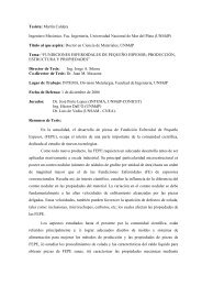
Figure 2.1 B / Cch<br />
ratio as a function of Eb / N 0<br />
(2.5)
Chapter 2: Combined coding and modulation techniques 13<br />
This curve defines two regions, the one of practical systems, which is the upper right<br />
region, and that of non-practical systems, which is the left down region.<br />
The Shannon relationship states a limiting value of the bit energy-to-noise power<br />
spectral density ratio Eb / N0<br />
, known as the Shannon limit.<br />
Defining the parameter;<br />
E<br />
x =<br />
N<br />
b<br />
0<br />
C<br />
ch<br />
B<br />
The following expression can be obtained:<br />
C<br />
B<br />
E C<br />
E<br />
/<br />
ch b ch<br />
1/<br />
x<br />
b<br />
1 x<br />
= log 2 ( 1+<br />
x)<br />
; 1 = log 2 ( 1+<br />
x)<br />
(2.6)<br />
N 0 B<br />
N 0<br />
As seen in Fig. 2.1, if B Cch<br />
→ ∞,<br />
Cch<br />
B → 0 the limit <strong>over</strong> the quantity Eb N 0 is<br />
reached, and it is equal to:<br />
Eb N<br />
0<br />
1<br />
= = 0.<br />
693 ≡ ( −1.<br />
59 dB)<br />
(2.7)<br />
log e<br />
2<br />
which is the Shannon limit. For orthogonal signaling for instance, this limit is reached<br />
when dimensionality tends to infinity.<br />
Hence bounds for a communication system are stated in terms of both bandwidth and<br />
error probability. The Shannon theorems take into account not only the effect of noise<br />
but also this effect in relationship to bandwidth constraints. The Nyquist theorem<br />
states conditions for transmission without ISI.<br />
Transmission of orthogonal signals can be implemented among other ways by using<br />
M-ary Frequency Shift Keying (MFSK). The transmission of orthogonal signals is<br />
shown to approach the Shannon limit when the dimensionality of the signal set is<br />
increased. The application of coding at binary level is shown also to reach error-free<br />
transmission when the length of the codeword tends to infinity, as stated by the second
Chapter 2: Combined coding and modulation techniques 14<br />
Shannon theorem. Therefore by increasing either the complexity of the coding<br />
procedure in coded systems transmitting classic binary signals, or the dimensionality<br />
of the signal set of the transmission in classic modulation techniques, the performance<br />
of the system tends to the Shannon limit, and it is reached when the corresponding<br />
parameter is increased to infinity.<br />
At this point a combined technique that uses coding and modulation as one operation<br />
[43], appears to be a good method to approach that limit without making the involved<br />
parameters tend to infinity. A coding gain is expected from the coding procedure, and<br />
also a gain is expected from the proper design of a good N-dimensional signal set, so<br />
that the addition of these gains reduces the gap to the Shannon limit for a<br />
communication system.<br />
The use of coding implemented as an independent operation is indeed in agreement<br />
with the above idea. The binary format is constructed on a set of baseband signals that<br />
are orthogonal in time. Increasing the codeword length represents an increase of the<br />
dimensionality of the signal set used in this case, whatever the selected format (polar,<br />
bipolar, with or without return to zero format). In this sense the Shannon theorem<br />
states its limit for binary information that has been mapped into a particular signal set,<br />
that is a square shape baseband signal set constructed using orthogonal in-time basis<br />
functions. It can be expected that a selection of a mapping procedure <strong>over</strong> a better<br />
signal set can approach the same performance as the classic binary format with a<br />
lower dimensionality.<br />
One of the most important contributions to the so-called combined coding and<br />
modulation technique has been the work of Ungerboeck [44, 45].<br />
2.3 Trellis-Coded Modulation: A combined coding and modulation technique<br />
2.3.1 <strong>Coding</strong> and modulation<br />
As presented in previous section, the promise of noise-free transmission predicted by<br />
the Shannon theorem can be reached by a proper use of coding. However, the<br />
improvement provided by any coding technique implies a reduction of the
Chapter 2: Combined coding and modulation techniques 15<br />
transmission rate or equivalently, an increase of the transmission bandwidth. On the<br />
other hand it is also possible to provide an improvement in performance of a<br />
communication system by increasing the dimensionality of the signal set used for the<br />
transmission. The use of a combined technique in which coding is thought of as an<br />
operation <strong>over</strong> mathematical identities that represent a given signal of a modulation<br />
scheme will involve the transmission of coded signals providing an improvement in<br />
the performance of a communication system. Thus, the optimisation of both the<br />
properties of the signal set used for the transmission, and the coding technique itself,<br />
should be made taking into account the relationship between these entities, whose<br />
optimisation becomes another aim of the design.<br />
In this sense, TCM [44] has been one of the most important steps in the application of<br />
the idea of combining these two entities. Ungerboeck [45] presented in his paper a<br />
technique in which the transmission of independent symbols is replaced by the<br />
transmission of sequences that are designed directly <strong>over</strong> a constellation of signals of<br />
a modulated scheme which is of a higher order than the initial one, so that the process<br />
of using a constellation with an increased normalised bit rate allows us to cancel the<br />
bit rate penalty produced by the coding procedure. Thus, TCM provides an<br />
improvement <strong>over</strong> the performance of the communication system without increasing<br />
the transmitted power or the required bandwidth.<br />
The demodulation and decoding of this transmission should be made at the same time,<br />
based on soft decision of the transmitted sequence of signals <strong>over</strong> a trellis.<br />
Thus, coding and modulation are applied as a single operation. The apparent reduction<br />
of the minimum distance among signals of the higher order constellation is <strong>over</strong>come<br />
by using the transmission of sequences of dependent signals generated by<br />
convolutional coding, rather than independent signals.<br />
2.3.2 Introduction to the idea of TCM<br />
The design of TCM schemes was initially performed <strong>over</strong> the MPSK constellation<br />
[45, 44, 46, 53, 54, 55, 57, 58, 59] for different channels. If a given system<br />
transmitting one bit in a period of T seconds is found to be inefficient in terms of the
Chapter 2: Combined coding and modulation techniques 16<br />
bit error rate, it should be improved for instance by a proper use of convolutional<br />
coding. If a convolutional code of rate 1/2 is used for example, it will require a twice<br />
of the bandwidth to keep the transmission at the same rate with improved error<br />
probability performance. Transmission of 1 bit in a period T can be made using a<br />
modulation like 2PSK. The time diagram and the corresponding constellation are<br />
shown in Fig. 2.2.<br />
Figure 2.2 2PSK transmission and the corresponding constellation<br />
If as a result of the convolutional coding the source bit ‘1’ in Fig. 2.2 produces for<br />
instance a word of two bits, say ‘1 0’, the corresponding time diagram is that of Fig.<br />
2.3.<br />
+1<br />
+1<br />
-1<br />
T sec<br />
T sec<br />
Figure 2.3 4PSK transmission and the corresponding constellation<br />
2PSK<br />
constellation<br />
4PSK<br />
constellation<br />
The bit in Fig 2.2 is encoded by the sequence of Fig. 2.3, which is transmitted <strong>over</strong> a<br />
higher dimension constellation. As is well known the bandwidth of the 4PSK
Chapter 2: Combined coding and modulation techniques 17<br />
transmission for an information rated as it seen in Fig. 2.3 is the same as the<br />
bandwidth needed for transmitting the signal of Fig. 2.2 using 2PSK. In this way, the<br />
effect of the coding rate is hidden by the use of a higher level constellation. The<br />
coding technique is applied in combined way with modulation without bandwidth<br />
expansion.<br />
In spite of the reduction in the distance among signals of the higher level<br />
constellation, the use of convolutional coding provides transmission of sequences of<br />
dependent signals rather than independent ones. Therefore careful design of the<br />
convolutional coding procedure can provide a given coding gain to the system,<br />
without increasing the bandwidth.<br />
2.3.3 Definition of parameters for TCM<br />
Any signal to be transmitted can be represented as a vector in an N-dimensional<br />
Euclidean <strong>Space</strong> R N , which is often called the signal space. The channel is modelled<br />
as an Additive White Gaussian Noise (AWGN) channel in which the noise affects a<br />
given signal generating an hypersphere around the given signal vector. When a signal<br />
vector s is transmitted the received signal vector can be represented by<br />
r = s + n<br />
(2.8)<br />
where n is a noise vector whose components are independent Gaussian random<br />
variables with zero mean value and variance N / 2 .<br />
The signal set S is composed of M signals (vectors), and the average energy of the<br />
set is given by:<br />
1<br />
E =<br />
M<br />
∑<br />
s∈S<br />
|| s ||<br />
2<br />
0<br />
(2.9)<br />
where || . || is the norm of a vector. A given sequence of signals (vectors) of length K<br />
can be constituted by an orthogonal-in-time composition of signals of the set S . The
Chapter 2: Combined coding and modulation techniques 18<br />
Euclidean distance between any two sequences s b0<br />
, sb1<br />
,..., sbK<br />
−1<br />
, and s a0<br />
, sa1,...,<br />
saK<br />
−1<br />
is<br />
given by the following expression:<br />
∑ − K 1<br />
i=<br />
0<br />
2<br />
2<br />
d = || s − s ||<br />
(2.10)<br />
bi<br />
ai<br />
If a given code C is constituted from a set of sequences, the minimum squared<br />
Euclidean distance between any two sequences will be considered as the minimum<br />
2<br />
squared Euclidean distance d min<br />
2.3.4 Coded and uncoded sequences<br />
of the code C .<br />
When there is no coding procedure <strong>over</strong> the labels that correspond to the signals of the<br />
constellation, the resulting transmitted sequence is composed of independent signals.<br />
In this case a signal can be followed by any other of the constellation, so that the<br />
minimum squared Euclidean distance of the sequence can be calculated by minimising<br />
2<br />
the terms || − s || ; i = 1,<br />
2,...,<br />
K −1<br />
independently. Therefore:<br />
d<br />
s<br />
2<br />
min<br />
b<br />
≠ s<br />
= min||s<br />
a<br />
∀<br />
sbi ai<br />
bi<br />
s<br />
− s<br />
a<br />
,s<br />
b<br />
ai<br />
||<br />
2<br />
The symbol error probability is upper bounded by:<br />
M −1<br />
⎛<br />
≤ ⎜ d<br />
P(<br />
e)<br />
erfc<br />
2 ⎜<br />
⎝ 2.<br />
N<br />
0<br />
⎞<br />
⎟<br />
⎟<br />
⎠<br />
(2.11)<br />
min (2.12)<br />
Two parameters are defined for comparison proposes; the bandwidth efficiency:<br />
log 2 M<br />
R = (2.13)<br />
N
Chapter 2: Combined coding and modulation techniques 19<br />
where N is the dimensionality of the signal set, and the normalised squared minimum<br />
distance or energy efficiency:<br />
2<br />
d min<br />
2<br />
δ = . log 2 M<br />
(2.14)<br />
E<br />
In view of these definitions, the upper bound of the symbol error probability is given<br />
by [44]:<br />
M −1<br />
⎛<br />
≤ ⎜<br />
δ<br />
P erfc<br />
2 ⎜<br />
⎝ 2<br />
where<br />
E b<br />
E<br />
N<br />
b<br />
0<br />
⎞<br />
⎟<br />
⎠<br />
(2.15)<br />
E<br />
= (2.16)<br />
M<br />
log 2<br />
is the average energy per bit. The above expression shows that a given coding gain<br />
can be obtained by increasing the parameter δ .<br />
As expressed above, the aim of the application of TCM is to provide dependent<br />
sequences of signals designed <strong>over</strong> a constellation of at least one level more than the<br />
uncoded one that corresponds to the given transmission rate. Normally, the<br />
constellation is doubled in size (ie., = 2M<br />
).<br />
M e<br />
The selection of the sequences of dependent nature can be done also <strong>over</strong> the same<br />
original signal set S , to provide traditional convolutional coding by reducing the bit<br />
rate, or <strong>over</strong> an expanded set S e of signals so that M e > M . The minimum distance<br />
d free between any two possible dependent sequences of K signals of the expanded set<br />
S e , should be increased with respect to the minimum distance d min between any two<br />
signals of the set S . If maximum likelihood sequence detection is applied, the<br />
technique will provide a distance gain of:
Chapter 2: Combined coding and modulation techniques 20<br />
d<br />
d<br />
2<br />
free<br />
2<br />
min<br />
Thus, the use of TCM is based on:<br />
(2.17)<br />
• The transmission of dependent sequences of symbols that are mapped into an<br />
expanded constellation of signals; and<br />
• The use of proper expanded constellations.<br />
The generation of dependent sequences is based on the fact that the transmitted signal<br />
s n at the discrete time n depends not only on the corresponding symbol n<br />
on a finite number of previous source symbols [44, 46]:<br />
s<br />
n<br />
n<br />
= f ( a , a<br />
σ = ( a<br />
n<br />
n−1<br />
, a<br />
n−1<br />
n−2<br />
,..., a<br />
,..., a<br />
n−L<br />
)<br />
n−L<br />
These expressions can be given briefly as:<br />
s<br />
σ<br />
n<br />
= f ( a , σ )<br />
n<br />
n<br />
= g(<br />
a , σ )<br />
n+<br />
1 n n<br />
a<br />
n<br />
)<br />
Memory σ n<br />
Figure 2.4 Block diagram of a TCM scheme<br />
Select subset from<br />
constellation<br />
<strong>Signal</strong> from subset<br />
s n<br />
a , but also<br />
(2.18)<br />
(2.19)
Chapter 2: Combined coding and modulation techniques 21<br />
2.3.5 An example of TCM<br />
As explained, the design of simple trellis codes is based on the fact of using a<br />
convolutional encoder whose outputs are mapped into an expanded constellation, so<br />
that the effect of the bit rate reduction of the code is hidden by the effect of an<br />
increased rate obtained with the expanded constellation. As will be seen, the coding<br />
gain of a given TCM scheme can be increased by optimising the so-called<br />
constellation gain, the shaping gain, and the coding gain [1, 6, 9, 16]. In the example<br />
below, the total gain is calculated. This total gain is studied in comparison to an<br />
equivalent uncoded system that uses the same <strong>over</strong>all bit rate and bandwidth.<br />
Consider the convolutional encoder of Fig. 2.5.<br />
a 1<br />
a 2<br />
a 3<br />
Figure 2.5 A 1/2-rate convolutional encoder<br />
y 1<br />
y<br />
0<br />
Mapping <strong>over</strong> a<br />
4PSK constellation<br />
00 → +1<br />
01 → +j<br />
10 → -j<br />
11 → -1
Chapter 2: Combined coding and modulation techniques 22<br />
a 1 a 2 a 3 a 1 a 2 y 1 y 0<br />
0 0 0 0 0 0 0 +1<br />
1 0 0 1 0 1 1 -1<br />
0 1 0 0 1 0 1 +j<br />
1 1 0 1 1 1 0 -j<br />
0 0 1 0 0 1 1 -1<br />
1 0 1 1 0 0 0 +1<br />
0 1 1 0 1 1 0 -j<br />
1 1 1 1 1 0 1 +j<br />
Table 2.1 Transitions for the encoder of Fig. 2.5<br />
The trellis for the system is shown in Fig. 2.6:<br />
00<br />
01<br />
10<br />
11<br />
(1,-1)<br />
(0,-1)<br />
(1,+1)<br />
(0,+j)<br />
(1,-j)<br />
(0,-j)<br />
(0,+1)<br />
(1,+j)<br />
Figure 2.6 Trellis for the encoder of Fig. 2.5<br />
And the path of minimum distance from the all-zero sequence is seen in Fig. 2.7:<br />
+ 1 + 1<br />
+<br />
1<br />
− 1<br />
+ j<br />
− 1<br />
Figure 2.7 Path of minimum distance for the trellis of Fig. 2.6
Chapter 2: Combined coding and modulation techniques 23<br />
The distance of this path is calculated:<br />
d<br />
2<br />
free<br />
= 2<br />
2<br />
+ (<br />
2)<br />
2<br />
+ 2<br />
2<br />
= 10<br />
so the coding gain <strong>over</strong> uncoded 2PSK is<br />
⎛ d<br />
⎜<br />
⎜<br />
⎝ d<br />
2<br />
free<br />
10. log ⎟<br />
10 = 10.<br />
log<br />
2<br />
10 ⎟<br />
min<br />
⎞<br />
⎠<br />
⎛10<br />
⎞<br />
⎜ ⎟ = 3.<br />
97dB<br />
⎝ 4 ⎠<br />
2.3.6 Proper selection of the signal set. The set partitioning<br />
As seen in the previous example, the assignment of the signal labels in the<br />
corresponding trellis defines the distance properties of the scheme. The squared<br />
Euclidean free distance is calculated as the cumulated distance between any two<br />
sequences described by the corresponding trellis, which emerge from and return to a<br />
particular state. When parallel transitions exist, the distance is calculated <strong>over</strong> a path<br />
of length L = 1,<br />
as shown in Fig. 2.8.<br />
Figure 2.8 A parallel transition between two states<br />
For two signal sequences a<br />
( b1<br />
b2<br />
bL<br />
S and b<br />
S , composed of signals ) ,..., , s s s and<br />
( a1<br />
a2<br />
aL<br />
s , s ,..., s ) respectively, and when the squared free distance is not determined by<br />
the parallel transitions, calculation of this parameter has to be made <strong>over</strong> paths of<br />
length L .<br />
σ n<br />
s<br />
s<br />
a,<br />
n+<br />
1<br />
b,<br />
n+<br />
1<br />
σ<br />
n+<br />
1
Chapter 2: Combined coding and modulation techniques 24<br />
Figure 2.9 Transition of length L<br />
Therefore the squared Euclidean free distance is calculated <strong>over</strong> all the paths of length<br />
L :<br />
σ n<br />
s<br />
2 2<br />
2<br />
d free = d ( sa,<br />
n+<br />
1,<br />
sb,<br />
n+<br />
1)<br />
+ ... + d ( sa,<br />
n+<br />
L , sb,<br />
n+<br />
L )<br />
(2.20)<br />
2<br />
where d ( sai<br />
, sbi<br />
) denotes the squared distance between signals ai<br />
s and bi<br />
Maximisation of the squared Euclidean free distance of the TCM scheme is obtained<br />
by applying a procedure suggested by Ungerboeck [45], and called set partitioning. In<br />
a set partitioning, all the signals of each subset have the same value of the squared<br />
distance, and the squared distance for a given subset increases in the next step of the<br />
partition procedure.<br />
sa, n+<br />
1<br />
a,<br />
n L<br />
b,<br />
n+<br />
1<br />
σ n+<br />
1<br />
. . .<br />
σ n+L<br />
−1<br />
A classic example is shown in the Fig. 2.10. It is applied to the 8PSK constellation.<br />
The values of the minimum squared distance in each subset are calculated on a basis<br />
of a radius of the constellation equal to 1.<br />
s +<br />
s b,<br />
n+<br />
L<br />
σ n+ L<br />
s .
Chapter 2: Combined coding and modulation techniques 25<br />
4<br />
Figure 2.10 Set partitioning for an 8PSK constellation<br />
The partition method also can be applied to a set of 8 signals that geometrically form a<br />
cube:<br />
5<br />
4<br />
0<br />
2<br />
5<br />
6<br />
1<br />
Figure 2.11 Set partitioning for a cube<br />
0<br />
2<br />
6<br />
4<br />
3<br />
5<br />
0<br />
2<br />
6<br />
5<br />
4<br />
0 1<br />
1<br />
7<br />
5<br />
6<br />
4<br />
0<br />
6<br />
3<br />
3<br />
1<br />
2<br />
d min =<br />
0.<br />
58<br />
2<br />
4<br />
0 1<br />
7<br />
1<br />
5 7<br />
3<br />
6<br />
2<br />
2<br />
d min =<br />
3<br />
7<br />
2<br />
2<br />
d min =<br />
7<br />
2<br />
3<br />
4<br />
7
Chapter 2: Combined coding and modulation techniques 26<br />
2.4 Representations and design for TCM<br />
2.4.1 Introduction<br />
There are basically two representations for a TCM encoder. The Ungerboeck<br />
representation [45] is based on the use of a convolutional encoder that represents the<br />
memory of the system, and also of a selector for the partition of the set of signals. The<br />
Calderbank-Mazo representation [47] shows an analytical expression for the mapping<br />
between source symbols and signals of the constellation.<br />
2.4.2 The Ungerboeck representation<br />
In a TCM encoder-modulator a source symbol a i corresponding to the time instant i<br />
can be assigned to one of<br />
k<br />
2 values, represented as sequences of k binary digits<br />
( 1)<br />
( 2)<br />
( k )<br />
b i , bi<br />
,..., bi<br />
. The encoder output c i at the time instant i depends on the input,<br />
represented by the binary digits, and on previous ν ≥ 0 bits , j = 1,<br />
2,...,<br />
k :<br />
( 1)<br />
( 1)<br />
( 1)<br />
( k ) ( k ) ( k )<br />
c = f ( bi<br />
, bi−1<br />
,..., b − ,..., bi<br />
, bi−1<br />
,..., b − )<br />
(2.21)<br />
i i v1<br />
i vk<br />
The encoder presents two parts. One is the memory, implemented by using a binary<br />
convolutional encoder with k binary inputs<br />
( 1)<br />
i<br />
( 2)<br />
i<br />
( n)<br />
i<br />
j<br />
( 1)<br />
i<br />
( 2)<br />
i<br />
( k )<br />
i<br />
b , b ,..., b and n binary outputs<br />
c , c ,..., c . The other is the memoryless part, which is basically a modulator that<br />
maps the binary n-tuple output into a signal s i of the constellation.
Chapter 2: Combined coding and modulation techniques 27<br />
(k<br />
b i<br />
b<br />
Figure 2.12 Ungerboeck representation of a TCM scheme<br />
2.4.3 The Analytic Description. Calderbank-Mazo representation<br />
Calderbank and Mazo described the TCM encoder as a generator of channel signals<br />
that depend on m data bits ( a a ,..., a )<br />
( a ,..., a )<br />
1 , 2 m and on ν previous input bits<br />
m+<br />
1 , m+<br />
2 m v . The output signal s is a function of ν<br />
a +<br />
)<br />
( k −1)<br />
i<br />
b<br />
( 1)<br />
i<br />
Convolutional encoder<br />
with constraint length<br />
v =<br />
k<br />
∑ vi<br />
i=<br />
1<br />
n = m + binary input bits,<br />
called the sliding block of input bits. The block diagram is presented in Fig. 2.13:<br />
a m<br />
a<br />
m~<br />
+ 1<br />
a m~<br />
a 1<br />
.<br />
.<br />
.<br />
.<br />
.<br />
.<br />
b<br />
b<br />
m<br />
m~<br />
+ 1<br />
b~ m<br />
b 1<br />
.<br />
.<br />
.<br />
(n<br />
c i<br />
Fig 2.13 Block diagram of the Analytic Description [47]<br />
.<br />
.<br />
.<br />
Memory<br />
c<br />
)<br />
( n−1)<br />
i<br />
c<br />
( 1)<br />
i<br />
b<br />
b m<br />
m~<br />
+ 1<br />
b~ m<br />
b 1<br />
b m+<br />
v<br />
.<br />
.<br />
.<br />
b m+<br />
1<br />
Mapping of<br />
binary n-tuples<br />
into signals si of<br />
the constellation<br />
s i<br />
, ,..., ) b b b c s<br />
( 1 2 n
Chapter 2: Combined coding and modulation techniques 28<br />
The parameter b~ m identifies a variable m ~ that defines the number of input bits related<br />
with the memory part of the scheme. The output function has as argument the binary<br />
n-tuple ( a a ,..., a )<br />
1 , 2<br />
n<br />
m<br />
:<br />
n<br />
c(<br />
a , a ,..., a ) = c + ∑c<br />
a + ∑ c a a + ... + ∑ c<br />
1<br />
2<br />
0<br />
=<br />
i<br />
i 1<br />
i<br />
> =<br />
j i<br />
j i<br />
ij<br />
, 1<br />
i<br />
j<br />
> ><br />
=<br />
ijl<br />
i,<br />
j,<br />
l 1<br />
l j i<br />
a a a + ... + c<br />
i<br />
j<br />
l<br />
12...<br />
n 1<br />
a a ... a<br />
2<br />
n<br />
(2.22)<br />
The Analytic Description is more conveniently used when coefficients are of the form<br />
of ± 1. Therefore a conversion as shown in Fig. 2.13 is done by using the following<br />
expression:<br />
bi = 1−<br />
2ai<br />
i = 1,<br />
2,...,<br />
n<br />
(2.23)<br />
The expression of the output as a function of the input vector is now of the form:<br />
n<br />
n<br />
c(<br />
b , b ,..., b ) = d + ∑ d b + ∑ d b b + ... + ∑ d<br />
1<br />
2<br />
0<br />
i=<br />
1<br />
i<br />
i<br />
i,<br />
j=<br />
1<br />
j><br />
i<br />
ij<br />
i<br />
j<br />
i,<br />
j,<br />
l=<br />
1<br />
l><br />
j><br />
i<br />
This equation can be expressed in matrix form as:<br />
l<br />
l<br />
c<br />
ijl<br />
b b b + ... + d<br />
i<br />
j<br />
l<br />
12...<br />
n 1<br />
b b ... b<br />
2<br />
n<br />
(2.24)<br />
C = B D<br />
(2.25)<br />
where<br />
⎡ c(<br />
1,<br />
1,...,<br />
1)<br />
⎤<br />
⎢ ⎥<br />
⎢<br />
c(<br />
-1,<br />
1,...,<br />
1)<br />
⎥<br />
⎢ . ⎥<br />
= ⎢ ⎥<br />
⎢ . ⎥<br />
⎢ . ⎥<br />
⎢ ⎥<br />
⎢⎣<br />
c(<br />
-1,<br />
-1,...,<br />
-1)<br />
⎥⎦<br />
C l (2.26)
Chapter 2: Combined coding and modulation techniques 29<br />
i<br />
[ b b . . . b , b b , b b , b b , . . . b b b ]<br />
B = ... (2.27)<br />
1 1 2<br />
n 1 2 2 3 1 3<br />
1 2<br />
[ d , d , . . . d ]<br />
T<br />
D c = 0 1<br />
12...<br />
n<br />
(2.28)<br />
B i is the i-th row of B l , and it is composed of coefficients b i that are taken from the<br />
argument of the i-th row of l C . For D-dimensional modulation C l and D c are of a<br />
n<br />
size 2 xD , and B l is always<br />
n n<br />
2 x2 .<br />
Here n = k + ν . Calderbank and Mazo have shown that Bl is an orthogonal matrix.<br />
Equation (2.25) is solved by:<br />
D<br />
c<br />
T<br />
l Cl<br />
n<br />
B<br />
= (2.29)<br />
2<br />
Based on the Analytic Description the design procedure applies design rules proposed<br />
by Ungerboeck [45] and Turgeon [44], to finally describe the TCM encoder in the<br />
more convenient form of Ungerboeck, after transforming it from the Calderbank-<br />
Mazo representation. The Ungerboeck representation to be used in the design<br />
procedure is shown below:<br />
am<br />
a<br />
m~<br />
+ 1<br />
a m~<br />
a1<br />
.<br />
.<br />
.<br />
.<br />
.<br />
.<br />
Convolutional<br />
Encoder of rate<br />
m ~<br />
m~<br />
+ 1<br />
Figure 2.14 Block diagram of an Ungerboeck representation of a TCM scheme<br />
ym<br />
y m+1<br />
y m~<br />
y0<br />
The convolutional encoder provides<br />
m+1 output bits<br />
.<br />
.<br />
.<br />
.<br />
.<br />
.<br />
n<br />
2 m+1 signals of<br />
the constellation<br />
s
Chapter 2: Combined coding and modulation techniques 30<br />
2.4.4 Ungerboeck and Turgeon rules<br />
The design procedure based on expression (2.29) applies rules stated by Ungerboeck<br />
and Turgeon, for the signal assignment to trellis transitions.<br />
A description of minimal complexity is one with the minimum number of<br />
d coefficients so that each bit of the input sliding block appears only once in the<br />
encoder formula.<br />
Ungerboeck rules for assigning signals of the constellation to a given transition in the<br />
corresponding trellis are [44, 45]:<br />
• All signals of the constellation appear the same number of times in the assignment,<br />
making the code be composed of equiprobable signals.<br />
• When the trellis that defines the TCM encoder has parallel transitions, signals<br />
corresponding to the same subset of highest intrasubset distance should be assigned<br />
to those parallel transitions.<br />
• The m<br />
2 transitions that emerge from or return to a given state should be assigned<br />
signals from one subset at the first level of the partitioning.<br />
The Maximum <strong>Signal</strong> Value (MSV) is the maximum numerical value of a signal.<br />
When the signal has a vectorial expression, the MSV is the maximum sum of the<br />
vector co-ordinates.<br />
A signal difference represents the difference between any two signals when only one<br />
bit of the input sliding block is changed. The absolute signal difference is the absolute<br />
value of the signal difference. Thus, the signal difference is given by the following<br />
expression:<br />
δ = x b , b ,..., b ,..., b , b + ,..., b ) − x(<br />
b , b ,..., −b<br />
,..., b , b + ,..., b ) (2.30)<br />
i<br />
( 1 2 i k k 1 n 1 2 i k k 1 n<br />
Turgeon rules are useful for minimising the encoder formula:
Chapter 2: Combined coding and modulation techniques 31<br />
• State 1 is assigned a sequence of signals that starts at level m of the set partitioning,<br />
so that signals of the two-signal subset containing the MSV are the first to be<br />
established for that state. Then the procedure is repeated for one level up from the<br />
previous one of the set partitioning. The process is repeated until finishing the<br />
definition of the first state.<br />
• Each input bit should be associated with a unique signal difference.<br />
The conversion of the Analytic representation to the Ungerboeck representation is<br />
done using Turgeon’s procedure [44]. Output bits z 0 , z1,...,<br />
zm<br />
are mapped into the<br />
signal constellation so that a mapping rule should be determined. Then the output<br />
signal s has to be expressed as a function of the output bits z i . This can be done by<br />
finding for ; i = 1,<br />
2,...,<br />
m , the signal difference in each dimension between z = −1<br />
z i<br />
and z i = 1.<br />
z i is then assigned to a coefficient half their corresponding signal<br />
difference.<br />
After relating each dimension of the signal s to the input bits n b b b ,..., , 0 1 , and the<br />
output bits z 0 , z1,...,<br />
zm<br />
, the output bits can be related to the input bits. Finally, this<br />
last relationship provides the structure of the convolutional encoder. The<br />
conventional binary form with 0 and 1 as binary values is obtained by taking into<br />
account that a multiplication in the ± 1 convention is equivalent to a XOR operation in<br />
the 0 and 1 convention. In this way, bits y 0 , y1,...,<br />
ym<br />
are at the end related to bits<br />
a a ,..., a corresponding to the Ungerboeck description of Fig. 2.14.<br />
0 , 1<br />
n<br />
2.4.5 Examples of the design procedure<br />
The system of the example given in section 2.3.5 will be now designed using the<br />
above procedure. This system is a TCM scheme that uses the 4PSK constellation as an<br />
expanded set of signals, to transmit 1 bit during the transmission period. The<br />
associated trellis is of rate 1/2, and it has 4 states, with two branches emerging and re-<br />
merging from each state. There are no parallel transitions.<br />
i
Chapter 2: Combined coding and modulation techniques 32<br />
The input bit relationship for the 1/2 rate, four-state trellis, is shown in Fig. 2.15:<br />
Figure 2.15 Input bit structure of a 1/2 rate convolutional code<br />
The constellation to be used is a 4PSK constellation, labeled as shown in Fig. 2.16:<br />
Figure 2.16 Labels for a 4PSK constellation<br />
and as is well known, the set partitioning for this constellation is that seen in Fig.<br />
2.17:<br />
-3<br />
2<br />
b 1 b 2<br />
3<br />
T T<br />
b<br />
1<br />
1<br />
3<br />
-1<br />
2<br />
2 0<br />
Figure 2.17 A set partitioning for a 4PSK constellation<br />
1<br />
3<br />
0<br />
0<br />
3<br />
1<br />
3
Chapter 2: Combined coding and modulation techniques 33<br />
The table of the signal mapping is the following:<br />
z 1 1 1 -1 -1<br />
z 0 1 -1 -1 1<br />
s [3] [1] [-3] [-1]<br />
Table 2.2 <strong>Signal</strong> mapping<br />
Then the signal s is obtained as:<br />
s = 2z1 + z0<br />
Equation (2.25) applied to this particular example results in the following set of<br />
equations:<br />
c<br />
c<br />
c<br />
c<br />
c<br />
c<br />
c<br />
c<br />
( 1,<br />
1,<br />
1)<br />
= + 3 = d1<br />
+ d 2 + d3<br />
+ d12<br />
+ d13<br />
+ d 23 + d123<br />
( −1,<br />
1,<br />
1)<br />
= −3<br />
= −d1<br />
+ d 2 + d3<br />
− d12<br />
− d13<br />
+ d 23 − d123<br />
( 1,<br />
−1,<br />
1)<br />
= + 1=<br />
d1<br />
− d 2 + d3<br />
− d12<br />
+ d13<br />
− d 23 − d123<br />
( −1,<br />
−1,<br />
1)<br />
= −1=<br />
−d1<br />
− d 2 + d 3 + d12<br />
− d13<br />
− d 23 + d123<br />
( 1,<br />
1,<br />
−1)<br />
= −3<br />
= d1<br />
+ d 2 − d 3 + d12<br />
− d13<br />
− d 23 − d123<br />
( −1,<br />
1,<br />
−1)<br />
= + 3 = −d1<br />
+ d 2 − d 3 − d12<br />
+ d13<br />
− d 23 + d123<br />
( 1,<br />
−1,<br />
−1)<br />
= −1=<br />
d1<br />
− d 2 − d3<br />
− d12<br />
− d13<br />
+ d 23 + d123<br />
( −1,<br />
−1,<br />
−1)<br />
= + 1=<br />
−d1<br />
− d 2 − d3<br />
+ d12<br />
+ d13<br />
+ d 23 − d123<br />
The solution for this equation system is d = , d = 1,<br />
and the rest of the coefficients<br />
are zero.<br />
13<br />
2 123<br />
Thus, the signal output is given as a function of bits bi as:<br />
s =<br />
2b b + b b b<br />
1<br />
3<br />
1<br />
2<br />
3
Chapter 2: Combined coding and modulation techniques 34<br />
Then, the implementation of the encoder in the Analytic Description form is shown in<br />
Fig. 2.18:<br />
Figure 2.18 A convolutional encoder for example of section 2.3.5<br />
The relationship between the signal s and the input bits, and this signal and the output<br />
bits, allows us to obtain the relationship between input and output bits:<br />
z<br />
z<br />
1<br />
0<br />
= b b<br />
1<br />
1<br />
3<br />
= b b b<br />
2<br />
3<br />
The corresponding relationship with the input bits in 1 and 0 representation leads to<br />
the following expressions:<br />
y<br />
y<br />
1<br />
0<br />
= a ⊕ a<br />
1<br />
1<br />
3<br />
= a ⊕ a ⊕ a<br />
2<br />
3<br />
Thus, the resulting convolutional encoder is that shown in Fig. 2.5. In this particular<br />
case the topology is not minimal, in the sense that inputs a 1 and a 3 appears twice in<br />
the final formula. If another design <strong>over</strong> a similar scheme is essayed, a labelling of the<br />
constellation is varied as shown in Fig. 2.19, where a natural assignment of bits is<br />
done:<br />
b1 2<br />
T<br />
b2 T<br />
b3 +<br />
+
Chapter 2: Combined coding and modulation techniques 35<br />
-1<br />
Figure 2.19 Natural binary mapping for a 4PSK constellation<br />
z 1 1 1 -1 -1<br />
z 0 1 -1 -1 1<br />
s [3] [1] [-3] [-1]<br />
Table 2.3 Natural binary mapping<br />
Then the signal s is obtained as:<br />
s = 2z + z<br />
1<br />
10<br />
0<br />
Now the equation system is expressed as follows:<br />
1<br />
01<br />
11<br />
-3<br />
00<br />
y1y0<br />
3
Chapter 2: Combined coding and modulation techniques 36<br />
c<br />
c<br />
c<br />
c<br />
c<br />
c<br />
c<br />
c<br />
( 1,<br />
1,<br />
1)<br />
= + 3 = d1<br />
+ d 2 + d3<br />
+ d12<br />
+ d13<br />
+ d 23 + d123<br />
( −1,<br />
1,<br />
1)<br />
= −1=<br />
−d1<br />
+ d 2 + d3<br />
− d12<br />
− d13<br />
+ d 23 − d123<br />
( 1,<br />
−1,<br />
1)<br />
= + 1=<br />
d1<br />
− d 2 + d3<br />
− d12<br />
+ d13<br />
− d 23 − d123<br />
( −1,<br />
−1,<br />
1)<br />
= −3<br />
= −d1<br />
− d 2 + d 3 + d12<br />
− d13<br />
− d 23 + d123<br />
( 1,<br />
1,<br />
−1)<br />
= −1=<br />
d1<br />
+ d 2 − d3<br />
+ d12<br />
− d13<br />
− d 23 − d123<br />
( −1,<br />
1,<br />
−1)<br />
= + 3 = −d1<br />
+ d 2 − d 3 − d12<br />
+ d13<br />
− d 23 + d123<br />
( 1,<br />
−1,<br />
−1)<br />
= −3<br />
= d1<br />
− d 2 − d3<br />
− d12<br />
− d13<br />
+ d 23 + d123<br />
( −1,<br />
−1,<br />
−1)<br />
= + 1=<br />
−d1<br />
− d 2 − d3<br />
+ d12<br />
+ d13<br />
+ d 23 − d123<br />
whose solution is given if d = , d = 2 , and the remaining coefficients are zero. As a<br />
2<br />
1 13<br />
result of this solution, signal s can be obtained as a function of coefficients b i as:<br />
s = 2b b + b<br />
1<br />
3<br />
2<br />
Comparing with the above expression that relates the output bits to the signal s :<br />
z<br />
z<br />
1<br />
0<br />
= b b<br />
1<br />
= b<br />
2<br />
3<br />
The corresponding relationship with the input bits in 1 and 0 representation leads to<br />
the following expressions:<br />
y<br />
y<br />
1<br />
0<br />
= a ⊕ a<br />
1<br />
= a<br />
2<br />
3<br />
The convolutional encoder is shown in Fig. 2.20:
Chapter 2: Combined coding and modulation techniques 37<br />
Figure 2.20 Convolutional encoder for the mapping of Fig. 2.19<br />
The trellis for the system is shown in Fig. 2.21:<br />
00<br />
10<br />
01<br />
11<br />
a 1 a 2<br />
Figure 2.21 Trellis for the convolutional encoder of Fig. 2.20<br />
and the path of minimum distance from the all zero sequence has a squared Euclidean<br />
2 free distance d = 10 .<br />
free<br />
(1,[-1])<br />
(0,[1])<br />
(1,[-3])<br />
(0,[-1])<br />
(1,[3])<br />
(0,[-3])<br />
(0,[3])<br />
(1,[1])<br />
a 3<br />
y 1<br />
y<br />
0<br />
Mapping <strong>over</strong> a<br />
4PSK constellation<br />
00 → [3]<br />
01 → [1]<br />
10 → [-1]<br />
11 → [-3]
Chapter 2: Combined coding and modulation techniques 38<br />
2.5 Performance of TCM<br />
2.5.1 Introduction<br />
By considering TCM as a convolutional coding technique directly mapped into a set<br />
of signals, the performance of TCM is analysed as is made for convolutional coding<br />
but taking into account the metric of the signal set. The calculation of distance<br />
properties should be made <strong>over</strong> the signals of the constellation, and the error events<br />
are also related to that metric.<br />
The main parameter for evaluating a given digital communication system is the error<br />
probability. For TCM schemes the error probability is upper and lower bounded by a<br />
monotonically decreasing function of the increase of the squared Euclidean free<br />
distance<br />
2<br />
d free of the TCM scheme [44].<br />
The squared Euclidean free distance is the main parameter for characterising TCM<br />
schemes <strong>over</strong> the AWGN channel. A TCM scheme attempts a compensation of the<br />
coding rate penalty while providing some additional coding gain by increasing the<br />
squared Euclidean free distance in comparison to the minimum distance of the<br />
uncoded system. A linear measure of this effect is the so-called Asymptotic <strong>Coding</strong><br />
Gain (ACG).<br />
2.5.2 Analysis of the error probability. The error state diagram<br />
A good treatment of performance of TCM schemes is done in [44]. A brief summarize<br />
of related concepts is presented in this section.<br />
Ungerboeck codes are characterised by an input word of m bits that generates an<br />
output of m + 1 binary symbols i<br />
c , mapped into signals s = f c ) , where f (.) defines<br />
the mapping rule. There is a one-to-one correspondence between i s and c i , that are<br />
called the labels of s i an error event of length L is modelled as two label sequences<br />
[44, 48]:<br />
i<br />
( i
Chapter 2: Combined coding and modulation techniques 39<br />
' ' '<br />
c k , ck<br />
+ 1,..., ck<br />
+ L−1<br />
and c k , ck<br />
+ 1,...,<br />
ck<br />
+ L−1<br />
(2.31)<br />
where<br />
c<br />
c<br />
'<br />
k<br />
'<br />
k+<br />
1<br />
...<br />
c<br />
= c<br />
k+<br />
L−1<br />
k<br />
= c<br />
⊕ e<br />
k+<br />
1<br />
= c<br />
k<br />
⊕ e<br />
k+<br />
L−1<br />
k+<br />
1<br />
⊕ e<br />
k + L−1<br />
Two sequences of signals of length L , S L and<br />
valid sequence<br />
(2.32)<br />
'<br />
S L represent an error event when the<br />
'<br />
S L is selected instead of S L . The error probability is evaluated <strong>over</strong> all<br />
possible error events of length L as [44, 48]:<br />
∞<br />
'<br />
P ≤ ∑ ∑ ∑ P[<br />
S ] P[<br />
S → S ]<br />
(2.33)<br />
'<br />
L=<br />
1 SL<br />
SL<br />
≠S<br />
L<br />
L<br />
L<br />
'<br />
where P[ S → S ] is the probability of that the sequence<br />
L<br />
L<br />
being S L the transmitted sequence.<br />
L<br />
'<br />
S L is selected instead of S L ,<br />
Bounds on performance of TCM schemes are found based on the above expression.<br />
Details of the derivation of a bound for the error probability are given in reference<br />
[44], and they lead to the following expression:<br />
P ≤ T ( D)<br />
(2.34)<br />
where<br />
1<br />
−<br />
4 N<br />
D=<br />
e 0<br />
1 T<br />
T ( D)<br />
= 1 G.<br />
1<br />
(2.35)<br />
N<br />
and<br />
∞<br />
∑<br />
L<br />
L=<br />
1 El<br />
≠ 0 n=<br />
1<br />
G = ∑ ∏G(<br />
e )<br />
(2.36)<br />
n
Chapter 2: Combined coding and modulation techniques 40<br />
1 is the all-one N-vector so that 1 G.<br />
1<br />
T<br />
is the sum of all the entries of G .<br />
The signal set defines the values of the entries of the matrices [ e ) ]<br />
selection of the signal set modifies the error probability performance.<br />
2.5.3 Matrix representation of convolutional codes<br />
( i<br />
G , therefore the<br />
As usually defined for block coding, the generator matrix of a given code is related to<br />
the existence of the parity check matrix. Analogously a matrix representation can be<br />
defined for convolutional codes.<br />
( i)<br />
In general terms if m ( D)<br />
sequence then the generator polynomial<br />
( j)<br />
is the i-th input sequence and c ( D)<br />
is the j-th output<br />
( j)<br />
g i can be considered as the encoder transfer<br />
function that relates input i to output j . Then the transfer function matrix G(D) can<br />
be expressed as:<br />
⎡g<br />
⎢<br />
⎢g<br />
G(<br />
D)<br />
=<br />
⎢<br />
⎢<br />
⎢⎣<br />
g<br />
Then:<br />
( 1)<br />
1<br />
( 1)<br />
2<br />
( 1)<br />
k<br />
( D)<br />
( D)<br />
M<br />
( D)<br />
g<br />
g<br />
g<br />
( 2)<br />
1<br />
( 2)<br />
2<br />
( 2)<br />
k<br />
( D)<br />
( D)<br />
M<br />
( D)<br />
...<br />
...<br />
M<br />
...<br />
g<br />
g<br />
g<br />
( n<br />
1<br />
( n<br />
2<br />
( n<br />
k<br />
( 1)<br />
( 2)<br />
( k )<br />
[ m ( D),<br />
m ( D),...,<br />
m ( D)<br />
]<br />
)<br />
( D)<br />
⎤<br />
) ⎥<br />
( D)<br />
⎥<br />
M ⎥<br />
⎥ )<br />
( D)<br />
⎥⎦<br />
(2.37)<br />
m(<br />
D)<br />
= (2.38)<br />
and<br />
( 1)<br />
( 2)<br />
( n)<br />
[ c ( D),<br />
c ( D),...,<br />
c ( D)<br />
]<br />
c(<br />
D)<br />
= (2.39)<br />
So that<br />
c ( D)<br />
= m(<br />
D).<br />
G(<br />
D)<br />
(2.40)
Chapter 2: Combined coding and modulation techniques 41<br />
After multiplexing the output sequences the code word becomes:<br />
( 1)<br />
n ( 2)<br />
n<br />
n−1<br />
( n)<br />
n<br />
c(<br />
D)<br />
= c ( D ) + Dc ( D ) + ... + D c ( D )<br />
(2.41)<br />
2.5.4 Code and error state diagrams for convolutional codes<br />
Finite State Sequence Machines of any kind can be analysed by depicting the so-called<br />
code state diagram. The error state diagram is a modification of the code state diagram<br />
that is intended as a graphic representation of error events for a given finite state<br />
sequence machine. Details of the use of these diagrams are c<strong>over</strong>ed in references [19,<br />
20, 27, 44, 49].<br />
From the error state diagram it is possible to determine the path that emerges from a<br />
state and re-merges to that state of the minimum distance. On the other hand, a<br />
transfer function can be defined <strong>over</strong> the error state diagram for evaluating the<br />
performance of TCM schemes and convolutional coding.<br />
It is shown that the bit error probability for a binary convolutional code decoded using<br />
hard-decision is upper bounded by [49]:<br />
dT ( D,<br />
I )<br />
P b ≤ (2.42)<br />
I = 1,<br />
D=<br />
2 p(<br />
1−<br />
p)<br />
, L=<br />
1<br />
dI<br />
Where p is the probability of channel symbol error, and T ( D,<br />
I ) is the transfer<br />
function for the error state diagram, which is defined in terms of the unit delay<br />
operator D and the indeterminate I , whose exponent is the number of erroneous input<br />
bits for a given transition.<br />
2.5.5 Catastrophic convolutional codes<br />
A catastrophic error is produced when a finite number of errors generates an infinite<br />
number of decoded data bits. Massey and Sain [50] stated the conditions for<br />
convolutional codes of catastrophic behaviour. These conditions are sufficient to
Chapter 2: Combined coding and modulation techniques 42<br />
prove the catastrophic error propagation, and it deals with the matrix representation of<br />
convolutional codes.<br />
The condition for a convolutional code to be non-catastrophic is that it should have an<br />
inverse. A first important conclusion of this fact is that any systematic convolutional<br />
code is non-catastrophic. A particular characteristic of a catastrophic convolutional<br />
code is that there is a closed loop of distance zero to the all-zero sequence in a state<br />
different from the all-zero state. In the corresponding trellis the evaluation of the<br />
minimum squared Euclidean free distance involves infinite sequences of the same<br />
distance. It is quite usual to find that the number of neighbours of the same distance<br />
N free becomes infinite.<br />
2.5.6 Properties of the matrix G<br />
In the error state diagram of a TCM scheme the labels of the branches are the elements<br />
of the matrix G that are related to the Euclidean distance between any two symbols<br />
rather than being related with a metric based on Hamming distance. Therefore the<br />
matrix G , equation (2.36), is related to the Euclidean metric. Any entry of this matrix<br />
states an upper bound on the error probability of an event that occurs as a transition<br />
form state p to state q .<br />
For a given square matrix A , if 1 is an eigenvector of the transpose<br />
it is true that<br />
T<br />
A of that matrix,<br />
T T<br />
1 A = α 1 , where α is a constant, and then the matrix A is called<br />
column-uniform because the sum of its elements in a column is independent of the<br />
column order. The matrix A is row-uniform if A . 1 = β.<br />
1,<br />
where β is constant.<br />
It is shown in [44] that if all the matrices G (e)<br />
are either row-uniform or column-<br />
uniform, the transfer function can be evaluated by using scalar labels for the branches<br />
of the error state diagram. These labels are the sum of the elements of a row or<br />
column. This is related to the degree of symmetry of the constellation of the TCM<br />
scheme, which is considered in these cases as a uniform TCM scheme. G (e)<br />
is row-<br />
uniform if the transitions emerging from a given node of the trellis are associated with<br />
the same set of labels. It is column-uniform if this happens to the transitions ending at<br />
a given node. Here, uniformity of the TCM scheme implies either, that G is row-
Chapter 2: Combined coding and modulation techniques 43<br />
uniform (transitions leaving from any node carry the same set of labels) or column-<br />
uniform (transitions leading to any node carry the same set of labels).<br />
2.5.7 Uniformity<br />
Biglieri et al. [44, 48] state conditions for uniformity. They define the Uniform<br />
Distance Property (UDP) and the Uniform Error Property (UEP), which are given<br />
when the code is said to be uniform. In the definition of uniformity, both the<br />
partitioning set and the labeling procedure are important to keep this condition. These<br />
definitions are particular applications to the concepts of geometrically uniform (GU)<br />
codes defined by Forney [1], for Ungerboeck type TCM schemes.<br />
A lemma stated in [51] considers that C 0 is the set of m<br />
2 vectors c corresponding to<br />
the all-zero state, and forms a commutative group. Then every state in the trellis has<br />
either 0<br />
C or the coset C c~<br />
0 + associated with it.<br />
Then, there are two types of states, those that generates outputs c taken from C0 and<br />
those that generates outputs taken from C c~<br />
0 + . Each row of the matrices<br />
G(e) corresponds either to C 0 or to C c~<br />
0 + .<br />
Therefore all the rows of the error matrices will have equal sum if:<br />
2<br />
2<br />
|| f ( c)<br />
− f ( c⊕e)<br />
||<br />
|| f ( c⊕c<br />
) − f ( c⊕c<br />
⊕e)<br />
||<br />
∑ D = ∑ D<br />
(2.43)<br />
c∈C0<br />
c∈C0<br />
~<br />
~<br />
for any e . This is a sufficient condition for scalar labels. Another way to express this<br />
condition is by considering the mapping between the signal Set S = f ( c),<br />
c ∈ C } and<br />
the labels c , also given by the one-to-one correspondence:<br />
0<br />
{ 0<br />
f ( c)<br />
→ f ( c ⊕ c~<br />
), c ∈ C<br />
(2.44)<br />
where c is considered as all the elements of C 0 . A sufficient condition for uniformity<br />
is that the correspondence of equation (2.44) has to be an isometry, that is, a one-to-<br />
one correspondence, also called a bijection, which preserves scalar products and
Chapter 2: Combined coding and modulation techniques 44<br />
distance properties. Thus, the distance between f (c)<br />
and f ( c ⊕ e)<br />
is the same as the<br />
distance between )<br />
~<br />
f ( c ⊕ c and f ( c ⊕ c<br />
~<br />
⊕ e)<br />
.<br />
When uniformity is given, the branches of the error state diagram are scalars. In this<br />
case the weight profile W (e)<br />
[44] is defined as the value of the sum of elements of<br />
each row of G (e)<br />
:<br />
1<br />
2<br />
|| f ( c)<br />
− f ( c⊕e)<br />
||<br />
W ( e)<br />
= ∑ D<br />
(2.45)<br />
M c∈C<br />
0<br />
These sums are used as labels in the error state diagram. Therefore the transfer<br />
function is:<br />
T ( D)<br />
∑W<br />
( e)<br />
(2.46)<br />
= e<br />
2.5.8 Number of neighbours at the same distance<br />
The following expression:<br />
1 1<br />
ν pq ( dl ) = n1<br />
+ n2<br />
+ ...<br />
(2.47)<br />
L1<br />
L2<br />
M M<br />
takes into account the average number of error paths ni ; i = 1,<br />
2,....<br />
of transitions that<br />
emerge from state p and re-merge to state q after L i time instants that have the same<br />
distance d l as a given path that emerges from state p and re-merges to state q .<br />
then:<br />
1<br />
N(<br />
dl<br />
) = ∑ν<br />
pq ( dl<br />
)<br />
(2.48)<br />
N p,<br />
q<br />
is the average number of competing paths at distance d l associated with a path in the<br />
code trellis of the same distance.
Chapter 2: Combined coding and modulation techniques 45<br />
When l d free<br />
d = , then the number is N = N d ) .<br />
free<br />
( free<br />
Each entry of the matrix G is a power series in the indeterminate D with terms of the<br />
2<br />
l<br />
general form of ( )<br />
d<br />
ν d D . Thus for high signal-to-noise ratios the more significant<br />
pq<br />
l<br />
free<br />
term of this matrix is of the form ν ( d ) D , so that asymptotically the error<br />
probability is<br />
N(<br />
d<br />
free<br />
) e<br />
2<br />
−d<br />
free<br />
N0<br />
.<br />
2.6 Upper bounds for error probability and bit error probability [44, 59]<br />
2.6.1 Upper bounds<br />
pq<br />
A better approximation for an upper bound on P is obtained by calculating exactly<br />
the term that has been bounded by the Bhattacharyya bound. Then<br />
P[<br />
C<br />
where<br />
⎛ ' ⎞<br />
' 1 ⎜ || f ( CL<br />
) − f ( CL<br />
) ||<br />
→ C ] =<br />
⎟<br />
L erfc<br />
2 ⎜<br />
⎟<br />
⎝ 2 N 0 ⎠<br />
L (2.49)<br />
2<br />
erfc(<br />
k)<br />
= ∫ e<br />
π x<br />
∞ 2<br />
−λ<br />
and the inequality<br />
λ + µ<br />
erfc ≤ erfc<br />
2<br />
dλ<br />
= 2Q<br />
λ<br />
e<br />
2<br />
µ / 2<br />
( 2.<br />
k )<br />
provides a bound on error probability:<br />
free<br />
2<br />
d
Chapter 2: Combined coding and modulation techniques 46<br />
1 ⎛ d ⎞ 2<br />
free d free / 4N<br />
0<br />
P ≤ erfc⎜<br />
⎟e<br />
T ( D)<br />
1<br />
(2.50)<br />
2 ⎜<br />
−<br />
2 N ⎟<br />
4 N0<br />
⎝ 0 ⎠<br />
D=<br />
e<br />
which for high signal-to-noise ratios is:<br />
P ≈ N<br />
1 ⎛ d<br />
⎜ free<br />
erfc<br />
2 ⎜<br />
⎝ 2 N<br />
⎞<br />
⎟<br />
⎟<br />
⎠<br />
free (2.51)<br />
0<br />
A bound for the bit error probability is:<br />
0<br />
2<br />
d free<br />
4N<br />
0<br />
1 d free ∂<br />
Pb ≤ erfc e T ( D,<br />
I)<br />
− 1<br />
(2.52)<br />
4 N<br />
2k<br />
1,<br />
0<br />
2 N ∂I<br />
I = D=<br />
e<br />
where k is the number of bits per trellis transition.<br />
2.6.2 Lower bound for error probability and bit error probability [44]<br />
It can be shown [44] that a lower bound on the error probability is given by:<br />
1 ⎛ d<br />
≥ ⎜ free<br />
P erfc<br />
2 ⎜<br />
⎝ 2 N<br />
0<br />
⎞<br />
⎟<br />
⎟<br />
⎠<br />
and the bit error probability is:<br />
N ⎛<br />
free d<br />
≥ ⎜ free<br />
P erfc<br />
2k ⎜<br />
⎝ 2 N<br />
0<br />
⎞<br />
⎟<br />
⎟<br />
⎠<br />
(2.53)<br />
(2.54)
Chapter 2: Combined coding and modulation techniques 47<br />
2.7 Trellis coding with asymmetric modulations<br />
The traditional consideration when using uncoded signal sets is that symmetric<br />
distribution of the signals or the corresponding vectors in a vectorial representation of<br />
constellations is the one that provides the best performance. This is especially true<br />
when the AWGN channel is analysed, and when the squared minimum distance is the<br />
main parameter of the uncoded system. This is in agreement with the fact of having<br />
Voronoi regions of the same shape and size.<br />
However, when coding is combined with modulation, the above condition is not<br />
necessarily true. Thus, and as shown in [52], under certain conditions, asymmetric<br />
constellations can lead to a better performance than symmetric constellations if coding<br />
is applied in combination to them. There is neither power nor bandwidth requirements<br />
from the use of these asymmetric constellations so that the coding gain is given with<br />
no additional cost. However, trellis complexity is increased. Some conditions appear<br />
<strong>over</strong> the degree of asymmetry to avoid catastrophic behaviour. Divsalar et al. [52]<br />
provide some results for showing an advantage in the use of asymmetric constellations<br />
in comparison to the corresponding symmetric case for MPSK, M-AM and some<br />
MQAM schemes. A conclusion, however, is that in certain cases the asymptotic<br />
improvement in bit energy to noise spectral density ratio 0 N Eb is given when points<br />
of the constellation merge together, leading to catastrophic TCM schemes.<br />
2.8 Multiple TCM (MTCM)<br />
Multiple TCM [44, 53, 54] is an alternative for obtaining some additional coding gain<br />
based on the same idea of asymmetric constellations, but without the problem of<br />
showing catastrophicity, as happens with these constellations.<br />
This technique consist in assigning symbols of a constellation making use of parallel<br />
transitions because the number of inputs is usually lower than the number of branches<br />
emerging from a state. Therefore evaluation of performance of these schemes is<br />
generally done by considering the distance of paths of length L = 1.<br />
For each trellis<br />
branch of the TCM scheme there is more than one symbol of the selected
Chapter 2: Combined coding and modulation techniques 48<br />
constellation, and the scheme is able to provide advantages <strong>over</strong> traditional TCM<br />
being applied to both symmetric and asymmetric constellations. Catastrophic<br />
behaviour can be avoided by a careful assignment of labels to the trellis branches. An<br />
additional advantage of these schemes is that it is possible to achieve non-integer<br />
throughputs.<br />
The same technique, proposed by Divsalar et al. [53, 54], has been also applied to<br />
other constellations. Periyalwar and Fleisher proposed the use of Multiple Trellis<br />
Coded Frequency and Phase Modulation (MTCM/FPM) [56] showing an<br />
improvement <strong>over</strong> traditional TCM/FPM and also <strong>over</strong> MTCM/MPSK schemes.<br />
Results are valid for both the AWGN channel and the fading channels. The set<br />
partitioning leads to the best result for both channels. This is not given in the case of<br />
MTCM/MPSK, where optimal solutions for one channel do not fit the best solution<br />
for the other [56]. Consideration of TCM and MTCM <strong>over</strong> the fading channel is done<br />
in references [57, 58].
Chapter 3: <strong>Signal</strong> <strong>Space</strong> coding 49<br />
3 <strong>Signal</strong> <strong>Space</strong> coding<br />
3.1 Introduction<br />
As presented in Chapter 2, and deduced from the Shannon theorem [2], the<br />
transmission of digital information <strong>over</strong> an AWGN channel can be improved by<br />
increasing N , the dimensionality of the signal set used <strong>over</strong> that channel. An increase<br />
in the dimensionality produces more space to allocate signals, so that the resulting<br />
distance among them can be increased. The expansion of the dimensionality generates<br />
good distance properties even when neither the bandwidth nor the resulting average<br />
power of the constellation is increased. In general terms, an increase of the complexity<br />
is expected.<br />
A given TCM scheme is shown to improve its performance if the number of states in<br />
the corresponding trellis is increased. In comparison with convolutional coding, in<br />
which the decoding procedure is based on the application of trellis decoding using for<br />
instance the Viterbi decoder, it is also well known that soft decision trellis decoders<br />
(based on calculation of the distance <strong>over</strong> an Euclidean signal space) will perform<br />
better than hard decision trellis decoders (based on the Hamming-distance rule). The<br />
performance of the TCM scheme is then determined by the minimum Euclidean<br />
distance among signals that belong to the selected signal space used for representing<br />
symbols of the encoder output. Therefore the geometric characteristic of the signals<br />
involved in the constellation of a TCM scheme is a parameter to be optimised. This<br />
technique will be applied while keeping power and bandwidth constraints <strong>over</strong> the<br />
system. Thus, the design of efficient signal space coding techniques becomes an<br />
alternative to increasing the number of states of the trellis of a TCM scheme, or in<br />
general, to reducing complexity of the decoding of any other combined coding and<br />
modulation scheme. Some options of different signal spaces will be presented to<br />
provide an improvement <strong>over</strong> traditional one- and two-dimensional constellations.<br />
Consideration has to be given to the effect of coding, in the sense of taking into<br />
account the increase of bandwidth due to redundancy, and also the increase of power<br />
resulting from using constellations with an increased number of bits per symbol, as
Chapter 3: <strong>Signal</strong> <strong>Space</strong> coding 50<br />
happens usually while applying coding <strong>over</strong> the source symbols. On the other hand a<br />
careful statement of rules for assigning a signal of the signal space to a given encoded<br />
symbol in the TCM scheme, and also for assigning these signals to a given transition<br />
in the trellis, is needed. This means that special attention is put not only on the design<br />
of signal sets and constellations, but also on the relationship between the algebraic<br />
properties of the generating procedure for constructing this constellation and on the<br />
algebraic characteristics of the corresponding encoding technique.<br />
Codes designed <strong>over</strong> signal sets in signal spaces with good geometric properties are<br />
called signal space codes. Forney defines properties of these codes in his paper [1]. A<br />
signal space code is based on the existence of a partition of a given signal set S related<br />
to an isometric labeling that maps a label code output into a given signal of the set [1].<br />
Welti and Lee [7] proposed some good codes <strong>over</strong> four-dimensional constellations.<br />
Also Zetterberg and Brandstrom [8] define group codes <strong>over</strong> phase and amplitude<br />
modulated signals. Coset codes [6] become a generalisation of the theory for<br />
designing combined coding and modulation schemes. Definitions of the main<br />
parameters for coset codes are given in this reference. Calderbank and Sloane [5]<br />
proposed new trellis codes based on the theory of coset codes using lattices as<br />
constellations and convolutional encoding as a coding technique, as a generalisation<br />
of the method of set partitioning proposed by Ungerboeck [44, 45]. Group theory is<br />
applied as the more suitable framework to characterise signal sets and their partitions<br />
into subsets.<br />
Slepian [3] introduced the concept of group codes. A signal set S is defined <strong>over</strong> the<br />
Euclidean N-dimensional space R N and generated as an initial point s 0 that is<br />
operated by a finite group of nxn orthogonal matrices G . Forney [1] extended this set<br />
of operations to the more general action of a symmetry group, where the operator<br />
transforms any point of the signal set into other of the same set leaving it invariant.<br />
The use of symmetry groups leads to the definition of GU codes. A general method<br />
for constructing GU codes is provided in [1]. The basic procedure lies on the<br />
construction of GU signal sets and GU partitions. The relationship between the<br />
algebraic structure of the operators that generate the signal set and the algebraic<br />
characteristics of the encoding technique appears as the key for the design of good
Chapter 3: <strong>Signal</strong> <strong>Space</strong> coding 51<br />
signal space codes. Caire and Biglieri [15] analysed the application of cyclic groups as<br />
generating subgroups for GU constellations giving special attention to the<br />
isomorphism between cyclic groups and the additive group of integers modulo-Q.<br />
Generalised group alphabets proposed by Biglieri and Elia [14] constitute a<br />
generalisation of group codes of Slepian [3]. They introduce the definition of<br />
interdistance and intradistance sets, and also the properties of the so-called fair<br />
partition. This work ends at the statements of Forney [1] in his definition of GU signal<br />
space codes. Trellis group codes are analysed in [12], where the theory of groups is<br />
applied as in [1] but oriented to trellis codes rather than block codes.<br />
Any signal space code is based on the construction of a constellation of signals. A<br />
great effort has been made on the design of multidimensional constellations, mainly<br />
represented by lattices. Other more elaborate signal sets are based on the design of N-<br />
dimensional constellations. Based on the characterisation of lattice codes, that is,<br />
codes defined <strong>over</strong> a lattice, Forney and Wei [9] define parameters like shaping gain<br />
and coding gain, useful for characterising a given multidimensional constellation,<br />
together with the Constellation Figure of Merit (CFM). An increase of the distance<br />
between any two signals of the constellation should be obtained without an increase of<br />
the total energy of the signal set.<br />
Dimensionality of the signal set is one of the parameters to be increased in order to<br />
obtain an improvement in performance of a signal space code. As presented by<br />
Shannon in his paper [2], the dimensionality of a set of signals of duration T and<br />
associated bandwidth B is 2 BT . A way of generating a multidimensional<br />
constellation is by time division. An improvement in the performance is expected<br />
when the dimensionality 2 BT is increased for instance for fixed bandwidth B , if the<br />
time interval T is increased. It is also possible if N / 2 two-dimensional signals are<br />
transmitted in a time interval of duration T , with each signal having a duration<br />
2 T / N , so that the resulting set is an N-dimensional constellation.<br />
In general terms, the use of constellations of high dimension is useful for reducing<br />
difficulties in obtaining rotationally invariant (RI) codes, an important property of the<br />
TCM scheme in several applications.
Chapter 3: <strong>Signal</strong> <strong>Space</strong> coding 52<br />
One of the most interesting properties of a constellation is its geometrical uniformity.<br />
This is an important property to reduce the complexity of calculations for determining<br />
the squared free distance of the corresponding TCM scheme. On the other hand, the<br />
number of neighbours at the same distance, also called the kissing number, is another<br />
characteristic to be considered for a given constellation. It can be expected that this<br />
number increases if the dimensionality increases, especially when the constellation is<br />
GU. GU signal sets are characterised by the fact of having Voronoi regions of the<br />
same shape [1, 10].<br />
GU codes are used together with the theory of group codes to provide the design of<br />
block and convolutional codes [17].<br />
A kind of multidimensional constellation is the so-called lattice code, resulting as a<br />
generalisation of the rectangular constellation corresponding to the traditional MQAM<br />
scheme. Lattice codes can reach high performance for large N , but complexity<br />
increases exponentially with that parameter.<br />
3.2 Multidimensional signal constellations<br />
3.2.1 Description of the multidimensional set<br />
One of the most used constellations is the so-called multidimensional constellation,<br />
and specially the lattice constellation [11, 13]. Procedures for designing these signal<br />
constellations, together with the partition technique and the coding technique are<br />
presented in these references for the MQAM constellation, seen as a lattice. The<br />
MQAM constellation is modified to generate different constellations with improved<br />
characteristics. Two main ideas can be applied to provide such an improvement <strong>over</strong><br />
the properties of the modified constellation. Starting from the rectangular MQAM<br />
constellation as a basis, the variance of the points of the constellation determines a<br />
measure of the average power associated with that constellation [16]. In general terms,<br />
a circular shaped distribution of points will result in a lower average power, and<br />
variance. Re-allocating the points of a given constellation by preserving the minimum
Chapter 3: <strong>Signal</strong> <strong>Space</strong> coding 53<br />
distance among points can provide a reduction on the average power that is associated<br />
to a gain, called shaping gain.<br />
On the other hand, the constellation can be modified by allocating points so that the<br />
power can be kept constant, but the distance among points can be increased. In this<br />
case another gain is defined, and it is called coding gain. This coding gain is a<br />
property of the constellation itself, and it is not related to any coding technique<br />
applied to the system. Shaping and coding gains are defined in [9].<br />
As an example, the square 16QAM is compared in Fig. 3.1 to a hexagonal<br />
constellation, in which points are allocated on a grid of equilateral triangles.<br />
Figure 3.1 16QAM constellations, and shaping and coding gains<br />
The average energy of the square 16QAM constellation is:<br />
E<br />
Square16QAM<br />
160<br />
= = 10<br />
16<br />
while for the hexagonal distribution the average power is:<br />
E<br />
Hexagonal<br />
-3<br />
6x2<br />
=<br />
2<br />
2<br />
+ 6x3<br />
16<br />
+ 4x4<br />
A gain of 0.58 dB is obtained.<br />
-1<br />
1<br />
q<br />
3<br />
-1<br />
-3<br />
2<br />
1 3<br />
142<br />
= = 8.<br />
875<br />
16<br />
i<br />
q<br />
3<br />
2<br />
i
Chapter 3: <strong>Signal</strong> <strong>Space</strong> coding 54<br />
The increase in the minimum distance at the same average power leads to coding gain.<br />
The reduction of the power obtained keeping the same minimum distance and the<br />
same grid type is called shaping gain. A combination of both effects can be applied, as<br />
presented in the above example, in which the shape of the boundary region for the<br />
symbols of the constellation tends to the circular shape, and also the grid is changed.<br />
The square constellation can be seen as the Cartesian product of one-dimensional<br />
constellations. <strong>Coding</strong> and shaping gain show that it is preferable to design a two-<br />
dimensional constellation with proper characteristics rather than simply combine N<br />
dimensions in Cartesian product.<br />
Multidimensional constellations achieve greater shaping and coding gains than two-<br />
dimensional constellations. Dimensionality is a solution to the bound of the capacity<br />
theorem when it tends to infinity: large values of the total gain can be obtained by<br />
using finite values of the dimensionality N .<br />
3.2.2 Partitioning of a multidimensional signal set<br />
The design of TCM schemes <strong>over</strong> multidimensional constellations requires also a<br />
definition of a set partitioning procedure. This step is essential in the definition of the<br />
TCM design procedure, and also for the more general approach of the so-called coset<br />
codes. However, and dealing with multidimensional constellations, sometimes the<br />
graphic representation is not able to clarify the partitioning procedure.<br />
For a given constellation S , a partition is defined as a family of Γ non-<strong>over</strong>lapping<br />
subsets (or sub-constellations) so that the union of all the subsets produces the<br />
constellation S [1]. The successive application of L partition procedures <strong>over</strong> the<br />
resulting subsets generates a sequence of partitions Γ 1 , Γ2<br />
,..., ΓL<br />
.<br />
At a level of a given partition Γ i , and having defined a given metric for the distance,<br />
d (, ) , the minimum distance among signals that belong to the same sub-constellation<br />
in the partition Γ i , is called the intradistance δi [14]:
Chapter 3: <strong>Signal</strong> <strong>Space</strong> coding 55<br />
δ = min(<br />
s , s )<br />
S<br />
i<br />
a<br />
i<br />
b<br />
i<br />
i<br />
a<br />
s , s ∈ S ; s<br />
∈ Γ<br />
a<br />
b<br />
≠ s<br />
b<br />
(3.1)<br />
The interdistance d( Sk , S j ) [14] is the distance between elements of different sub-<br />
constellations of the same partition level:<br />
d(<br />
S , S ) = min(<br />
s , s )<br />
s<br />
a<br />
a<br />
a<br />
b<br />
a<br />
b<br />
∈ S ,<br />
s<br />
S , S ∈ Γ<br />
i<br />
b<br />
∈ S<br />
b<br />
a<br />
b<br />
(3.2)<br />
Biglieri and Elia state that a given partition is called fair, if its subsets are composed<br />
of the same number of signals, and their intradistances are equal [14].<br />
Algebraic structures are very useful for defining properties of multidimensional<br />
constellation partitioning.<br />
Two main constellations are the lattices, which are basically groups, and the Group<br />
Alphabets (GA), that are constellations generated by a group. The partition of a group<br />
into cosets is a good technique for providing set partitioning.<br />
3.3 Lattice Codes<br />
3.3.1 Lattices<br />
A lattice code is a finite set of points taken from a lattice Λ that is bounded by a<br />
boundary region R . For a constellation of dimension N , a set of I linearly<br />
independent basis vectors x , x ,..., x } of an N-dimensional Euclidean space can<br />
{ 1 2 I<br />
generate a signal vector of the form [6, 9]:<br />
x<br />
= ∑<br />
=<br />
I<br />
i 1<br />
k<br />
i xi<br />
(3.3)
Chapter 3: <strong>Signal</strong> <strong>Space</strong> coding 56<br />
where k , k ,..., k } are integers. This set of points in an N-dimensional Euclidean<br />
{ 1 2 I<br />
space is called a lattice, and is denoted by Λ . The definition of points in a regular<br />
lattice is based on vectorial addition, and all the points in the array are equidistant<br />
from their 2N nearest neighbours. As defined, and including the fact that the all-zero<br />
vector belongs to the constellation, the lattice has the property of being a group.<br />
Algebraic operations <strong>over</strong> its components are stated as algebraic rules <strong>over</strong> elements<br />
of a group. A real lattice Λ can be defined as a discrete set of vectors or points in real<br />
Euclidean N-dimensional space R N , and is a group under addition. The all-zero N-<br />
tuple 0 belongs to the lattice. If x is an element of the lattice, its additive inverse − x<br />
belongs also to the lattice. As an example of use, the set Z of the integers is a one-<br />
dimensional lattice. The set Z N of all integer N-tuples is an N-dimensional lattice.<br />
Forney and Wei [6, 9, 10] provide a good treatment of lattices and lattice codes.<br />
A lattice is a group. The definition of subgroups (sub-lattices or sub-constellations) is<br />
done by partitions (coset decompositions) generated by the subgroups. Some<br />
operations can be defined <strong>over</strong> lattices [6]:<br />
Scaling: If r n is a real number, then r nΛ<br />
is the lattice with vectors rn x , and x is an<br />
element of the lattice Λ .<br />
Orthogonal transformation: An orthogonal transformation T r applied to the lattice<br />
produces the lattice Tr Λ composed of vectors Tr x , where x is an element of the<br />
lattice Λ .<br />
Cartesian product: The M-fold Cartesian product of Λ with itself produces the lattice<br />
M<br />
Λ .<br />
A lattice code Λ can be also translated by a vector t so that the new lattice is<br />
composed of all the points of the original lattice translated by t . This can be useful to<br />
free us from the constraint of having the all-zero point as an element of the lattice. As<br />
regularly defined, any lattice has usually an infinite extension. A given finite region R<br />
can bound a lattice to make it be finite. Thus, a lattice code will be described as<br />
( Λ + t) I R .
Chapter 3: <strong>Signal</strong> <strong>Space</strong> coding 57<br />
3.3.2 Parameters of a lattice<br />
An example of a lattice [16] related to the two-dimensional hexagonal constellation,<br />
generated by two basis vectors that are the sides of an equilateral triangle, is shown in<br />
Fig. 3.2:<br />
x = d,<br />
0],<br />
x = [ d<br />
1<br />
[ 2<br />
/ 2,<br />
3d<br />
/ 2]<br />
where d is the minimum distance of the lattice code. Figure 3.2 shows this lattice<br />
bounded by a circular boundary region R .<br />
Figure 3.2 Hexagonal lattice<br />
q<br />
The geometry of a real lattice Λ is defined <strong>over</strong> the geometry of a real Euclidean N-<br />
dimensional space R N . There are two main geometrical parameters of Λ , the<br />
2<br />
minimum squared distance d ( Λ)<br />
and the fundamental volume V (Λ)<br />
, useful for<br />
min<br />
determining the fundamental coding gain γ (Λ)<br />
[6]. As is known, the norm<br />
2<br />
|| x || of a<br />
given vector x in R N is the sum of the squares of its co-ordinates. The squared<br />
distance between two vectors x and y is the norm of their difference,<br />
2<br />
x − .<br />
|| y ||<br />
2<br />
The minimum squared distance d ( Λ)<br />
is the minimum nonzero norm between any<br />
min<br />
x2<br />
R<br />
two points in the lattice Λ . Associated with this definition is the number of points<br />
x1<br />
i
Chapter 3: <strong>Signal</strong> <strong>Space</strong> coding 58<br />
with the minimum squared distance as a norm which is also the number of nearest<br />
neighbours of any point (kissing number), that will be referred to as the error<br />
coefficient N ( ) .<br />
0 Λ<br />
The fundamental volume of the lattice Λ is the volume of the N-dimensional space<br />
per lattice point, V (Λ)<br />
. It can be defined also as the reciprocal of the number of lattice<br />
points per unit volume. This parameter has a relationship with the spectral efficiency.<br />
As an example, the parameters of the integer lattice<br />
2 N<br />
N<br />
product of Z with itself, are d ( ) = 1,<br />
N ( Z ) 2N<br />
min Z<br />
N<br />
Z , generated as the Cartesian<br />
N<br />
0 = and ( Z ) = 1<br />
V .<br />
The two main parameters defined are combined to provide the definition of the<br />
fundamental coding gain γ (Λ)<br />
of a lattice as the factor [6]:<br />
2<br />
min ( Λ)<br />
2 / N<br />
d<br />
γ ( Λ)<br />
=<br />
(3.4)<br />
V ( Λ)<br />
This parameter is dimensionless, and is a normalised parameter related to the density<br />
of the lattice. Another important property of this parameter is that it is invariant to the<br />
following operators [6]:<br />
a) The scaling operator, γ ( r Λ) = γ ( Λ)<br />
.<br />
b) The scaled orthogonal transformation T γ ( T Λ) = γ ( Λ)<br />
.<br />
M<br />
c) The Cartesian product operator, γ ( Λ ) = γ ( Λ)<br />
N<br />
Another important property is that for any N, γ ( Z ) = 1.<br />
Therefore, the fundamental<br />
coding gain γ (Λ)<br />
of a given lattice can be considered as the gain of a constellation<br />
based on Λ that is compared to uncoded systems designed <strong>over</strong> constellations based<br />
on<br />
N<br />
Z .
Chapter 3: <strong>Signal</strong> <strong>Space</strong> coding 59<br />
3.4 Parameters for a constellation<br />
Some parameters for characterising a given constellation are defined in reference [9].<br />
They are presented here.<br />
3.4.1 <strong>Signal</strong>-to-Noise ratio efficiency<br />
The first characteristic required from an N-dimensional constellation A is that it has<br />
to be able to represent b bits in its dimensions, that is to say that the size of the<br />
constellation, | A | has to be at least<br />
b<br />
2 . Sometimes signalling is done using two-<br />
dimensional signals that each represent two bits. In this case it is better to use a<br />
2b<br />
modified parameter, called the normalised bit rate per pair of dimensions, β = [9].<br />
N<br />
For a constellation A characterised by the transmission of b bits at a normalised bit<br />
2<br />
rate per pair of dimensions β , the minimum squared distance ( A)<br />
, and the average<br />
power P (A)<br />
of the constellation will characterise the constellation with a proper<br />
figure of merit. The parameter P (A)<br />
is the average power per pair of dimensions,<br />
therefore it is calculated as the average of the energy of the signals of the constellation<br />
2<br />
by using the norm of a vector, E [|| x || ] , so that the average power per pair of<br />
dimensions is<br />
E[||<br />
x || ]<br />
P ( A)<br />
= [9].<br />
N / 2<br />
2<br />
As explained, a good design of a given constellation will be that in which the squared<br />
minimum distance is maximised or/and the average power of the constellation is<br />
minimised. Then, the following parameter, called the Constellation Figure of Merit, is<br />
a measure of the properties of a given constellation:<br />
2<br />
d min ( A)<br />
CFM ( A)<br />
= [9] (3.5)<br />
P(<br />
A)<br />
The defined parameter is invariant to scaling.<br />
d min
Chapter 3: <strong>Signal</strong> <strong>Space</strong> coding 60<br />
3.4.2 <strong>Coding</strong> and shaping<br />
The parameter defined in the above section can be evaluated for the one-dimensional<br />
constellation C of PAM signals, for which:<br />
M = 2<br />
b<br />
2<br />
2 M −1<br />
M −1<br />
E[||<br />
x || ] = ; P(<br />
C)<br />
=<br />
12<br />
6<br />
6 6 6<br />
CFM ( C)<br />
= = ≅<br />
2<br />
β<br />
β<br />
M −1<br />
2 −1<br />
2<br />
then<br />
2<br />
6<br />
CFM ( β ) =<br />
(3.6)<br />
β<br />
2<br />
The figure of merit calculated for a PAM signal will be the reference value for<br />
comparison proposes.<br />
In [9] it is shown that the figure of merit for a given constellation A defined <strong>over</strong> a<br />
lattice Λ + t , bounded by a region R (a lattice code) is calculated approximately from:<br />
CFM c s<br />
( A)<br />
= CFM ( β ). γ ( Λ).<br />
γ ( R)<br />
(3.7)<br />
where γ (Λ)<br />
is the coding gain of the lattice, and γ (R)<br />
is the shaping gain of the<br />
c<br />
region R .<br />
3.4.3 <strong>Coding</strong> and shaping gain<br />
An N-dimensional constellation A is constructed by bounding a given translated N-<br />
dimensional lattice Λ + t by a defined region R in the N-dimensional space, so that<br />
this region encloses the number | A | of signal points. This has been defined as the<br />
lattice code C( Λ , R)<br />
[9]. Parameters of this code C can be defined as follows. The<br />
2<br />
2<br />
minimum squared distance of C( Λ , R)<br />
is d ( C)<br />
d ( Λ)<br />
.<br />
min<br />
s<br />
= min
Chapter 3: <strong>Signal</strong> <strong>Space</strong> coding 61<br />
If the boundary region R that defines the lattice code is large with respect to V (Λ)<br />
, it<br />
is possible to say that the size | C | of a lattice code C( Λ, R)<br />
can be approximated by<br />
V ( R)<br />
| C | = , where V (R)<br />
is the volume of the boundary region of the lattice, which is<br />
V ( Λ)<br />
larger than the fundamental volume of the lattice Λ , V (Λ)<br />
.<br />
2<br />
Another parameter to define is the normalised bit rate β = log 2 | C | . For a given<br />
N<br />
lattice code C( Λ , R)<br />
, the normalised bit rate can be calculated approximately by the<br />
following expression [9]:<br />
2 / N<br />
⎡V<br />
( R)<br />
⎤<br />
β ≈ log 2 ⎢ ⎥ (3.8)<br />
⎣V<br />
( Λ)<br />
⎦<br />
⎡V ( Λ)<br />
⎤<br />
so that the parameter CFM ( β ) ≅ 6⎢<br />
⎥ (3.9)<br />
⎣V<br />
( R)<br />
⎦<br />
2 / N<br />
It is demonstrated in [9] that the continuous approximation for a given lattice code can<br />
be applied when it is considered that the constellation has a large number of points. In<br />
this case, the average power per pair of dimensions P(C) of a lattice code C( Λ, R)<br />
can<br />
be approximated by P (R)<br />
, the average power of a continuous distribution of points<br />
<strong>over</strong> the region R .<br />
Therefore, the figure of merit for a lattice code C( Λ, R)<br />
can be approximated by [9]:<br />
2<br />
d min ( Λ)<br />
CFM ( C)<br />
≅ (3.10)<br />
P(<br />
R)<br />
and<br />
CFM c s<br />
where<br />
( C)<br />
= CFM ( β ). γ ( Λ).<br />
γ ( R)<br />
(3.11)<br />
2<br />
min ( Λ)<br />
2 / N<br />
d<br />
γ c ( Λ)<br />
=<br />
(3.12)<br />
V ( Λ)
Chapter 3: <strong>Signal</strong> <strong>Space</strong> coding 62<br />
is the coding gain of the lattice Λ and<br />
2 / N<br />
V ( R)<br />
γ s ( R)<br />
=<br />
(3.13)<br />
6P(<br />
R)<br />
is the shaping gain of the region R .<br />
3.5 Coset codes<br />
3.5.1 Introduction<br />
As shown in a previous section, trellis coding is performed by a combination of<br />
coding and modulation in a technique in which the selection of the constellation and<br />
its partitioning procedure becomes the key of the design. Calderbank and Sloane [5]<br />
have presented a general view of this technique, introducing the concept of a code<br />
<strong>over</strong> a lattice. A lattice code is generated by translating and bounding an infinite<br />
lattice by a region R , and by doing the partitioning of this lattice code into sub-<br />
lattices and its cosets. Forney presents this general approach to the design of signal<br />
space codes as a way of providing a class of coded modulation schemes called coset<br />
codes [6]. The definition of a set partitioning by the use of a coset partition leads to<br />
the separation of the total coding gain into three different sources of gain, the shaping<br />
gain, the coding gain of the lattice or constellation, and the coding gain of the coding<br />
procedure associated with these schemes [9].<br />
A general block diagram of a coset code is shown in Fig. 3.3 [6]:
Chapter 3: <strong>Signal</strong> <strong>Space</strong> coding 63<br />
Figure 3.3 Bolck diagram of a coset code<br />
The coded modulation scheme shown in Fig. 3.3 is defined <strong>over</strong> an N-dimensional<br />
lattice Λ , from which a finite set of points is taken by translating and bounding the<br />
infinite lattice Λ . The resulting set of points can be considered as the signal<br />
constellation.<br />
k bits<br />
A sub-lattice Λ'of Λ is a subset of points of Λ that is also an N-dimensional lattice.<br />
'<br />
'<br />
The sub-lattice generates a partition Λ / Λ'<br />
of Λ into | Λ / Λ | cosets of Λ '.<br />
| Λ / Λ | is<br />
the order of the partition. It is generally a power of 2, so that the partition divides the<br />
signal constellation into<br />
n-k uncoded<br />
bits<br />
Binary<br />
encoder Cenc<br />
k+r<br />
coded bits<br />
k+ r<br />
2 subsets in a correspondence with a distinct coset of Λ '.<br />
The coded modulation scheme includes a rate /( k r)<br />
k + binary encoder enc<br />
C that<br />
produces an output of k + r bits, which select one of the cosets of Λ ' in the partition<br />
Λ / Λ'.<br />
The redundancy of the code, r C ) , is r bits per dimension N . The<br />
( enc<br />
normalised redundancy per pair of dimensions is [6]:<br />
r(<br />
Cenc<br />
)<br />
ρ ( Cenc<br />
) =<br />
(3.14)<br />
N / 2<br />
A coset code will be denoted as C Λ / Λ',<br />
C ) . The coset code concept forms a<br />
( enc<br />
Coset selector<br />
'<br />
Λ / Λ<br />
<strong>Signal</strong> point<br />
selector<br />
generalised approach to some other codes that have been analysed, like trellis codes<br />
and lattice codes. Forney [9] relates a coset code with a lattice code when the<br />
corresponding encoder C enc is of a block code. When sequences are generated as in a<br />
convolutional encoder, the coset code becomes a trellis code.<br />
One of the 2 k+r<br />
cosets of<br />
'<br />
Λ<br />
One of the 2 n+r<br />
signal points
Chapter 3: <strong>Signal</strong> <strong>Space</strong> coding 64<br />
3.5.2 Lattice partitioning and cosets<br />
As stated above, a sub-lattice is a subset of points of a given lattice, and it is itself a<br />
lattice. A lattice and its sub-lattices are groups, which means that they have to be<br />
closed under addition and subtraction. This implies that they are infinite, and that the<br />
zero point belongs to them. For a sub-lattice Λ ' of Λ , a coset of a lattice Λ ' is the set<br />
of points:<br />
x '+ c;<br />
for all x'∈<br />
Λ'<br />
and some c ∈ Λ<br />
The element or point c of the lattice is called the coset representative. A coset is<br />
described as Λ' + c .<br />
Example 3.1:<br />
the lattice<br />
2<br />
Λ = Z , generated as the Cartesian product of the integer lattice Z , is<br />
shown in Fig. 3.4 with the sub-lattice<br />
2<br />
Λ '= 2Z<br />
. The origin of the Cartesian co-<br />
2<br />
ordinates is at the vertex Va . The sub-lattice Λ '= 2Z<br />
has four coset representatives<br />
{ ( 0,<br />
0),<br />
( 1,<br />
0),<br />
( 0,<br />
1),<br />
( 1,<br />
1)<br />
}<br />
c∈ . Only the coset (0,0) represents a sub-lattice, because it<br />
includes the zero point. The corresponding sub-lattice is Λ + ( 0,<br />
0)<br />
.<br />
(1,0)<br />
(1,1)<br />
Va<br />
(0,0) (0,1)<br />
Figure 3.4 Lattice Λ and its sub-lattice<br />
Λ '= 2Z<br />
2
Chapter 3: <strong>Signal</strong> <strong>Space</strong> coding 65<br />
The sub-lattice Λ ' induces a partition of Λ , denoted by Λ / Λ',<br />
of order | Λ / Λ'|<br />
, which<br />
is the set of all cosets of Λ ' in Λ .<br />
The lattice Λ in Fig. 3.4 is the two-dimensional integer lattice. The two-dimensional<br />
sub-lattice<br />
the same figure.<br />
2<br />
2 2<br />
Λ '= 2Z<br />
induces the partition Z / 2Z<br />
, that is of order 4, and it is shown in<br />
2<br />
Z is then obtained as the union of four cosets. In each coset the<br />
minimum squared intradistance is 4, assuming that the minimum distance of the<br />
lattice Λ is 1. A lattice and its intersection with a region R produce a constellation of<br />
16 points (Fig. 3.5). Then, the constellation is obtained as the union of four cosets of<br />
four point each.<br />
Trellis coding can be applied to this partitioned lattice in the form of an Ungerboeck<br />
code like that seen in Fig. 3.6:<br />
Figure 3.5 A lattice and its set partitioning<br />
1 bit 2 coded bits<br />
2 uncoded bits<br />
Rate ½<br />
convolutional<br />
encoder<br />
Coset selector<br />
Z 2 /2Z 2<br />
<strong>Signal</strong> point<br />
selector<br />
Figure 3.6 Coset code <strong>over</strong> the lattice of Fig. 3.5<br />
One of four<br />
cosets of 2Z 2<br />
One of the 16<br />
signal points
Chapter 3: <strong>Signal</strong> <strong>Space</strong> coding 66<br />
The two coded bits are used to select one of the four possible coset representatives<br />
{ ( 0,<br />
0),<br />
( 1,<br />
0),<br />
( 0,<br />
1),<br />
( 1,<br />
1)<br />
}<br />
c∈ . Then the two other uncoded bits select one of the four points<br />
of each coset. The resulting point is the signal to be transmitted.<br />
Summarising, the improvement <strong>over</strong> an uncoded system comes from different<br />
sources: there is a shaping gain obtained by a proper selection of the boundary region<br />
R for the lattice code, there is also a coding gain provided by the design of the grid of<br />
the lattice, related to the relative position of the points in the constellation, and also a<br />
coding gain that comes from the coding procedure, in terms of an equivalent squared<br />
free distance that can be larger than the minimum squared distance of the uncoded<br />
lattice.<br />
It can be shown that shaping gain is bounded by 1.53 dB [9]. Therefore the remainder<br />
of the gain to get towards the Shannon limit for a particular combined coding and<br />
modulation scheme should be obtained by increasing the coding gain.<br />
3.6 <strong>Coding</strong> gain of the encoding procedure: the normalised redundancy<br />
As a result of the use of an encoder, either block or convolutional, the resulting<br />
squared free distance of the code can be designed to be larger than the minimum<br />
2<br />
squared distance of the corresponding uncoded system. d ( ) is the minimum<br />
min Cenc<br />
squared Euclidean free distance between any two sequences of cosets of the<br />
2<br />
convolutional encoder C enc , and d min ( Λ)<br />
is the minimum squared distance between<br />
any two points of the lattice Λ . The minimum squared Euclidean distance of the<br />
lattice is increased by the encoding procedure by a factor [16]:<br />
d<br />
2<br />
min<br />
2<br />
d min<br />
( C<br />
enc<br />
( Λ)<br />
)<br />
(3.15)<br />
However this gain is generated by an increase in the size of the region that bounds the<br />
constellation. This is so because of the redundancy of the code (Fig. 3.3), where it is<br />
seen that the output has to be selected from a set of<br />
original set.<br />
n+ r<br />
2 signals, always larger than the
Chapter 3: <strong>Signal</strong> <strong>Space</strong> coding 67<br />
A measure of this effect is the redundancy r C ) of the code, defined as the number<br />
( enc<br />
of redundant bits generated per N dimensions. In traditional Ungerboeck codes the<br />
redundancy is r ( C ) = 1.<br />
enc<br />
The normalised redundancy per two dimensions is defined by Forney [6] as:<br />
r(<br />
Cenc<br />
)<br />
ρ ( Cenc<br />
) =<br />
(3.16)<br />
N / 2<br />
The constellation expansion factor is then<br />
r(<br />
Cenc<br />
)<br />
2<br />
per N dimensions and<br />
ρ ( Cenc<br />
)<br />
2<br />
pair of dimensions. Typically, and for Ungerboeck codes <strong>over</strong> two-dimensional<br />
constellations, r ( C ) = 1 , so that the transmitted power is increased by 2 2<br />
/ 2 N<br />
= . This<br />
enc<br />
reduction in performance becomes 2 2<br />
/ 2 N<br />
= for a 4-dimensional constellation.<br />
As a result of the effect of the distance gain and the power penalty paid in the use of a<br />
coding procedure, the resulting gain is measured by the factor [6]:<br />
γ ( C<br />
c<br />
enc<br />
2<br />
d min<br />
2<br />
min ( Λ<br />
( Cenc<br />
)<br />
) = (3.17)<br />
ρ ( Cenc<br />
)<br />
d ). 2<br />
In general terms, the fundamental coding gain of a given coset code C Λ / Λ',<br />
C ) is<br />
( enc<br />
2<br />
determined by two geometrical parameters, the minimum squared distance ( C)<br />
between sequences of cosets in C enc and the fundamental volume V (C)<br />
per N<br />
dimensions, that is equal to<br />
( )<br />
2 C r<br />
d min<br />
per<br />
, where the total redundancy r (C)<br />
is equal to the sum<br />
of the code redundancy r C ) and the lattice redundancy r (Λ)<br />
. The normalised<br />
( enc<br />
redundancy per pair of dimensions is then defined as<br />
γ (<br />
r(<br />
C)<br />
N / 2<br />
and therefore:<br />
− ρ ( C)<br />
2<br />
) = 2 d ( C)<br />
(3.18)<br />
C min<br />
is the fundamental coding gain. The total coding gain considers the effect of the<br />
shaping gain. Thus [6],
Chapter 3: <strong>Signal</strong> <strong>Space</strong> coding 68<br />
γ ( ) = γ ( C).<br />
γ ( R)<br />
(3.19)<br />
tot C c s<br />
As an example of the definitions given above, and for the coset code of Fig. 3.6, the<br />
normalised redundancy per two dimensions is equal to ( C ) = ρ ( C ) = ρ(<br />
C)<br />
= 1,<br />
r enc<br />
enc<br />
2<br />
2<br />
and choosing the code C enc to have d min ( C)<br />
= d min ( Λ')<br />
= 4 , the fundamental coding<br />
gain is equal to γ ( C)<br />
= 2 . The constellation is square, and due to this the fundamental<br />
c<br />
coding gain is the total coding gain.<br />
3.7 Generalised Group Alphabets<br />
3.7.1 Introduction<br />
The family of group codes defined by Slepian [3] includes most of the known<br />
constellations. The main problem found when working with constellations of high<br />
dimensionality is that the partitioning procedure becomes difficult to perform when<br />
there is no special structure in the constellation. A constellation should offer some<br />
good characteristics like symmetry and a good algebraic structure. The family of<br />
generalised group codes are such good codes. Biglieri and Elia proposed the<br />
Generalised Group Alphabets [14] as a generalisation of group codes defined by<br />
Slepian [3]. One of the most interesting characteristics of the Generalised Group<br />
Alphabets is their degree of symmetry.<br />
3.7.2 Definition of a Group Alphabet<br />
The definition of a generalised group alphabet is based on the existence of a set of K<br />
N-dimensional vectors X = X , X ,..., X } called the initial set , and of L orthogonal<br />
NxN matrices S , S 2 ,..., S L<br />
{ 1 2 K<br />
1 that form a finite group G under multiplication. G is the<br />
generating group [14]. The set of vectors GX , GX ,..., GX } obtained by operating the<br />
{ 1 2 K<br />
generating group G <strong>over</strong> the vectors of the initial set is called a Generalised Group<br />
Alphabet (GGA). A GGA is separable, if the vectors of the initial set are operated by<br />
G and converted into either disjoint or coincident vector sets [14]:
Chapter 3: <strong>Signal</strong> <strong>Space</strong> coding 69<br />
GX<br />
j<br />
⎧0,<br />
j ≠ k<br />
I GX k = ⎨<br />
(3.20)<br />
⎩GX<br />
j j = k<br />
A GGA is regular if the number of vectors in each sub-alphabet ; j = 1,<br />
2,...,<br />
K ,<br />
does not depend on j . This means that each vector of the initial set is transformed<br />
into the same number of distinct vectors. A GGA is strongly regular if each set<br />
GX j contains exactly L distinct vectors. In a regular GGA, the number M of vectors<br />
is a multiple of K . In the case of a strongly regular GGA, M = KL .<br />
An example of a GGA is the two-dimensional and one energy level constellation that<br />
corresponds to asymmetric MPSK.<br />
The initial vector is chosen as;<br />
µ<br />
X = (cosθ , sinθ<br />
) where θ is a constant, M = 2 and a group of 2x2 orthogonal<br />
matrices of the form<br />
⎡ ⎛ 2π<br />
⎞<br />
⎢ cos⎜<br />
⎟<br />
⎢ ⎝ M<br />
R =<br />
⎠<br />
⎢ ⎛ 2π<br />
⎞<br />
− sin<br />
⎢<br />
⎜ ⎟<br />
⎣ ⎝ M ⎠<br />
⎡0<br />
1⎤<br />
T = ⎢ ⎥<br />
⎣1<br />
0⎦<br />
i j<br />
R T , i = 0 , 1,...,<br />
M −1;<br />
j = 1,<br />
2 , and:<br />
⎛ 2π<br />
⎞⎤<br />
sin⎜<br />
⎟⎥<br />
⎝ M ⎠⎥<br />
⎛ 2π<br />
⎞<br />
cos⎜<br />
⎟<br />
⎥<br />
⎝ M ⎠⎥<br />
⎦<br />
GX j<br />
(3.21)<br />
T exchanges the components of the vector, while R produces a rotation by an angle<br />
2π / M . The group has 2 M elements, and gives rise to a separable alphabet of M or<br />
2 M vectors, depending on the choice of the initial vector.<br />
3.7.3 Distance properties in a GGA<br />
Given a partition into m subsets Z 1 , Z 2 ,..., Z m of a GGA, the intradistance set for the<br />
subset Z i is the set of all Euclidean distances among pairs of vectors of that subset.
Chapter 3: <strong>Signal</strong> <strong>Space</strong> coding 70<br />
For any pair of distinct subsets i j Z Z , , the interdistance set is the set of all the<br />
distances evaluated between a vector in i Z and a vector in Z j [14].<br />
A partition of a separable GGA into m subsets Z 1 , Z 2,...,<br />
Z m is called fair if all the<br />
subsets are distinct and include the same number of vectors having the same<br />
intradistance sets.<br />
3.7.4 Set partitioning of a GGA<br />
The generating group G of a GGA can be operated by one of its subgroups H to<br />
provide the partition of G into left cosets of H . If the left cosets of the subgroup H<br />
are applied to the initial set of a strongly regular GGA, the procedure results in a fair<br />
partition of the GGA. If H is a normal subgroup, then the left and right cosets<br />
provides the same fair partition [14].<br />
An example, taken from [14], shows a four-dimensional alphabet with one energy<br />
level. A group of matrices that act <strong>over</strong> a four dimensional initial vector:<br />
X = ( a,<br />
a,<br />
a,<br />
0)<br />
, where a = 1/<br />
3<br />
by permuting its components and replacing one or more of them by their negatives<br />
produces a separable GGA of 32 distinct unity-energy vectors. If the matrix D is the<br />
orthogonal matrix that cyclically shifts components of the initial vector to the right by<br />
one position, and changes the sign to the second component, it is possible to define a<br />
cyclic normal subgroup of G as:<br />
0<br />
1<br />
2<br />
3<br />
H = { D , D , D , D , D , D , D , D }<br />
whose cosets generate the fair partition.<br />
4<br />
5<br />
6<br />
7
Chapter 3: <strong>Signal</strong> <strong>Space</strong> coding 71<br />
A B C D<br />
a a a 0 a a 0 a a 0 a a 0 a a a<br />
0 -a a a -a a -a 0 a a 0 -a -a 0 -a a<br />
a 0 -a a 0 -a -a a -a a a 0 -a a 0 -a<br />
a -a 0 -a -a 0 a a 0 -a a -a a a -a 0<br />
-a -a -a 0 -a -a 0 -a -a 0 -a -a 0 -a -a -a<br />
0 a -a -a a -a a 0 -a -a 0 a a 0 a -a<br />
-a 0 a -a 0 a a -a a -a -a 0 a -a 0 a<br />
-a a 0 a a 0 -a -a 0 a -a a -a -a a 0<br />
Table 3.1 A fair partition for a GGA<br />
The minimum distance for the GGA is 2 0.<br />
66<br />
2 a = . The minimum intradistance is<br />
6 2<br />
2 a = .<br />
The assignment of the subsets of the partition to a trellis is done on a basis of a fair<br />
distribution <strong>over</strong> the transitions of the trellis. As an example of this procedure, the<br />
four-state trellis of Fig. 3.7 is assigned to the subsets of Table 3.1, resulting from a fair<br />
partition done by the use of the group theory.<br />
D<br />
A<br />
B<br />
D<br />
C<br />
A<br />
C<br />
B<br />
Figure 3.7 Trellis with a labeling for the GGA of Table 3.1
Chapter 3: <strong>Signal</strong> <strong>Space</strong> coding 72<br />
2<br />
2<br />
The minimum squared free distance for this scheme is / E = 6a<br />
= 2.<br />
This means a<br />
gain of 3.02 dB <strong>over</strong> two independent 4PSK signals transmitting the same information<br />
<strong>over</strong> the same number of dimensions.<br />
3.7.5 Chain partitions<br />
The first partition can be applied recursively, leading to the concept of a chain<br />
partition [1]. A chain partition is fair if any two elements of the partition at the same<br />
level of the chain include the same number of vectors and have the same intradistance<br />
set [14]. For a strongly regular GGA and a chain of subgroups of its generating group<br />
G :<br />
H s =<br />
1 ⊂ H 2 ⊂ ... ⊂ H G<br />
(3.22)<br />
The chain partition is applied by first using the left cosets of H 1 to generate a<br />
partition of GGA, and then by using the left cosets of H 1 in Hs to make a partition<br />
of each set of the first partition done. This is applied until the last subgroup has been<br />
used. The resulting partition is fair.<br />
3.8 Geometrically Uniform codes [1]<br />
Forney [1] defines in his paper the so-called GU codes. Some related definitions are<br />
presented here.<br />
3.8.1 introduction<br />
The theory of group codes and coset codes relates the design of N-dimensional<br />
constellations with the set partitioning procedure, generalised using cosets, and the<br />
encoding procedure in the combined coding and modulation scheme. Forney states<br />
conditions for defining the so-called GU codes. GU codes are a family of codes with a<br />
very strong symmetry constraint. A signal space code is GU if for any two sequences<br />
d free<br />
s−<br />
s−
Chapter 3: <strong>Signal</strong> <strong>Space</strong> coding 73<br />
in the code C , one is generated as a result of an isometry applied to the other [1]. The<br />
definition involves the whole combined scheme as a unique entity. Most of the well-<br />
known codes are GU. Lattice codes (trellis codes) based on lattice partitions and PSK<br />
trellis codes can be GU.<br />
The GU codes are a generalised family that includes most of the Slepian-group codes<br />
and lattice codes. Slepian codes can be seen as the points in real Euclidean space R N<br />
generated by a group G of matrices R <strong>over</strong> an initial seed point x 0 [1, 3, 12]:<br />
C = { Rx0<br />
, R ∈ G}<br />
(3.23)<br />
A lattice code can be considered as the points in real Euclidean space R N generated by<br />
a group of translation by elements of Λ ;<br />
T ( Λ)<br />
= { t<br />
acting<br />
Λ +<br />
0<br />
λ<br />
: x → x + λ},<br />
λ ∈ Λ<br />
<strong>over</strong> x<br />
0<br />
x = { t x }, t ∈T<br />
( Λ)<br />
λ 0<br />
:<br />
λ<br />
(3.24)<br />
Lattice codes are generated by simply orthogonal transformations and/or translations,<br />
while GU codes can be generated by any kind of isometry [1]. This fact makes GU<br />
codes be generalised with respect to lattice codes. On the other hand they are very<br />
suitable for defining sequence codes, that is codes that can be defined <strong>over</strong> a sequence<br />
space. On of the most important kind of codes defined in this way is the trellis code.<br />
The tool for defining GU codes is the application of isometries.<br />
3.8.2 Isometries<br />
An isometry u of the N-dimensional Euclidean space R N is a transformation u: R N →<br />
R N that preserves Euclidean distance. Two given vectors of the Euclidean space x and<br />
y are transformed by the operation u, so that the distance between the vectors is<br />
equal to the distance between the transformed vectors [1]:
Chapter 3: <strong>Signal</strong> <strong>Space</strong> coding 74<br />
|| u(<br />
x)<br />
− u(<br />
y)<br />
|| = || x − y ||<br />
x,<br />
y ∈ R<br />
N<br />
2<br />
2<br />
u( x)<br />
and u( y)<br />
are the images of the corresponding vectors x and y .<br />
Translations:<br />
(3.25)<br />
N<br />
τ ( x)<br />
= x + τ , τ R<br />
(3.26)<br />
t ∈<br />
and orthogonal transformations:<br />
rR ( x)<br />
= Rx,<br />
(3.27)<br />
R is an NxN matrix and R R I<br />
T = , where I is the identity matrix<br />
are isometries. The orthogonal transformations include pure rotations and pure<br />
reflections.<br />
An isometry can be expressed as a linear combination of transformations:<br />
u R<br />
, τ ( x)<br />
= Rx + τ<br />
(3.28)<br />
where R is such that<br />
3.8.3 Symmetry groups<br />
T<br />
R R = 1;<br />
τ ∈ R<br />
N<br />
.<br />
An operation of an isometry <strong>over</strong> a given figure F is a symmetry of that figure. An<br />
isometry u that leaves F invariant, u ( F)<br />
= F is a symmetry of F .<br />
The symmetries of F form a group under composition that is the symmetry group<br />
Γ (F ) of F .<br />
The set of translation symmetries of F , the translation symmetry group T (F ) of F , is<br />
a normal subgroup of Γ (F ) .
Chapter 3: <strong>Signal</strong> <strong>Space</strong> coding 75<br />
3.9 Geometrically uniform signal sets<br />
3.9.1 Introduction<br />
A signal set S can be described as a discrete set of points depicted usually <strong>over</strong> a<br />
geometrical figure.<br />
A signal set S is GU if for two points s and s ' in S , there exists an isometry us, s'<br />
that<br />
transforms s into s' leaving S invariant [1].<br />
u<br />
u<br />
s,<br />
s'<br />
s,<br />
s'<br />
( s)<br />
= s'<br />
( S)<br />
= S<br />
(3.29)<br />
The isometry applied <strong>over</strong> each element or discrete point of the figure F transforms<br />
that point into another of the same figure. A given set of signals S is GU if its<br />
symmetry group Γ(S) on S is transitive. For any seed point s0 of the signal set S ,<br />
0 , the orbit of that point under the effect of (S)<br />
s ∈ S<br />
3.9.2 Generating groups<br />
Γ becomes the set S [1].<br />
A generating group U (S)<br />
of S is a subgroup of the symmetry group Γ (S)<br />
minimally<br />
sufficient to generate S from an arbitrary initial point (seed) s0 ∈ S<br />
[1]. Then S is the<br />
orbit of s0 under the effect of the subgroup U (S)<br />
, S = { u(<br />
s0<br />
), u ∈U<br />
( S)}<br />
. There is also a<br />
map m U ( S)<br />
→ S,<br />
m(<br />
u)<br />
= u(<br />
s ) , which gives a group structure for S isomorphic to the<br />
: 0<br />
generating group U (S)<br />
.<br />
3.9.3 Examples of GU signal sets<br />
The set of MPSK signals is an example of a GU constellation. This set can be defined<br />
as
Chapter 3: <strong>Signal</strong> <strong>Space</strong> coding 76<br />
j<br />
S = { ω s0<br />
, 0 ≤ j ≤ M −1}<br />
(3.30)<br />
where ω is the primitive complex M-th root of unity, and s 0 is a nonzero complex<br />
number. A generating group for this set S is U ( S)<br />
= RM<br />
, which is the subgroup of<br />
rotations by multiples of 360º/M. This subgroup is isomorphic to Z M , the additive<br />
group of integers modulo-M. The symmetry group for this case is Γ ( S ) = V.<br />
RM<br />
,<br />
constituted by the set of all compositions of elements of U ( S)<br />
= RM<br />
with elements of<br />
the two-element reflection group V . For example, 8PSK is invariant to the action of<br />
the generating group U ( S)<br />
= R8<br />
, isomorphic to the ring of integers modulo 8, that<br />
produces a rotation by multiples of 45º, so that any point s ∈ S can be transformed into<br />
other point s' ∈ S , and the orbit of this point becomes the set S .<br />
An N-dimensional constellation must have a translation symmetry group which<br />
generates a finite set of points <strong>over</strong> the surface of an N-sphere.<br />
An N-dimensional hypercube constellation S = {( ± d,<br />
± d,...,<br />
± d)}<br />
is a uniform<br />
constellation. A generating group for this constellation is the<br />
reflection group<br />
N<br />
2 element axial<br />
N<br />
V , the N-fold Cartesian product of the reflection group <strong>over</strong> each of<br />
the N co-ordinates of a seed vector. The generating group<br />
N<br />
V is isomorphic to<br />
N<br />
( Z 2 )<br />
The lattice -type signal set S = Λ + τ has as a generating group U (S)<br />
, the translation<br />
isommetry group T (Λ)<br />
of Λ .<br />
An analysis of the GU condition for the multidimensional MPSK constellation<br />
(LxMSPK) is done in [63] and [66].<br />
3.9.4 Properties of GU signal sets<br />
One of the most important characteristics of a GU signal set is that, as a geometrical<br />
figure, it looks the same from any of its points. This is very important when distance<br />
calculations are performed <strong>over</strong> sequences of signals designed with trellis codes, to<br />
determine the minimum squared distance of the system. This is also related to the fact<br />
that in the error state diagram, the labels of the transitions are scalars rather than<br />
matrices. An error event is established for a sequence that starts and ends at a<br />
.
Chapter 3: <strong>Signal</strong> <strong>Space</strong> coding 77<br />
particular state. This should be considered for all sequences starting and ending at any<br />
state. If GU condition is given, the error events are calculated from the all-zero<br />
sequence, because there is no difference from error events calculated for other<br />
sequences. Geometrical properties of a signal set are stated in terms of the following<br />
characteristics [1]:<br />
The Voronoi region RV (s)<br />
corresponding to a point s ∈ S is the set of all points in R N<br />
that are as close to s as to any other point s' ∈ S .<br />
N<br />
2<br />
2<br />
RV ( s)<br />
= { x ∈ R :|| x − s || = mins'∈<br />
S || x − s'||<br />
(3.31)<br />
The global distance profile DP(s) corresponding to a point s ∈ S is the set of distances<br />
to all points in S :<br />
2<br />
DP( s)<br />
= {|| s − s'||<br />
, s'∈<br />
S}<br />
(3.32)<br />
In terms of the above parameters, in a GU signal set S all Voronoi regions RV (s)<br />
are<br />
of the same shape, and the global distance profile DP (s)<br />
is also the same for any<br />
s ∈ S . Voronoi regions define distance properties of the code associated to the signal<br />
set S . Any Voronoi region can characterise the signal set, so that the Voronoi region<br />
RV (S)<br />
will correspond to the signal set S .<br />
Related to this parameter, it is possible to define [1]:<br />
The fundamental Volume V (S)<br />
of S , that is the volume of (S)<br />
density<br />
R V<br />
, or equivalently the<br />
1<br />
D ( S)<br />
= that is the number of points of S per unit volume, and the local<br />
V ( S)<br />
2<br />
distance profile DP ( s)<br />
{|| s − s'||<br />
, s'∈<br />
S }<br />
V<br />
= V , where V<br />
S is the set of relevant near<br />
neighbours s'to s . The local distance profile determines the minimum squared<br />
2<br />
distance d min ( S)<br />
between points in S , and the multiplicity K (S)<br />
, that is the number of<br />
such nearest neighbours.<br />
Finally the error probability can be defined as [1]:
Chapter 3: <strong>Signal</strong> <strong>Space</strong> coding 78<br />
2 2<br />
2 −N<br />
/ 2 −<br />
P E<br />
e ( || z−s||<br />
/ 2σ<br />
)<br />
r ( ) = 1 − ∫ ( 2πσ<br />
)<br />
dz<br />
(3.33)<br />
RV<br />
( S )<br />
where the transmission of the point s happens <strong>over</strong> a memoryless Gaussian channel<br />
with noise variance<br />
3.9.5 Geometrically uniform partitions<br />
2<br />
σ per dimension, and z is the received point.<br />
A subgroup G' of a group G generates a partition of G into cosets of G ' in G . Left<br />
and right cosets are identical when G ' is a normal subgroup of G , and any of the<br />
cosets form the so-called quotient group G / G'<br />
, of order | G / G'|<br />
.<br />
'<br />
The GU signal set S has as a generating group U (S)<br />
. U is a normal subgroup of this<br />
group, so that U ( S)<br />
/ U ' is the quotient group of cosets of U ' in U (S)<br />
. The orbit of a<br />
given point s0 under U (S)<br />
is S , and the orbit of a given point s 0 under U ' is denoted<br />
S '.<br />
A GU partition S / S'<br />
is a partition of a GU signal set S generated by a normal<br />
subgroup U ' of U (S)<br />
, the generating group of S . The partition S / S'<br />
is constituted by<br />
the subsets of S that correspond to the cosets of U ' in U (S)<br />
[1]. If S / S'<br />
is a GU<br />
partition, the subsets of S in this partition are GU, and have U ' as a generating group.<br />
The above procedure can be extended to a group partition chain<br />
U ( S)<br />
/ U ( S'<br />
) / U ( S"<br />
)... for generating a chain of S / S'<br />
/ S"...<br />
GU partitions.<br />
This approach is related to that proposed by Biglieri and Elia, in the definition of<br />
Group alphabets and their fair partition, in terms of the so-called intradistance and<br />
interdistance sets [14]. The definition of subsets with particular intradistance and<br />
interdistance sets does not necessarily lead to a GU partition.<br />
3.9.6 Isometric labelings<br />
GU partitions can be generated as a result of the application of the cosets of U (S'<br />
')<br />
in<br />
U (S)<br />
, where U (S)<br />
is a generating group and U (S'<br />
')<br />
a normal subgroup of it. This
Chapter 3: <strong>Signal</strong> <strong>Space</strong> coding 79<br />
procedure provides the existence of the quotient group U ( S)<br />
/ U ( S''<br />
) . If there exist a<br />
one-to-one mapping between a given group L and the quotient group, the group L<br />
can be used as the label alphabet for the cosets U (S'<br />
')<br />
in U (S)<br />
.<br />
Then, the group L can be also used as the label alphabet for the subsets of S in the<br />
partition S / S'<br />
'.<br />
A label map m: L → S / S'<br />
' is such that a label l ∈ L is mapped to a subset<br />
m( l)<br />
∈ S / S'<br />
' . The group structure of the partition S / S''<br />
is induced by the quotient<br />
group U ( S)<br />
/ U ( S''<br />
) , so that an isomorphic group to this quotient group can be used as<br />
the label alphabet of the partition of the signal set S [1].<br />
A label group L for a GU partition S / S'<br />
' is a group isomorphic to the quotient group<br />
U ( S)<br />
/ U ( S''<br />
) , where U ( S)<br />
is a generating group of S , and U (S'<br />
')<br />
is a generating group<br />
of S''. The isomorphism L ≈ U ( S)<br />
/ U ( S'<br />
')<br />
is called the label isomorphism. The one-to-<br />
one map m: L → S / S'<br />
' is an isometric labeling of the subsets of S in the partition<br />
S / S''<br />
[1].<br />
Most of the group alphabets L are abelian (under addition or multiplication) and the<br />
group operation is addition, usually denoted as ⊕.<br />
As stated by Forney [1], a label map m: L → S / S'<br />
' is an isometric labeling if and only<br />
if for all l ∈ L there exists an isometry u l such that for all p ∈ L :<br />
m l<br />
( l ⊕ p)<br />
= u ( m(<br />
p))<br />
(3.34)<br />
An example of the use of isometric labelings is presented for the 8PSK constellation<br />
shown in Fig. 3.8. The set can be partitioned into four 2PSK subsets by the operation<br />
of the subgroup R2 if the rotation isometry group is R 8 . The quotient group R8 / R2<br />
is<br />
isomorphic to Z8 / Z 2 ≈ Z 4and<br />
Z { 0,<br />
1,<br />
2,<br />
3}<br />
can be used as the labeling of the partition.<br />
4 =
Chapter 3: <strong>Signal</strong> <strong>Space</strong> coding 80<br />
Figure 3.8 An isometric labeling for the 8PSK constellation<br />
Ungerboeck labeling is a particular case of an isometric labeling, and it is given when<br />
there exists a GU partition S / S'<br />
' that accepts a binary isometric labeling (that is, it<br />
admits isometric labelings from an isomorphism with the group<br />
N<br />
( Z 2 ) ) and<br />
S = S S / ... / S n = S'<br />
' is a chain of two way GU partitions that can be labeled by that<br />
group.<br />
0 / 1<br />
3.10 <strong>Signal</strong> <strong>Space</strong> codes<br />
3.10.1 Introduction<br />
A definition of a GU partition S / S''<br />
of a signal set S and its labeling based on the<br />
existence of an isomorphism between the quotient group of this partition and a label<br />
alphabet L are given. The definition of a <strong>Signal</strong> <strong>Space</strong> code C S requires the<br />
specification of a given label code C that has as elements sequences composed of<br />
labels of the alphabet L that correspond to signals of the signal space to be<br />
transmitted.<br />
A code C defined <strong>over</strong> an alphabet is a set of sequences of elements of L . The code<br />
C can be considered as a subset of the sequence space<br />
set of all sequences l { lk<br />
; k ∈ I}<br />
3<br />
0 0<br />
1 3<br />
= of elements k<br />
that can be a finite or infinite set of integers.<br />
2<br />
2<br />
1<br />
I<br />
L . A sequence space<br />
I<br />
L is the<br />
l of the alphabet L . I is the index set
Chapter 3: <strong>Signal</strong> <strong>Space</strong> coding 81<br />
3.10.2 Definition of a <strong>Signal</strong> <strong>Space</strong> code [1]<br />
A <strong>Signal</strong> <strong>Space</strong> code CS ( S / S'<br />
';<br />
C)<br />
is defined <strong>over</strong> a partition S / S'<br />
' of a signal set S<br />
into subsets, for which a label map m : L → S / S'<br />
' can be determined, where L is a<br />
label alphabet related to the mapping procedure, and is also indexed by the integer I to<br />
generate the sequence space<br />
I<br />
L <strong>over</strong> which the label code C is defined on.<br />
The signal space code CS ( S / S'<br />
';<br />
C)<br />
is the disjoint union:<br />
S<br />
U<br />
c∈C<br />
C ( S / S''<br />
; C)<br />
= m(<br />
c)<br />
(3.35)<br />
of the subset sequences m( c)<br />
= { m(<br />
ck<br />
), k ∈ I}<br />
, c ∈ C , where m (c)<br />
is the sequence<br />
selected by the label sequence c ∈ C operated by the label map m . A signal sequence<br />
s is a code sequence in ( S / S'<br />
';<br />
C)<br />
CS if m(c)<br />
s ∈ for some c ∈ C .<br />
From this point of view, a signal space code CS ( S / S'<br />
';<br />
C)<br />
is a subset of the sequence<br />
space<br />
I<br />
S that is the set of all sequences of signals of the Set S . If this set is a subset<br />
of real N-dimensional space R N then C S and<br />
(R N ) I .<br />
I<br />
S are subsets of the sequence space<br />
A signal space code ( S / S'<br />
';<br />
C)<br />
can be generated by the following encoder:<br />
Input data<br />
C S<br />
Encoder of<br />
label code C<br />
additional input data<br />
Label sequence c={ck}<br />
Figure 3.9 Block diagram of a <strong>Signal</strong> <strong>Space</strong> code<br />
Mapping from<br />
labels to subsets<br />
<strong>Signal</strong> point<br />
selector<br />
subset sequence<br />
m(c) = { m(ck)}<br />
<strong>Signal</strong> sequence<br />
s ∈ m(c)
Chapter 3: <strong>Signal</strong> <strong>Space</strong> coding 82<br />
3.10.3 Definition of a Multilevel <strong>Signal</strong> <strong>Space</strong> code<br />
A Multilevel signal space code CM ( S;<br />
C,<br />
m)<br />
is defined <strong>over</strong> a signal set S for which<br />
the partition S / S''<br />
is generated, so that a label map m : L → S ruled by this partition<br />
can be determined, where L is a multilevel label alphabet <strong>over</strong> which an input data-to-<br />
label mapping is applied, and it is indexed by the integer I to generate the sequence<br />
space<br />
I<br />
L <strong>over</strong> which the label code C is defined on.<br />
The <strong>Signal</strong> <strong>Space</strong> code CM ( S;<br />
C,<br />
m)<br />
is the disjoint union:<br />
C<br />
M<br />
( S;<br />
C,<br />
m)<br />
= s<br />
(3.36)<br />
U<br />
I<br />
s∈S<br />
of the signal sequences s , so that m : c → s , and c = { ck<br />
, k ∈ I}<br />
, c ∈ C . A signal<br />
sequence s is a code sequence in ( S;<br />
C,<br />
m)<br />
CM if m c → s<br />
: for some c ∈ C .<br />
The signal set S is a subset of the real N-dimensional space R N , the signal space.<br />
A Multilevel <strong>Signal</strong> <strong>Space</strong> code ( S;<br />
C,<br />
m)<br />
can be generated by the following<br />
encoder:<br />
Input data-to-<br />
Label<br />
mapping<br />
Label Code<br />
C<br />
C M<br />
Figure 3.10 A Multilevel <strong>Signal</strong> <strong>Space</strong> code<br />
c∈ C<br />
m : c → s<br />
s<br />
Mapping m ,<br />
ruled by a<br />
partition<br />
procedure<br />
"<br />
S / S<br />
<strong>Signal</strong> set,<br />
subset of the<br />
signal space
Chapter 3: <strong>Signal</strong> <strong>Space</strong> coding 83<br />
3.11 <strong>Signal</strong> <strong>Space</strong><br />
The analysis of signal space codes previously introduced relates two main entities, the<br />
signal space, and the coding technique. As presented in previous sections group theory<br />
is the tool for the analysis of the relationship between the signal set S defined in an<br />
N-dimensional space R N and its GU partition. A good partition procedure is the key to<br />
designing good combined coding and modulation schemes defined <strong>over</strong> signal spaces.<br />
The whole system is optimised by selecting a proper coding technique, a signal set<br />
with good distance properties, and careful design of label assignment of the signals as<br />
encoded words.<br />
The signal set S , constructed basically <strong>over</strong> an N-dimensional space, can lead to a<br />
practical implementation in different ways. A view of the different ways of generating<br />
signals of a signal space for combined coding and modulation schemes is presented<br />
here. The aim is to look for the design of the best set of signals so that the combined<br />
technique can reach optimal coding gains by optimisation of the coding and the<br />
decoding technique by using soft decision, the geometrical properties of the signal<br />
set S , and the relationship between the coding technique and the set partitioning<br />
procedure of the signal set S .<br />
Generally speaking, signals can be divided into two main groups, those that are<br />
modulated by a carrier, and those that are of a baseband nature, that is, those that are<br />
not related to an operation produced by a power signal.<br />
The gap to the Shannon limit [2, 16] can be c<strong>over</strong>ed by increasing the complexity of<br />
the encoding and decoding technique, and also by improving the distance properties of<br />
the signal set S of the combined coding and modulation scheme. As is well known,<br />
this limit can be reached for instance if the dimensionality of the signal set S tends to<br />
infinity [18, 19, 20, 27]. This is also obtained if the number of states of a trellis in a<br />
TCM scheme increases to infinity. A combination of both techniques could lead to<br />
improved coding gains using finite (practical) schemes, where neither the trellis<br />
complexity nor the dimensionality goes to infinity.
Chapter 3: <strong>Signal</strong> <strong>Space</strong> coding 84<br />
Shannon [2] derives his theorem by modelling the problem of transmission of signals<br />
in an AWGN channel as vectors in an N-dimensional space. This very convenient way<br />
of representing a given signal will be adopted here.<br />
The main signal parameters of a given signal set are presented in references [18, 19,<br />
20, 24, 25].<br />
3.12 Sets of orthogonal functions<br />
3.12.1 Introduction<br />
There is a great variety of orthogonal and orthonormal sets of functions used as the<br />
basis of a signal space to represent a given signal. A condition of these bases is that<br />
they have to be complete, that is, the approximation to a given signal based on this set<br />
of functions should be done with an arbitrary small error. Some of the most known<br />
sets of orthogonal functions are: The Legendre polynomials, the Legendre functions,<br />
the Chebyshev functions and the Hermite functions, among others [26].<br />
Most of the sets of square shape basis functions, like Haar, Walsh and Rademacher<br />
functions, are described here.<br />
3.12.2 Walsh functions [25, 27]<br />
A set of binary orthogonal functions is the set of Walsh functions. They are defined, in<br />
a period T, by the following expression:<br />
∏ − r 1<br />
ji<br />
i<br />
j t) = wal(<br />
j,<br />
t / T)<br />
= sgn{cos ( 2 πt<br />
i=<br />
0<br />
ψ (<br />
/ T)}<br />
(3.37)<br />
where ji is the ith coefficient (zero or one) of j expressed in base 2:<br />
1<br />
= ∑<br />
0<br />
− r<br />
i<br />
i=<br />
i<br />
j j . 2 ; j = 0,<br />
1<br />
(3.38)<br />
and<br />
i
Chapter 3: <strong>Signal</strong> <strong>Space</strong> coding 85<br />
r<br />
2 1 −<br />
r<br />
< j ≤ 2<br />
The set of Walsh functions is shown in Fig. 3.11:<br />
+1<br />
Figure 3.11 Walsh functions<br />
0<br />
+1<br />
-1<br />
+1<br />
-1<br />
+1<br />
-1<br />
+1<br />
-1<br />
wal ( 0,<br />
t / T )<br />
wal ( 1,<br />
t / T )<br />
wal ( 2,<br />
t / T )<br />
wal ( 3,<br />
t / T )<br />
wal ( 4,<br />
t / T )<br />
(3.39)<br />
There is a close relationship between Hadamard matrices and Walsh functions.<br />
T<br />
T<br />
T<br />
T<br />
T
Chapter 3: <strong>Signal</strong> <strong>Space</strong> coding 86<br />
3.12.3 Rademacher functions [27]<br />
Rademacher functions are binary functions of a periodic structure that are not a<br />
complete set of functions. They are defined by the expression:<br />
rad(<br />
0,<br />
t / T)<br />
= 1<br />
rad(<br />
i,<br />
t / T ) = sgn{ sin(<br />
2<br />
i π<br />
t / T)};<br />
i = 1,<br />
2,...<br />
The following figure shows this set of functions:<br />
+1<br />
rad ( 0,<br />
t / T )<br />
Figure 3.12 Rademacher functions<br />
0<br />
+1<br />
-1<br />
+1<br />
-1<br />
+1<br />
-1<br />
rad ( 1,<br />
t / T )<br />
rad ( 2,<br />
t / T )<br />
rad ( 3,<br />
t / T )<br />
T<br />
T<br />
T<br />
T<br />
(3.40)
Chapter 3: <strong>Signal</strong> <strong>Space</strong> coding 87<br />
Another example of a non-complete set of functions is the set of sine functions which<br />
is not able to approximate a given signal when it is of even symmetry. If the set is<br />
combined with cosine functions, the resulting set is complete, and it becomes the set<br />
of signals of the Fourier Series.<br />
3.12.4 Fourier series<br />
2<br />
A signal s t)<br />
∈ L ( t , t + T)<br />
can be expressed as a linear combination of complex<br />
( 1 1<br />
exponential functions of the form [18, 19, 20, 22, 27]:<br />
j2πnt<br />
/ T<br />
ψ n ( t)<br />
= e<br />
(3.41)<br />
that form a complete set of orthogonal functions on the interval t , t + T ) .<br />
The expression for a given signal s(t) is:<br />
s(<br />
t)<br />
where<br />
( 1 1<br />
j2πnt<br />
/ T<br />
∑ f ( n)<br />
e<br />
n<br />
∞<br />
=<br />
= −∞<br />
(3.42)<br />
1<br />
f ( n)<br />
=<br />
T<br />
t1+<br />
T<br />
∫<br />
t1<br />
s(<br />
t)<br />
e<br />
− j2πnt<br />
/ T<br />
are the coefficients in the frequency domain.<br />
dt<br />
3.13 Series expansions of signals using wavelets<br />
3.13.1 Introduction<br />
(3.43)<br />
The theory of wavelets has a good treatment in classical bibliography [24, 30]. A<br />
series expansion of a continuous-time signal using wavelets is a general approach to<br />
that of the Fourier Series expansion [21, 22, 24], in the sense that the wavelet theory
Chapter 3: <strong>Signal</strong> <strong>Space</strong> coding 88<br />
considers signals not only in the frequency domain, but also in the time domain. A<br />
signal set designed using a wavelet orthonormal basis (WOB) can be transmitted in<br />
the channel, and then received using operations based on the analysis theory of a<br />
wavelet decomposition. This decomposition will provide the original components of<br />
the transmitted signal. The main characteristic of these signals is the possibility of<br />
controlling their time-frequency content. Selection of a given scaling function can<br />
modify the in-frequency and in-time characteristics of the designed signal. This could<br />
be useful in the design of signals for communications proposes. The classic theory of<br />
wavelets is oriented towards the analysis of signals [21, 22, 23, 24]. However, as<br />
orthonormal bases, they can be used to synthesise a given signal. As is well known, a<br />
continuous-time signal s(t) can be approximated in terms of a series expansion. A<br />
brief presentation of this set of orthogonal functions is made in Chapter 5, and also in<br />
Appendix A.<br />
3.14 Modulated signals<br />
3.14.1 Introduction<br />
A review of the well-known modulation schemes can be found in references [16, 18,<br />
19, 20, 27]. This summarise is intended as an introduction to more elaborate set of<br />
signals based on these modulation techniques.<br />
There are two main classes of digital transmission, the baseband digital transmission<br />
and the passband digital transmission. The former is related to the transmission of<br />
signals without modulation, while the latter involves some modulation process, that is,<br />
some operation using sine or cosine functions as carriers of that modulation.<br />
In terms of the way the binary information is organised to be transmitted, there are<br />
two main classes of transmission: binary transmission, and M-ary transmission. The<br />
former consist on the use of two different signals for representing binary information,<br />
the latter involves more than one bit for each signal to be transmitted, and is usually<br />
called non-binary transmission.
Chapter 3: <strong>Signal</strong> <strong>Space</strong> coding 89<br />
In general, the error probability increases when the M-ary signal is used, in<br />
comparison with the binary signal. On the other hand the bit rate is also increased by<br />
using M-ary signaling (ie. non-binary transmission). The most important M-ary<br />
modulation schemes are MPSK and MQAM [16, 18, 19, 20, 27]. Expressions for the<br />
spectral efficiency and the symbol and bit error probability can be found in references<br />
[16, 18, 19, 20, 27]. Performance of the bit error probability for both MPSK and<br />
MQAM are shown in the following figure. These modulation techniques will be used<br />
in combined coding and modulation schemes in further Chapters.<br />
Pb<br />
10 0<br />
10 -2<br />
10 -4<br />
10 -6<br />
10 -8<br />
10 -10<br />
0 5 10 15<br />
Eb/No [dB]<br />
20 25 30<br />
Figure 3.13 A comparison between MQAM and MPSK<br />
3.14.2 Orthogonal signals<br />
A multidimensional set of orthogonal signals can be generated by a set of N<br />
orthonormal basis functions, where M = N , so that:<br />
si i<br />
4QAM-4PSK<br />
16QAM-8PSK<br />
64QAM-16PSK<br />
64PSK<br />
32PSK<br />
( t)<br />
= Eψ<br />
( t),<br />
i = 1,<br />
2,...,<br />
M<br />
(3.44)
Chapter 3: <strong>Signal</strong> <strong>Space</strong> coding 90<br />
<<br />
⎧E,<br />
i = j<br />
, s >= ⎨<br />
(3.45)<br />
⎩0,<br />
i ≠ j<br />
si j<br />
and<br />
2<br />
dij = || si<br />
− s j || = 2E,<br />
s<br />
s<br />
M<br />
s<br />
2<br />
j ≠ i<br />
M orthogonal signals can be represented as vectors:<br />
1<br />
2<br />
M<br />
=<br />
=<br />
( E 0 0 ... 0 0)<br />
( 0 E 0 ... 0 0)<br />
=<br />
( 0 0 0 ... 0 E )<br />
Figure 3.14 Orthogonal functions in a three dimensional space<br />
(3.46)<br />
Fig. 3.14 shows a set of M = 3 orthogonal signals. The symbol error probability when<br />
coherent detection is performed is [19, 27]:<br />
y<br />
1 ∞ ⎛ 1<br />
P = ∫1<br />
− ⎜ ∫ e<br />
2π<br />
−∞<br />
⎝ 2π<br />
−∞<br />
where Es = ( log 2 M ) Eb<br />
2<br />
−x<br />
/ 2<br />
⎞<br />
dx ⎟<br />
⎠<br />
M −1<br />
3( ) t ψ<br />
e<br />
2<br />
1 2Es<br />
y<br />
2 N ⎟<br />
0<br />
⎟<br />
⎛ ⎞<br />
− ⎜<br />
−<br />
⎝ ⎠<br />
dy<br />
ψ 2 ( t)<br />
ψ 1( t)<br />
(3.47)<br />
This symbol error probability is improved by increasing M. It can be shown that:<br />
2 E<br />
s 1<br />
s<br />
3<br />
E<br />
E<br />
E<br />
s 2
Chapter 3: <strong>Signal</strong> <strong>Space</strong> coding 91<br />
P → 0,<br />
as M → ∞<br />
Provided that:<br />
Eb N<br />
0<br />
><br />
ln 2,<br />
( −1.<br />
6 dB)<br />
This minimum signal-to-noise ratio per bit is the so-called Shannon limit for an<br />
AWGN channel. It is the minimum signal to noise ratio for achieving an arbitrary bit<br />
error rate in the limit M → ∞ .<br />
3.14.3 Bi-orthogonal signals<br />
A set of M bi-orthogonal signals can be generated from a set of M / 2 orthogonal<br />
signals by including the negatives of each orthogonal signal. The dimensionality N in<br />
this case is N = M / 2 . The cross-correlation factor can be either equal to 0 or -1, and<br />
the minimum distances are 2E or 2 E respectively.<br />
The following figure shows a set of 8 bi-orthogonal signals.<br />
− s1<br />
3( ) t ψ<br />
− s2<br />
Figure 3.15 Bi-orthogonal functions in a three dimensional space<br />
s 3<br />
ψ<br />
2 ( t)<br />
s 2<br />
− s3<br />
s 1<br />
ψ 1( t)
Chapter 3: <strong>Signal</strong> <strong>Space</strong> coding 92<br />
The symbol error probability corresponding to coherent detection of this set is [27]:<br />
P = 1 −<br />
−<br />
2<br />
∞ ⎛<br />
( v+<br />
∫<br />
⎜ 1<br />
⎜ ∫<br />
E N0<br />
⎝ 2π<br />
s<br />
−(<br />
v+<br />
2E<br />
s N0<br />
)<br />
2Es<br />
N0<br />
)<br />
3.15 More elaborate signal sets<br />
3.15.1 Introduction<br />
e<br />
2<br />
−x<br />
/ 2<br />
⎞<br />
dx⎟<br />
⎟<br />
⎠<br />
M −1<br />
e<br />
2<br />
−v<br />
/ 2<br />
dv<br />
(3.48)<br />
As presented in previous sections some constellations based on lattices of a two-<br />
dimensional nature have been used as signal sets for TCM schemes. Dimensionality<br />
has been exploited in different ways, as for instance in the technique called frequency<br />
reuse [34], as an alternative to the use of two two-dimensional modulation <strong>over</strong> two<br />
orthogonal polarised electric fields at the same carrier frequency. <strong>Coding</strong> gains of<br />
around 1.5 to 3 dB have been obtained <strong>over</strong> conventional frequency reuse schemes.<br />
Some other traditional modulation techniques like CPM have been used in TCM<br />
schemes. Pizzi and Wilson [41] developed convolutional coding combined with CPM,<br />
emphasising the spectral properties of the basic modulation technique and the fact of<br />
having some degree of intrinsic memory in the modulation process itself, in a constant<br />
envelope transmission. Basics of the CPM technique can be seen in [27, 42].<br />
Padovani and Wolf [33] defined a set of signals where PSK and FSK modulation are<br />
used in a combined way. The set of signals is composed of a set of different<br />
frequencies that are in turn modulated using PSK. The resulting signal set provides a<br />
better performance than traditional constellations, but this gain is sometimes related to<br />
a slightly increased bandwidth.<br />
Saha and Birdsall [35] proposed a modification of the traditional QPSK constellation,<br />
called Q 2 PSK. Visintin, et al. [36] presented a four-dimensional constellation for<br />
bandlimited channels. Arani and Honary presented a four-dimensional constellation<br />
combining PSK <strong>over</strong> in-frequency orthogonal signals [40].
Chapter 3: <strong>Signal</strong> <strong>Space</strong> coding 93<br />
3.15.2 Coded Phase/Frequency Modulation<br />
A scheme that involves FSK and PSK modulation has been proposed by Padovani and<br />
Wolf [33]. A mapping by set partitioning and trellis coding is applied to signals<br />
modulated in both frequency and phase.<br />
Two signals of frequencies ω + hπ<br />
/ T and ω − hπ<br />
/ T , where h is the modulation<br />
c<br />
index, are modulated using M-ary PSK. The resulting signal space is 4-dimensional<br />
and a proper orthonormal basis for this set is composed of the following 4 signals:<br />
ψ ( t)<br />
=<br />
1<br />
ψ ( t)<br />
=<br />
2<br />
ψ ( t)<br />
=<br />
3<br />
ψ ( t)<br />
=<br />
4<br />
where<br />
2 ⎛ t<br />
cos⎜ω<br />
ct<br />
+ hπ<br />
T ⎝ T<br />
2 ⎛ t<br />
sin⎜ω<br />
ct<br />
+ hπ<br />
T ⎝ T<br />
1 ⎪⎧<br />
⎨<br />
D ⎪⎩<br />
1 ⎪⎧<br />
⎨<br />
D ⎪⎩<br />
⎞<br />
⎟<br />
⎠<br />
⎞<br />
⎟<br />
⎠<br />
2 ⎛ t ⎞<br />
⎪⎫<br />
cos⎜ω<br />
ct<br />
− hπ<br />
⎟ − α1ψ<br />
1(<br />
t)<br />
−α<br />
2ψ<br />
2 ( t)<br />
⎬<br />
T ⎝ T ⎠<br />
⎪⎭<br />
2 ⎛ t ⎞<br />
⎪⎫<br />
cos⎜ω<br />
ct<br />
− hπ<br />
⎟ + α1ψ<br />
1(<br />
t)<br />
− α 2ψ<br />
2 ( t)<br />
⎬<br />
T ⎝ T ⎠<br />
⎪⎭<br />
( 2π<br />
h)<br />
1−<br />
cos(<br />
2π<br />
h)<br />
2 2<br />
sin<br />
α1 = , α 2 =<br />
, α 3 = 1−<br />
α1<br />
−α<br />
2<br />
2π<br />
h<br />
2π<br />
h<br />
c<br />
(3.49)<br />
If transmission of 2 bit / T , with T the modulation interval, is intended, the technique<br />
developed using this signal set takes a 2/3 rate convolutional encoder to generate 3<br />
bits that are used so that one of them selects one of the frequencies of the transmission<br />
while the other two bits are used to select one of the four symbols of the 4PSK<br />
constellation implemented <strong>over</strong> the selected frequency. For this particular case there<br />
are M = 8 signals of the form:<br />
s(<br />
t)<br />
=<br />
φ ∈<br />
i<br />
{ 0,<br />
π / 2,<br />
π , 3π<br />
/ 2}<br />
0 ≤ t ≤ T<br />
2 ⎡⎛<br />
t ⎞ ⎤<br />
cos ct<br />
h<br />
i<br />
T<br />
⎢⎜ω<br />
± π ⎟ −φ<br />
T<br />
⎥<br />
⎣⎝<br />
⎠ ⎦<br />
(3.50)
Chapter 3: <strong>Signal</strong> <strong>Space</strong> coding 94<br />
When h = 0.<br />
5 , coefficients are α = , α = 0.<br />
6366,<br />
α = 0.<br />
7712 and the signal set is<br />
composed of the signals (vectors):<br />
2 ⎡ t ⎤<br />
0 ( t)<br />
= cos⎢ω<br />
t + h ⎥ :<br />
T ⎣ T ⎦<br />
s c π<br />
2 ⎡ t ⎤<br />
1( t)<br />
= cos⎢ω<br />
t − h ⎥ :<br />
T ⎣ T ⎦<br />
s c π<br />
2 ⎡ t π ⎤<br />
2 ( t)<br />
= cos<br />
⎢ω<br />
t + hπ<br />
− :<br />
T ⎣ T 2 ⎥<br />
⎦<br />
s c<br />
1<br />
( 1 0 0 0)<br />
0 2<br />
3<br />
( 0 0.<br />
6366 0.<br />
7712 0)<br />
( 0 1 0 0)<br />
2 ⎡ t π ⎤<br />
s3 ( t)<br />
= cos⎢ω<br />
c t − hπ<br />
− : ( − 0.<br />
6366 0 0 0.<br />
7712)<br />
T<br />
2 ⎥<br />
(3.51)<br />
⎣ T ⎦<br />
2 ⎡ t ⎤<br />
( t)<br />
= cos⎢ω<br />
t + hπ<br />
−π<br />
⎥ :<br />
T ⎣ T ⎦<br />
s4 c<br />
2 ⎡ t ⎤<br />
( t)<br />
= cos⎢ω<br />
t − hπ<br />
−π<br />
⎥ :<br />
T ⎣ T ⎦<br />
s5 c<br />
2 ⎡ t 3π<br />
⎤<br />
s6 ( t)<br />
= cos⎢ω<br />
c t + hπ<br />
− :<br />
T<br />
2 ⎥<br />
⎣ T ⎦<br />
( t)<br />
=<br />
2 ⎡ t 3π<br />
⎤<br />
cos⎢ω<br />
t − hπ<br />
− :<br />
T<br />
2 ⎥<br />
⎣ T ⎦<br />
s7 c<br />
( −1<br />
0 0 0)<br />
( 0 − 0.<br />
6366 − 0.<br />
7712 0)<br />
( 0 −1<br />
0 0)<br />
( 0.<br />
6366 0 0 − 0.<br />
7712)<br />
A design of a TCM scheme based on this constellation is made using the mapping by<br />
set partitioning proposed by Ungerboeck.<br />
The power spectral density of this transmission is [33]:
Chapter 3: <strong>Signal</strong> <strong>Space</strong> coding 95<br />
1<br />
GFSK<br />
, PSK ( f ) =<br />
2T<br />
G(<br />
f ) = Tsinc(<br />
fT ) e<br />
2<br />
2<br />
[ | G(<br />
f + f ) | + | G(<br />
f − f ) | ]<br />
− jπfT<br />
; f<br />
d<br />
d<br />
= h 2T<br />
The power spectral density for different values of h is shown in Fig. 3.16.<br />
-10<br />
-20<br />
G(f)/T<br />
0<br />
-30<br />
-40<br />
-50<br />
h=0.5<br />
h=1.0<br />
2FSK/4PSK<br />
h=0.75<br />
-60<br />
0 0.5 1 1.5 2<br />
fT<br />
2.5 3 3.5 4<br />
Figure 3.16 Power spectral density of FSK-PSK modulation<br />
3.15.3 Q 2 PSK<br />
d<br />
(3.52)<br />
Saha and Birdsall [35] proposed a modification of the traditional QPSK constellation,<br />
constructing a modulation scheme called Quadrature-quadrature Phase Shift Keying<br />
(Q 2 PSK). This is a spectrally efficient modulation scheme that takes advantage of<br />
space dimensionality to provide more efficiency than traditional two-dimensional<br />
schemes like MSK or QPSK. Q 2 PSK makes use of higher dimensionality than MSK<br />
or QPSK to increase the performance of the designed scheme.<br />
This technique is based on a signaling that uses two orthogonal in time signals<br />
combined with two other signals orthogonal in the two-dimensional phase-quadrature<br />
domain. Q 2 PSK utilises all the available dimensions, so that non-coherent detection of
Chapter 3: <strong>Signal</strong> <strong>Space</strong> coding 96<br />
this signaling is impossible [35]. As a disadvantage Q 2 PSK does not keep constant<br />
envelope transmission, as MSK or QPSK does.<br />
On the other hand the efficiency in bandwidth provided by QPSK <strong>over</strong> BPSK is<br />
mainly due to the use of dimensionality, while the spectral efficiency of MSK <strong>over</strong><br />
QPSK comes from the use of a different base band pulse shaping [35]. In QPSK or<br />
MSK the signal duration is τ = 2T<br />
where T is the bit time interval. If the channel is<br />
strictly bandlimited to 1 2T<br />
<strong>over</strong> either side of the carrier the one-sided bandwidth is<br />
W = 1 T . The number of dimensions available <strong>over</strong> this one side bandwidth is<br />
2 τ W = 4 . This factor is taken advantage of by the Q 2 PSK scheme to improving the<br />
spectral efficiency of the transmission.<br />
The set of signals:<br />
⎛ πt<br />
⎞<br />
s1(<br />
t)<br />
= cos⎜<br />
⎟ cos<br />
⎝ 2T<br />
⎠<br />
⎛ πt<br />
⎞<br />
s2<br />
( t)<br />
= sin⎜<br />
⎟ cos<br />
⎝ 2T<br />
⎠<br />
⎛ πt<br />
⎞<br />
s3<br />
( t)<br />
= cos⎜<br />
⎟sin<br />
⎝ 2T<br />
⎠<br />
⎛ πt<br />
⎞<br />
s4<br />
( t)<br />
= sin⎜<br />
⎟sin<br />
⎝ 2T<br />
⎠<br />
with<br />
( 2πf<br />
t)<br />
;<br />
( 2πf<br />
t)<br />
;<br />
( 2πf<br />
t)<br />
;<br />
c<br />
| t | ≤ T<br />
| t | ≤ T<br />
| t | ≤ T<br />
( 2πf<br />
t)<br />
; | t | ≤ T<br />
c<br />
c<br />
c<br />
(3.53)<br />
si ( t)<br />
= 0;<br />
| t | > T;<br />
i = 1,<br />
2,<br />
3,<br />
4<br />
(3.54)<br />
and<br />
⎧ ⎛ π t ⎞<br />
⎪cos⎜<br />
⎟;<br />
| t | ≤ T<br />
p1(<br />
t)<br />
= ⎨ ⎝ 2T<br />
⎠<br />
⎪<br />
⎩0;<br />
|t|>T<br />
⎧ ⎛ π<br />
t ⎞<br />
⎪sin⎜<br />
⎟;<br />
| t | ≤ T<br />
p2<br />
( t)<br />
= ⎨ ⎝ 2T<br />
⎠<br />
⎪<br />
⎩0;<br />
|t|>T<br />
(3.55)
Chapter 3: <strong>Signal</strong> <strong>Space</strong> coding 97<br />
The set of signals is an orthogonal set of four signals if:<br />
f c = n 4 T;<br />
n = 2,<br />
3,<br />
4..<br />
.<br />
(3.56)<br />
If a binary source provides data of bipolar format a = ± 1,<br />
being independent and<br />
uncorrelated and generated at a rate 2 T<br />
that of the Fig. 3.17:<br />
Figure 3.17 A modulator for Q 2 PSK<br />
k<br />
Rb = , the output of a Q 2 PSK modulator is like<br />
The modulating signal si (t)<br />
produces a wave shaping of the data pulses, and also a<br />
translation into the bandpass spectrum around f c . For a given input stream<br />
ak (t)<br />
expressed as + 1 + 1 − 1 − 1 + 1 + 1 + 1 − 1,<br />
the wave shaping is shown in<br />
Fig. 3.18:<br />
1<br />
0.8<br />
0.6<br />
0.4<br />
0.2<br />
0<br />
-0.2<br />
A<br />
-0.4<br />
-0.6<br />
-0.8<br />
a( t)<br />
Series to<br />
parallel<br />
converter<br />
a t<br />
1( )<br />
a t<br />
2 ( )<br />
a t<br />
3( )<br />
a t<br />
4 ( )<br />
-1<br />
-T 0 T<br />
Time<br />
2T 3T<br />
1<br />
0.8<br />
0.6<br />
0.4<br />
0.2<br />
0<br />
-0.2<br />
A<br />
-0.4<br />
-0.6<br />
-0.8<br />
s t<br />
1( )<br />
s t<br />
2 ( )<br />
s t<br />
3( )<br />
s t<br />
4 ( )<br />
-1<br />
-T 0 T<br />
Time<br />
2T 3T<br />
s( t)
Chapter 3: <strong>Signal</strong> <strong>Space</strong> coding 98<br />
0.2<br />
0<br />
-0.2<br />
-0.4<br />
A<br />
-0.6<br />
-0.8<br />
-1<br />
-T 0 T<br />
Time<br />
2T 3T<br />
Figure 3.18 baseband signals for Q 2 PSK<br />
a 3( t) p1( t)<br />
1<br />
0.8<br />
0.6<br />
a 4 t p2 t<br />
0.4<br />
0.2<br />
0<br />
-0.2<br />
A<br />
-0.4<br />
-0.6<br />
-0.8<br />
-1<br />
-T 0 T<br />
Time<br />
2T 3T<br />
The power spectral density of the Q 2 PSK signal expressed as:<br />
s 2 ( t)<br />
=<br />
Q PSK<br />
1<br />
T<br />
1 1<br />
c 2 2<br />
c 3 1<br />
c 4<br />
(3.57)<br />
2<br />
c<br />
1<br />
G<br />
T<br />
( a ( t)<br />
p ( t)<br />
cos 2πf<br />
t + a ( t)<br />
p ( t)<br />
cos 2πf<br />
t + a ( t)<br />
p ( t)<br />
sin2πf<br />
t + a ( t)<br />
p ( t)<br />
sin2πf<br />
t)<br />
2<br />
8<br />
2 2 cos 2<br />
2 ( ) ( 1 16 )<br />
2<br />
2 2 ⎟ ⎛ ⎞<br />
⎛ πfT<br />
⎞<br />
f = ⎜ ⎟ + f T ⎜<br />
Q PSK<br />
⎝ π<br />
⎠<br />
⎜<br />
⎝1<br />
−16<br />
f<br />
T<br />
⎠<br />
(3.58)<br />
A comparison of spectral properties among MSK, OQPSK and Q 2 PSK is shown in the<br />
Fig. 3.19.<br />
( ) ( )
Chapter 3: <strong>Signal</strong> <strong>Space</strong> coding 99<br />
20<br />
0<br />
-20<br />
-40<br />
-60<br />
G,dB<br />
-80<br />
-100<br />
-120<br />
Q 2 PSK<br />
OQPSK<br />
G(f), Q 2 PSK,MSK,QPSK<br />
MSK<br />
-140<br />
0 0.5 1 1.5 2 2.5<br />
f/Rb<br />
Figure 3.19 A comparison of power spectral densities for OQPSK, MSK and Q 2 PSK<br />
Some TCM schemes were designed <strong>over</strong> this constellation [37, 38, 39].<br />
3.15.4 Other four-dimensional constellations<br />
Visintin, et al. [36] presented a four-dimensional constellation for bandlimited<br />
channels. Previously, Welti and Lee [7], Zetterberg and Brändström [8] and Biglieri<br />
and Elia [14] provided a basis for the design of codes using four-dimensional<br />
constellations. The proposed set of signals is based on the four-dimensional signal<br />
basis of Q 2 PSK described by Saha and Birdsall [35] and analysed previously. As<br />
shown in [35] Q 2 PSK has a better spectral efficiency than QPSK but it is a non-<br />
constant envelope modulation. A generalisation of Q 2 PSK to be used for bandlimited<br />
channels leads to a set of four-dimensional basis signals that are orthogonal and with<br />
minimal bandwidth occupancy [36], which means that they maximise the power<br />
inside a fixed frequency interval ( − B,<br />
B)<br />
, which is normalised to the carrier frequency.<br />
The signals do not have to be confined in one symbol interval. There is neither<br />
intersymbol nor interchannel interference.
Chapter 3: <strong>Signal</strong> <strong>Space</strong> coding 100<br />
The transmitted signals have the form:<br />
[ a p(<br />
t − nT ) + a q(<br />
t − nT ) ] cos(<br />
2πf<br />
t)<br />
+ [ a p(<br />
t − nT ) + a q(<br />
t − nT ) ] sin(<br />
2πf<br />
)<br />
∑ ∞<br />
s( t)<br />
1 n<br />
2n<br />
c 3n<br />
4n<br />
c<br />
−∞<br />
= t<br />
where n a n<br />
(3.59)<br />
a1 ,..., 4 are the components or co-ordinates of the signals of the constellation.<br />
Each component of the 4-tuple ( a a a )<br />
a1 4 can take M values in one-to-one<br />
n<br />
2n<br />
correspondence with the output of a source that generates sequences of M-ary<br />
independent symbols, one every T seconds.<br />
The equivalent low pass power spectral density is shown to be proportional to:<br />
2<br />
2<br />
P ( f ) | + | Q(<br />
) |<br />
(3.60)<br />
| f<br />
where<br />
P(<br />
f ) = F(<br />
p(<br />
t))<br />
Q(<br />
f ) = F(<br />
q(<br />
t))<br />
3n<br />
n<br />
(3.61)<br />
are the Fourier transforms of the corresponding baseband pulses. If conditions of<br />
neither intersymbol interference nor interchannel interference are applied, a minimum-<br />
bandwidth four-dimensional set of signals is generated by selecting:<br />
⎛ 2π<br />
t ⎞<br />
sin⎜<br />
⎟⎠<br />
T<br />
p(<br />
t)<br />
=<br />
⎝<br />
2π<br />
t<br />
T<br />
⎛ π<br />
t ⎞<br />
sin⎜<br />
⎟<br />
⎝ T ⎠ ⎛ π t ⎞<br />
q(<br />
t)<br />
= ⎜1<br />
− cos ⎟<br />
π t ⎝ T ⎠<br />
T<br />
(3.62)
Chapter 3: <strong>Signal</strong> <strong>Space</strong> coding 101<br />
where T 4Tb<br />
3.20:<br />
= and equivalent lowpass spectral power for p (t)<br />
and q (t)<br />
shown in Fig.<br />
− 1/<br />
T<br />
−<br />
1/<br />
T<br />
P ( f<br />
Q ( f<br />
Figure 3.20 Equivalent low pass power spectral densities for minimum bandwidth<br />
The minimum bandwidth occupancy of the four-dimensional signal set with neither<br />
inter-symbol interference nor interchannel interference is 2 / T Hz, corresponding to a<br />
maximum transmission rate of 2 bps/Hz. This is the same as QPSK designed for<br />
minimum bandwidth, so that there is no improvement in throughput by using uncoded<br />
Q 2 PSK instead of QPSK, because their bandwidth and error performance are the same<br />
[36]. The improvement comes when combined coding and modulation is used with<br />
these constellations. Some of them have been presented in [37]. Acha and Carrasco<br />
developed this technique for Gaussian and fading channels [38, 39].<br />
)<br />
1 / T<br />
)<br />
1 / T<br />
f<br />
f
Chapter 4: Ring-Trellis-Coded Modulation 102<br />
4 Ring-Trellis-Coded Modulation<br />
4.1 Introduction<br />
Massey and Mittelholzer [68, 74] emphasise the importance of the use of a multilevel<br />
coding technique based on rings of integers modulo-Q. Operations are simpler than in<br />
other algebraic structures, because division and some other complex operators are not<br />
defined <strong>over</strong> rings. This technique has been applied for convolutional and block<br />
coding, as well as in TCM schemes and BCM schemes. They are included into the<br />
class of ring-multilevel signal space codes.<br />
Baldini, [72, 76, 77, 94], Farrell [72, 78, 82, 90, 91, 92, 94], Acha [38, 39], Carrasco<br />
[38, 39, 78, 82, 91, 92, 94], Lopez [80, 82, 91, 94], Honary [40, 89], and Ahmadian-<br />
Attari [79, 90] among others, have made a great contribution about this matter,<br />
developing this coding technique in combined coding and modulation schemes <strong>over</strong><br />
different constellations, mainly MPSK, MQAM and Q 2 PSK signal sets, using both<br />
block and convolutional coding. Performance of these schemes is found to be<br />
sometimes better, but sometimes a little more complex than conventional TCM and<br />
BCM schemes. However, one of the most relevant characteristics of this coding<br />
procedure is that there is a good match with phase modulation schemes. Phase<br />
ambiguity in phase modulated schemes is easily solved using coding <strong>over</strong> rings. It is a<br />
linear operation that matches perfectly with MPSK modulation. Due to this, coding<br />
<strong>over</strong> rings appears also to be a very suitable coding technique for combined coding<br />
and modulation schemes based on GU N-dimensional signal sets.<br />
Sections 4.2.1 to 4.2.7 summarise some topics about ring-TCM extracted from<br />
references [76, 77, 79, 80], with the help of some examples provided. The ring-MCE<br />
proposed by Baldini and Farrell is presented in these sections. Sections 4.3 to 4.7 are<br />
related to modifications of the known topology and a proposal of a new ring-MCE<br />
topology for ring-TCM schemes, and results for MPSK and N-dimensional hypercube<br />
constellation ring-TCM schemes using this new topology. Sections 4.8 and 4.9 are<br />
background sections about ring-TCM schemes for MQAM and Q 2 PSK constellations.<br />
Finally section 4.10 is related to some conclusions.
Chapter 4: Ring-Trellis-Coded Modulation 103<br />
A ring-MCE is a ring-finite state sequence machine (ring-FSSM). In subsequent<br />
sections, some ring-MCE structures are studied and modified in order to provide an<br />
improvement <strong>over</strong> the squared Euclidean free distance of the corresponding ring-TCM<br />
scheme. Topology proposed by Baldini and Farrell [76, 77] will be taken as a<br />
reference to perform these modifications. The modifications of the original structure<br />
leads finally to a new generalised m/n rate ring-MCE. This new topology is shown to<br />
have a simpler relationship between states and input-output values, and also to<br />
provide good squared Euclidean free distance performance to the corresponding ring-<br />
TCM scheme.<br />
Input-output and input-state transfer functions expressed in the D domain, are<br />
presented to provide an analysis and design method for ring-TCM schemes.<br />
Results for ring-TCM schemes <strong>over</strong> MPSK and N-dimensional constellations (3-<br />
dimensional and 4-dimensional hypercube constellations) are also provided.<br />
4.2 Convolutional coded modulation <strong>over</strong> rings of integers modulo-Q<br />
4.2.1 Introduction<br />
Convolutional-coded modulation maps m source bits into an expanded signal set and<br />
then makes a convolutional encoding of the labels of the signals represented as<br />
elements of a ring of integers modulo-Q, to add redundancy for increasing the<br />
minimum Euclidean distance of the uncoded system.<br />
An element of a ring of integers modulo-Q, Z Q , is represented by a set of m bits. In<br />
any application of coding <strong>over</strong> rings a set of m<br />
2 symbols are used for mapping the<br />
m<br />
elements of the ring of integers modulo-Q, such that usuallyQ<br />
= 2 .<br />
Binary<br />
Source<br />
b 1<br />
b m<br />
Mapping:<br />
a = f b , b ,..., b )<br />
i<br />
( 1 2 m<br />
k<br />
a ∈ Z Q<br />
Multilevel<br />
Convolutional<br />
Encoder<br />
Figure 4.1 Block diagram of a ring-convolutional encoder<br />
n<br />
c ∈<br />
Z Q
Chapter 4: Ring-Trellis-Coded Modulation 104<br />
The block diagram of the scheme is shown in Fig. 4.1.<br />
The m parallel information bits b ( b b ,..., b )<br />
= are mapped into one of the<br />
1,<br />
2<br />
symbols ai that is an element of the ring Z Q , using usually Gray code, to reduce binary<br />
error probability. A sequence a ( a a ,..., a )<br />
1,<br />
2<br />
k<br />
m<br />
m<br />
2<br />
= of k elements of a ring of integers<br />
modulo-Q are input to a Multilevel Convolutional Encoder (MCE), which generates a<br />
coded sequence c ( c c ,..., c )<br />
= of n elements of the same ring.<br />
1,<br />
2<br />
n<br />
The mapping is a bijection between elements of the ring of integers modulo-Q and the<br />
Q symbols of the ring Z Q . This mapping is also done <strong>over</strong> the set of M signals<br />
S = { si<br />
}; i = 0,<br />
1 , ..., M − 1of<br />
an MPSK constellation, where M = Q . This way the<br />
coding technique becomes a combined coding and modulation technique.<br />
4.2.2 A ring-Multilevel Convolutional Encoder<br />
MPSK ring-TCM schemes are based on a ring-MCE whose output is connected to an<br />
MPSK modulator. A ring-MCE [77, 78] is depicted in Fig. 4.2:<br />
a 1<br />
a 2<br />
a m<br />
m<br />
g s<br />
g<br />
m−1<br />
s<br />
1<br />
g s<br />
m<br />
g 1<br />
1<br />
1 − m<br />
D D D<br />
v s<br />
2<br />
f s<br />
Figure 4.2 A ring-Multilevel Convolutional Encoder<br />
g<br />
v 1 v<br />
f 1<br />
1<br />
g 1<br />
m<br />
g 0<br />
g<br />
1<br />
0 − m<br />
1<br />
g 0<br />
c 1<br />
c 2<br />
c m<br />
c n
Chapter 4: Ring-Trellis-Coded Modulation 105<br />
The ring of integers modulo-Q is selected so that Q is a non-prime integer number.<br />
The m/n rate MCE defined <strong>over</strong> the ring of integers modulo-Q, Z Q , is a time-<br />
invariant linear finite state sequential machine that takes an input a ( a a ,..., a )<br />
= of<br />
1,<br />
2<br />
m elements of the ring Z Q at a time, and generates an output c = ( c c ,..., c ) at a time.<br />
1,<br />
2<br />
The parameter n = m + 1 is selected to keep the bit rate of the ring-TCM scheme equal<br />
1 2 m 1 2 m 1 2 m<br />
to that of the uncoded system. Coefficients g ,g ,...g ,g ,g ,...g ,g ,g ,...g , and<br />
feedback coefficients f 1 , f 2 ,..., f s belong to Z Q . Operations are made under rules of<br />
the ring addition and multiplication. The ring-MCE has an input composed of m<br />
elements, and<br />
m+ 1<br />
m = log (M/ 2 ), M = 2 . Here, M = Q is the order of the ring.<br />
2<br />
A general block diagram of the ring-TCM scheme involves a transmitter and receiver<br />
as seen in Fig 4.3.<br />
Multilevel<br />
Source<br />
Mapper<br />
ZQ Demaping<br />
Differential<br />
Encoder<br />
Differential<br />
Decoder<br />
Figure 4.3 General block diagram for a ring-TCM modem<br />
a i<br />
â i<br />
As will be seen later the phase shift produced at the demodulator, as a consequence of<br />
the uncertainty in phase that appears when coherent detection of MPSK is done using<br />
non-linear systems combined with a PLL (Phase Locked Loop), can be <strong>over</strong>come if<br />
the code is RI. This means that every codeword is a rotated version of other codeword<br />
of the code, so that phase ambiguities can be sorted out by using differential encoding<br />
and decoding. The above block diagram includes the differential encoder and decoder<br />
for the so-called RI ring-TCM scheme.<br />
Linear MCE<br />
Viterbi<br />
Decoder<br />
0<br />
c 1<br />
M<br />
c n<br />
ˆs 1<br />
M<br />
sˆ n<br />
0<br />
0<br />
MPSK<br />
1<br />
Modulator<br />
MPSK<br />
1<br />
Demodulator<br />
1<br />
s<br />
s (t)<br />
s ˆ( t)<br />
n<br />
+<br />
s<br />
s<br />
m<br />
AWGN<br />
Channel
Chapter 4: Ring-Trellis-Coded Modulation 106<br />
A ring-MCE can be represented by the generator matrix G (D)<br />
, where D is a delay<br />
unit, and the entries of the matrix are polynomials with coefficients that are elements<br />
of the ring of integers modulo-Q. The ring-MCE is assumed to have systematic form<br />
to avoid catastrophicity and to make computer search algorithms be less time<br />
consuming. The generator matrix is given by:<br />
G(<br />
D)<br />
=<br />
So that<br />
[ I | P(<br />
D)<br />
]<br />
m<br />
⎡1<br />
⎢<br />
⎢0<br />
=<br />
⎢M<br />
⎢<br />
⎢⎣<br />
0<br />
0<br />
1<br />
M<br />
0<br />
K<br />
K<br />
M<br />
K<br />
0<br />
0<br />
M<br />
1<br />
g<br />
g<br />
g<br />
( 1)<br />
( 2)<br />
( m)<br />
( D)<br />
/ f ( D)<br />
⎤<br />
⎥<br />
( D)<br />
/ f ( D)<br />
⎥<br />
M ⎥<br />
⎥<br />
( D)<br />
/ f ( D)<br />
⎥⎦<br />
(4.1)<br />
c ( D)<br />
= a(<br />
D).<br />
G(<br />
D)<br />
. (4.2)<br />
g<br />
( i)<br />
( i)<br />
( i)<br />
( i)<br />
( i)<br />
( D)<br />
= g ( D)<br />
+ ... + g ( D)<br />
+ g ( D)<br />
+ g ( D)<br />
is the so-called feedforward<br />
s<br />
2<br />
1<br />
s<br />
2<br />
polynomial, and f ( D)<br />
= f s D + ... + f 2 D + f1D<br />
+ 1 is the feedback polynomial.<br />
A parity check matrix H (D)<br />
is a 1 xn matrix related to the generator matrix as [80]:<br />
T<br />
G ( D).<br />
H ( D)<br />
= 0<br />
(4.3)<br />
Then<br />
[ P(<br />
D)<br />
: ]<br />
H ( D)<br />
= − I . (4.4)<br />
The parameter<br />
1<br />
0<br />
(k )<br />
v i is an element of the ring ZQ that represents the state of the i-th<br />
memory unit at the discrete time k and is given by [80]:<br />
v<br />
v<br />
( k)<br />
i<br />
( k)<br />
i<br />
⎛<br />
= ⎜ f i . c<br />
⎝<br />
⎛<br />
= ⎜ f i . c<br />
⎝<br />
n<br />
n<br />
m<br />
+ ∑ g<br />
j=<br />
1<br />
m<br />
+ ∑ g<br />
j=<br />
1<br />
( j)<br />
i<br />
( j)<br />
i<br />
. a<br />
j<br />
+ v<br />
( k −1)<br />
i+<br />
1<br />
⎞<br />
. a j ⎟ mod−<br />
Q;<br />
⎠<br />
⎞<br />
⎟ mod−<br />
Q;<br />
1≤<br />
i < s<br />
⎠<br />
i = s<br />
(4.5)
Chapter 4: Ring-Trellis-Coded Modulation 107<br />
where s is the constraint length of the ring-MCE, which is in turn the number of<br />
memory units. The ring-MCE is associated to a trellis, characterised by its number of<br />
states, n st so that:<br />
s<br />
nst ≤ M<br />
(4.6)<br />
The number of states of the trellis is equal to the maximum possible value,<br />
s<br />
n st = M ,<br />
)<br />
when states v take on the Q possible values of Z Q . In this case there are no parallel<br />
(k<br />
i<br />
transitions in the corresponding trellis. There are<br />
m<br />
M branches emerging from and<br />
entering into a state. The number of parallel branches n p is given by [80]:<br />
n<br />
( m s)<br />
p M<br />
−<br />
≥ (4.7)<br />
Coefficients of the polynomials in entries of the generator matrix can be optimised to<br />
2<br />
look for those codes with the maximum squared Euclidean free distance d free .<br />
The asymptotic coding gain for ring-TCM schemes based on the scheme of Fig. 4.3 is<br />
given by the expression [76, 77]:<br />
⎡<br />
2<br />
log M d ⎤<br />
c free<br />
ACG = 10 log10<br />
⎢ Rc<br />
⎥<br />
(4.8)<br />
2<br />
⎢⎣<br />
log M u d E ⎥ u ⎦<br />
where M c and M u are the number of symbols of the coded and uncoded constellations<br />
respectively, R c is the coding rate, and<br />
2<br />
d free and<br />
2<br />
Eu<br />
d are the minimum squared<br />
Euclidean distances for the coded and uncoded schemes respectively. The number of<br />
neighbours N free is the total number of paths that emerge from and enter into a given<br />
state that have the same Euclidean distance<br />
determination of the performance for these schemes.<br />
2<br />
d free . This parameter is very useful in the<br />
Notation for these ring-TCM codes is given in the following manner [77, 76, 78]:
Chapter 4: Ring-Trellis-Coded Modulation 108<br />
1<br />
2<br />
m<br />
1<br />
2<br />
m<br />
(g 0 , g 0 , ... , g 0 )( g1<br />
, g1<br />
, ... , g1<br />
) ... ( g s , g s , ... , g s ) / ( f1,<br />
f 2 , ... , f s )<br />
When m = 1,<br />
notation is simpler and adopts the following form:<br />
1 1<br />
0 ...<br />
1<br />
(g g1<br />
g s /f1<br />
f 2 ...f s )<br />
4.2.3 Examples<br />
1<br />
2<br />
Consider the multilevel convolutional encoders for a (3 2/ 0) ring-TCM code <strong>over</strong> Z 4 ,<br />
and for a (6,4)(4,2)/4 ring-TCM code <strong>over</strong> Z 8 . For the first case, a (3 2/ 0) ring-TCM<br />
1 1<br />
code, m = 1 , n = 2,<br />
M = Q = 4,<br />
s = 1.<br />
Then, f = 0 , g = 3 , g = 2 . The encoder for this<br />
ring-TCM scheme is seen in Fig. 4.4:<br />
Figure 4.4 A (3 2/ 0) ring-MCE<br />
A (6,4)(4,2)/4 ring-TCM scheme has the following parameters:<br />
m = 2 , n = 3,<br />
s = 1,<br />
M = Q = 8<br />
then:<br />
a1<br />
g<br />
1<br />
1 =<br />
2<br />
v1<br />
D<br />
1<br />
2<br />
1<br />
2<br />
g 0 = 6 , g0<br />
= 4 , g1<br />
= 4 , g1<br />
= 2 , f1<br />
= 4 .<br />
g<br />
1<br />
0 =<br />
The ring-MCE encoder for this code is shown below:<br />
'<br />
v1<br />
3<br />
c1<br />
cn<br />
1<br />
m<br />
0<br />
1
Chapter 4: Ring-Trellis-Coded Modulation 109<br />
2<br />
g1 a1<br />
a2<br />
=<br />
2<br />
1<br />
g1 = 4<br />
1 = f<br />
Figure 4.5 A ring-MCE for the (6,4)(4,2)/4 ring-TCM scheme<br />
As an example, the state diagram for the (3 2/ 0) ring-MCE is shown below.<br />
0/00<br />
2/22<br />
D<br />
Figure 4.6 State diagram for the (3 2/ 0) ring-MCE.<br />
In this particular case there are just two states, when there could be up to four.<br />
'<br />
v 1 is<br />
1<br />
considered the state, and v1 is the next state. The coefficient g 1 = 2 makes the states 1<br />
and 3 not appear. A trellis for this ring-TCM scheme is seen in Figure 4.7. There are<br />
parallel transitions in this trellis.<br />
4<br />
0<br />
g<br />
2<br />
0 =<br />
0/02<br />
1/13<br />
2/20<br />
3/31<br />
4<br />
c1<br />
c2<br />
1<br />
g0 c 3<br />
2<br />
= 6<br />
3/33<br />
1/11
Chapter 4: Ring-Trellis-Coded Modulation 110<br />
0<br />
1/13:3/31<br />
2<br />
Figure 4.7 Trellis for the (3 2/ 0) ring-MCE<br />
These state diagrams are constructed using a table to calculate the different sequences.<br />
a1 c1 v1 v1 ’ c2<br />
0 0 0 0 0<br />
1 1 2 0 3<br />
2 2 0 0 2<br />
3 3 2 0 1<br />
0 0 0 2 2<br />
1 1 2 2 1<br />
2 2 0 2 0<br />
3 3 2 2 3<br />
0/00:2/22 0/00:2/22 0/00:2/22<br />
1/11:3/33<br />
Table 4.1 State transitions for the (3 2/ 0) ring-MCE<br />
A 4PSK (2 1 2/ 3 1) ring-TCM scheme is now presented. The MCE encoder for this<br />
code is seen in Fig. 4.8.<br />
1/11:3/33<br />
0/02:2/20
Chapter 4: Ring-Trellis-Coded Modulation 111<br />
Figure 4.8 A (2 1 2/ 3 1) ring-MCE<br />
In this case:<br />
a1 c1<br />
1<br />
1 2 =<br />
g 2<br />
g 1<br />
g 2<br />
1<br />
1<br />
g 0 = 2, g1=<br />
1,<br />
g 2=<br />
2,<br />
f1=<br />
3,<br />
f 2 = 1<br />
s = 2 , m = 1,<br />
n = 2 .<br />
D<br />
2 1 =<br />
1<br />
1 =<br />
D<br />
f f 3<br />
1 =<br />
1 0 =<br />
c2
Chapter 4: Ring-Trellis-Coded Modulation 112<br />
a1 v2 v1 v2 ’ v1 ’ c2 a1 v2 v1 v2 ’ v1 ’ c2 a1 v2 v1 v2 ’ v1 ’ c2<br />
0 0 0 0 0 0 2 1 2 1 1 1 3 2 1 2 2 0<br />
1 0 3 0 0 2 3 1 1 1 1 3 0 3 3 2 3 3<br />
2 0 2 0 0 0 0 2 3 1 2 2 1 3 2 2 3 1<br />
3 0 1 0 0 2 1 2 2 1 2 0 2 3 1 2 3 3<br />
0 1 3 0 1 1 2 2 1 1 2 2 3 3 0 2 3 1<br />
1 1 2 0 1 3 3 2 0 1 2 0 0 0 3 3 0 0<br />
2 1 1 0 1 1 0 3 2 1 3 3 1 0 2 3 0 2<br />
3 1 0 0 1 3 1 3 1 1 3 1 2 0 1 3 0 0<br />
0 2 2 0 2 2 2 3 0 1 3 3 3 0 0 3 0 2<br />
1 2 1 0 2 0 3 3 3 1 3 1 0 1 2 3 1 1<br />
2 2 0 0 2 2 0 0 2 2 0 0 1 1 1 3 1 3<br />
3 2 3 0 2 0 1 0 1 2 0 2 2 1 0 3 1 1<br />
0 3 1 0 3 3 2 0 0 2 0 0 3 1 3 3 1 3<br />
1 3 0 0 3 1 3 0 3 2 0 2 0 2 1 3 2 2<br />
2 3 3 0 3 3 0 1 1 2 1 1 1 2 0 3 2 0<br />
3 3 2 0 3 1 1 1 0 2 1 3 2 2 3 3 2 2<br />
0 0 1 1 0 0 2 1 3 2 1 1 3 2 2 3 2 0<br />
1 0 0 1 0 2 3 1 2 2 1 3 0 3 0 3 3 3<br />
2 0 3 1 0 0 0 2 0 2 2 2 1 3 3 3 3 1<br />
3 0 2 1 0 2 1 2 3 2 2 0 2 3 2 3 3 3<br />
0 1 0 1 1 1 2 2 2 2 2 2 3 3 1 3 3 1<br />
1 1 3 1 1 3<br />
Table 4.2 Transitions in a trellis for the (2 1 2/ 3 1) ring-MCE<br />
Table 4.2 shows transitions for a trellis of this scheme, and the corresponding input<br />
and output symbols for each transition.
Chapter 4: Ring-Trellis-Coded Modulation 113<br />
The 4PSK constellation and the corresponding mapping into the ring Z4 are<br />
represented in Fig. 4.9 Thus, the distance for the different sequences to the all-zero<br />
sequence are:<br />
Figure 4.9 4PSK constellation<br />
2<br />
d ( 00,<br />
00 ) = 0<br />
d<br />
2<br />
2<br />
2<br />
2<br />
2<br />
( 01,<br />
00 ) =d ( 10,<br />
00 ) = d ( 03,<br />
00 ) = d ( 30,<br />
00 ) = 2<br />
2<br />
2<br />
d ( 12,<br />
00 ) = d ( 21,<br />
00 ) = d ( 23,<br />
00 ) = d ( 32,<br />
00 ) = 6<br />
d ( 22,<br />
00 ) = 8<br />
2<br />
2<br />
2<br />
2<br />
d ( 11,<br />
00 ) = d ( 13,<br />
00 ) = d ( 31,<br />
00 ) = d ( 33,<br />
00 ) = d ( 20,<br />
00 ) = d ( 02,<br />
00 ) = 4<br />
2<br />
2<br />
A trellis for this code has 16 states, with four branches emerging from each of them.<br />
The path 3/32 3/33 1/12 emerges from the all-zero state, and returns to it. It is bold in<br />
Fig. 4.10. The squared Euclidean distance of this path is the minimum squared<br />
Euclidean free distance of the code:<br />
2<br />
d free<br />
= (<br />
2 )<br />
2<br />
+ ( 2 )<br />
2<br />
+(<br />
2 )<br />
2<br />
+ (<br />
2 )<br />
2<br />
+ (<br />
2 )<br />
2<br />
2<br />
+ ( 2 )<br />
2<br />
= 16.<br />
0<br />
This sequence corresponds to the input sequence 3 3 1. The output sequence is 32 33<br />
12. There are thirteen other paths that have the same value of squared Euclidean free<br />
distance.<br />
2<br />
1<br />
3<br />
2<br />
0<br />
2
Chapter 4: Ring-Trellis-Coded Modulation 114<br />
00<br />
01<br />
02<br />
03<br />
10<br />
11<br />
12<br />
13<br />
20<br />
21<br />
22<br />
23<br />
30<br />
31<br />
32<br />
33<br />
Figure 4.10 The trellis for the (2 1 2/ 3 1) ring-TCM scheme<br />
They are the paths:<br />
Input sequence Output sequence<br />
10032 1203013020<br />
113 121132<br />
1312 12311020<br />
2002 20020220<br />
21001 2010010112<br />
2111 20101312<br />
222 202220<br />
23003 2030030332<br />
30012 3201031020<br />
23112 2030111020<br />
2333 20303132
Chapter 4: Ring-Trellis-Coded Modulation 115<br />
3132 32133020<br />
331 323312<br />
4.2.4 Rotationally invariant schemes<br />
Rotationally invariant schemes have the property of presenting as codewords, or code<br />
sequences, those that result from a rotation of another one of the code. When MPSK<br />
modulation is used, this means that a rotation <strong>over</strong> the channel, produced by the<br />
method used to obtain synchronism at the receiver side in these modulation schemes,<br />
generates another sequence of the code. Then differential encoding and decoding<br />
solves this problem, taking into account the relationship between successive elements<br />
of a sequence, rather than their absolute value. If a rotated version of a given sequence<br />
is not a sequence of the code, the resulting sequence, generated by phase rotations in<br />
the channel, could become a non-coded sequence, so that it would be seen as an error<br />
event. Thus, new error events are generated, and they are not related to the noise in the<br />
channel, but to the phase rotation. This problem has been analysed in many references<br />
[105, 106, 107, 108, 109, 110]. For the case of ring-coded modulation, the condition<br />
for rotational invariance to hold has been stated by Baldini and Farrell [72, 76, 77] and<br />
also by Lopez, Carrasco and Farrell [79, 80] for ring-BCM and ring-TCM schemes.<br />
The RI condition adopts a very simple statement in the case of ring-TCM schemes,<br />
and in general, in any coding technique based on rings:<br />
• A linear MCE defined <strong>over</strong> the ring of integers modulo-Q is transparent if and only<br />
if its trellis has the all-one sequence as a coded sequence for a self transition (a<br />
transition from a state to itself)<br />
• A linear systematic MCE has the all-one sequence as a code sequence for a self<br />
⎡<br />
⎢<br />
⎣<br />
transition if and only if:<br />
ν k<br />
ν<br />
( j)<br />
∑ ∑ g i + ∑<br />
i=<br />
0 j= 1 l=<br />
1<br />
⎤<br />
f l ⎥ mod−<br />
Q = 1<br />
⎦<br />
(4.9)
Chapter 4: Ring-Trellis-Coded Modulation 116<br />
When the above expression is equal to a number l ∈ Z Q , the corresponding trellis has<br />
the all-l sequence as a self transition.<br />
The assignment of signals in the mapping procedure has to be transparent. As stated<br />
in [80]:<br />
• A transparent code-to-signal mapping requires that any pair of signals of the MPSK<br />
constellation that are k . 360º<br />
/ M apart, be assigned elements of the ring Z Q so that:<br />
= r ⊕ k for < r ; r , r ∈ Z ; M = Q .<br />
r j i<br />
ri j i j Q<br />
This means that if the signal s i represented by the element Q Z i ∈ is rotated<br />
k . 360º<br />
/ M counterclockwise, the new signal si⊕ k will be represented by the element<br />
i ⊕ k ∈ Z .<br />
Finally:<br />
Q<br />
• A ring-TCM scheme designed <strong>over</strong> MPSK constellations is transparent, if and<br />
only if the MCE and the MPSK code-to-signal mapping are transparent.<br />
4.2.5 A decoding procedure for ring-TCM schemes<br />
Trellis decoding is applied to ring-TCM to determine the sequence that has been<br />
transmitted. When the sequence does not contain any memory, that is, when it is a<br />
sequence of independent symbols, the symbol-by-symbol detector is optimum.<br />
However, and for most of the TCM schemes, a degree of memory is introduced into<br />
the transmitted sequence to provide the system with a coding gain. In this case the<br />
maximum likelihood detector is the optimum detector, because it takes into account<br />
the interdependence of symbols to select the received sequence as a valid one. The<br />
trellis decoder is usually implemented using the Viterbi algorithm, which can be<br />
applied with either hard or soft decision. A good treatment of these matters can be<br />
found in references [16, 19, 20, 27].
Chapter 4: Ring-Trellis-Coded Modulation 117<br />
4.2.6 Parameters for comparison proposes<br />
In terms of the associated complexity, conventional TCM schemes defined <strong>over</strong><br />
binary fields are characterised by the fact of having usually two emerging transitions<br />
from each state, while working <strong>over</strong> rings the number of these transitions increases as<br />
the dimension of the ring does. Generally speaking, the number of branches that<br />
emerge from each state node is increased from<br />
k<br />
2 to<br />
k<br />
Q , so that the number of path<br />
k<br />
metrics to be compared at each step is increased by a factor of ( Q / 2)<br />
while ring-TCM<br />
is used instead of binary-TCM. However, the ring-TCM complexity is also decreased<br />
by 1/ n in comparison to binary-TCM. The measure of complexity of a TCM scheme<br />
has been defined in [81] by Pietrobon and Costello:<br />
C = ( CPBM + CACS)<br />
(4.10)<br />
log 2<br />
where:<br />
CPBM is the total complexity of the parallel branch matrix; and<br />
CACS is the normalised complexity for all add compare select units.<br />
On the other hand, one important parameter in terms of complexity is the memory<br />
required for taking a decision using Viterbi algorithm trellis decoding. A matrix of<br />
dimension ( x n )<br />
considered as a ( x n )<br />
equal to ( δ + 1)<br />
x nst<br />
.<br />
δ , where δ is the truncation depth, and the survivor path,<br />
st<br />
1 vector, should be stored, making the memory requirements be<br />
The squared Euclidean free distance<br />
st<br />
2<br />
d free is considered the main parameter for<br />
characterising a given TCM scheme on the AWGN channel. However, an increase on<br />
the number of neighbours that are at the squared Euclidean free distance with respect<br />
to the reference sequence, N free , produces a reduction in performance <strong>over</strong> the<br />
Asymptotic <strong>Coding</strong> Gain (ACG). It has been found by Forney [6] that doubling the<br />
number N free reduces the ACG by approximately 0.2 dB. Thus, the Effective <strong>Coding</strong><br />
Gain (ECG) is equal to:
Chapter 4: Ring-Trellis-Coded Modulation 118<br />
= ACG − 0.<br />
2.<br />
log (N /N )<br />
(4.11)<br />
ECG 2 free unc<br />
where N unc is the number of nearest neighbours for the uncoded signal set.<br />
4.2.7 NRI and transparent ring-TCM schemes for MPSK constellations [77, 78]<br />
Some good non-rotationally invariant (NRI) and transparent ring-TCM schemes were<br />
found by Baldini [77] and Carrasco, Lopez and Farrell [78]. An exhaustive research<br />
algorithm is applied to look for the best ring-TCM schemes for MPSK constellations.<br />
These constellations are GU, so that the evaluation of the squared Euclidean free<br />
distance<br />
2<br />
d free and the number of neighbours N free is done taking into account the<br />
distance to the all-zero sequence, a fact that reduces the number of calculations, which<br />
becomes a parameter dependent on the number of states of the corresponding trellis<br />
n st . Results are presented for 4PSK, 8PSK and 16PSK constellations. Notation for<br />
1 2 m 1 2 m 1 2 m<br />
these schemes is g ...g g g ...g ... g g ... g /f f ...f ) . Comparison is always<br />
(g 0 0 0 1 1 1 s s s 1 2 s<br />
done with respect to the uncoded system, an (M/2)PSK modulation scheme. Minimum<br />
Euclidean distance<br />
2<br />
d unc<br />
( 2π<br />
/ M )<br />
2<br />
d unc for the uncoded scheme is equal to:<br />
2<br />
= 4.<br />
sin<br />
(4.12)<br />
Some other parameters are defined as in the above section. In general terms, and being<br />
a subset of the set of schemes available, the transparent ring-TCM schemes perform<br />
worse than the NRI ring-TCM schemes. However, when performances are equivalent,<br />
transparent schemes are obviously preferred.
Chapter 4: Ring-Trellis-Coded Modulation 119<br />
n st ring-TCM scheme Rot<br />
2<br />
d free N free ACG, dB ECG, dB C<br />
2 32/0 90º 8.0 5 3.01 2.55 2.32<br />
4 23/1 360º 10.0 4 3.98 3.58 4.56<br />
8 212/30 360º 12.0 1 4.77 4.77 5.17<br />
16 212/31 90º 16.0 14 6.02 5.26 6.00<br />
32 2112/310 360º 16.0 3 6.02 5.70 6.91<br />
64 3331/123 360º 18.0 2 6.53 6.33 7.86<br />
128 32232/0310 360º 20.0 3 6.99 6.67 8.83<br />
256 23213/3012 90º 24.0 18 7.78 6.95 9.82<br />
Table 4.3 NRI ring-TCM schemes for 4PSK<br />
n st ring-TCM scheme Rot<br />
2<br />
d free N free ACG, dB ECG, dB C<br />
2 32/0 90º 8.0 5 3.01 2.55 2.32<br />
4 21/2 90º 8.0 1 3.01 3.01 4.56<br />
8 210/02 90º 8.0 1 3.01 3.01 5.17<br />
16 212/31 90º 16.0 14 6.02 5.26 6.00<br />
32 2322/332 90º 16.0 8 6.02 5.42 6.91<br />
64 2232/013 90º 16.0 1 6.02 6.02 7.86<br />
128 13030/2112 90º 20.0 6 6.99 6.47 8.83<br />
256 23213/3012 90º 24.0 18 7.78 6.95 9.82<br />
Table 4.4 Transparent ring-TCM schemes for 4PSK
Chapter 4: Ring-Trellis-Coded Modulation 120<br />
n st ring-TCM scheme Rot<br />
2<br />
d free N free ACG, dB ECG, dB C<br />
2 (5,2)(3,1)/1 360º 3.172 4 2.00 1.80 7.00<br />
4 (6,4)(4,2)/4 360º 4.0 6 3.01 2.69 8.02<br />
8 (5,2)(5,7)/6 45º 4.586 2 3.60 3.60 9.05<br />
16 (3,6)(6,1)(3,7)/(5,6) 360º 5.757 8 4.59 3.99 9.57<br />
32 (3,2)(0,3)(3,1)/(7,6) 45º 6.0 2 4.77 4.77 10.40<br />
64 (5,2)(7,0)(5,7)/(6,6) 360º 6.686 2 5.24 5.24 11.21<br />
Table 4.5 NRI ring-TCM schemes for 8PSK<br />
n st ring-TCM scheme Rot<br />
2<br />
d free N free ACG, dB ECG, dB C<br />
2 (2,3)(4,0)/0 45º 2.929 4 1.66 1.46 7.00<br />
4 (2,5)(2,6)/2 45º 4.0 7 3.01 2.65 8.02<br />
8 (5,2)(5,7)/6 45º 4.586 2 3.60 3.60 9.05<br />
16 (3,6)(6,1)(3,7)/(5,6) 45º 5.172 4 4.13 3.93 9.57<br />
32 (3,2)(0,3)(3,1)/(7,6) 45º 6.0 2 4.77 4.77 10.40<br />
64 (5,2)(7,0)(5,7)/(6,6) 45º 6.343 2 5.01 5.01 11.21<br />
Table 4.6 Transparent ring-TCM schemes for 8PSK<br />
n st ring-TCM scheme Rot<br />
2<br />
d free N free ACG, dB ECG, dB C<br />
2 (7,4,14)(12,8,0)/4 22.5º 0.89 4 1.81 1.61 13.00<br />
4 (8,12,10)(4,8,0)/8 360º 1.172 4 3.01 2.81 14.00<br />
8 (9,14,12)(14,6,4)/6 22.5º 1.347 6 3.61 3.29 15.00<br />
16 (8,6,13)(12,7,1)/2 22.5º 1.628 4 4.43 4.23 16.00<br />
32 (2,7,12)(0,14,10)(141,6)/(12,3) 22.5º 1.628 4 4.43 4.23 16.33<br />
64 (6,13,14)(2,4,2)(14,2,10)/(12,10) 360º 1.804 4 4.88 4.68 16.82<br />
Table 4.7 NRI ring-TCM schemes for 16PSK
Chapter 4: Ring-Trellis-Coded Modulation 121<br />
n st ring-TCM scheme Rot<br />
2<br />
d free N free ACG, dB ECG, dB C<br />
2 (7,4,14)(12,8,0)/4 22.5º 0.89 4 1.81 1.61 13.00<br />
4 (14,6,9)(8,4,14)/10 22.5º 1.043 2 2.50 2.50 14.00<br />
8 (9,14,12)(14,6,4)/6 22.5º 1.347 6 3.61 3.29 15.00<br />
16 (8,6,13)(12,7,1)/2 22.5º 1.628 4 4.43 4.23 16.00<br />
32 (2,7,12)(0,14,10)(141,6)/(12,3) 22.5º 1.628 4 4.43 4.23 16.33<br />
64 (9,5,13)(10,4,8)(7,11,13)/(0,1) 22.5º 1.804 10 4.88 4.42 16.82<br />
Table 4.8 Transparent ring-TCM schemes for 16PSK<br />
Lopez, Carrasco and Farrell [78] have made a comparison of ring-TCM schemes with<br />
conventional TCM. This analysis shows that performance of ring-TCM schemes is at<br />
least comparable to, and often better than that of conventional TCM, when 4PSK<br />
modulation is used. Trellis complexity analysis shows that ring-TCM schemes and<br />
conventional TCM schemes are quite similar for 4PSK. This is almost the same for<br />
8PSK modulation, with a slightly higher trellis complexity for ring-TCM schemes.<br />
However, ring-TCM schemes are preferred due to their simplicity in the evaluation of<br />
the RI condition. Performance and complexity of ring-TCM schemes are poorer than<br />
the equivalent conventional TCM schemes for 16PSK modulation.<br />
The analysis of ring-TCM schemes becomes slightly simpler than conventional TCM<br />
due to the isomorphism between the ring algebraic structure and the geometrical<br />
properties of an MPSK constellation, especially when the RI condition is considered.<br />
All operations are linear when ring-MCE are utilised. The use of ring-TCM schemes<br />
is a good alternative to the conventional equivalent scheme especially for 4PSK and<br />
8PSK modulations.<br />
Baldini and Farrell [77] have been also reported some results for these schemes,<br />
concluding that ring-TCM schemes perform quite similarly to conventional<br />
convolutional coding using MPSK constellations, for 4PSK and 8PSK, but this is not<br />
true when 16PSK is used. In this last case, conventional schemes are slightly better.
Chapter 4: Ring-Trellis-Coded Modulation 122<br />
4.3 Ring-TCM: m/n rate ring-Multilevel Convolutional Encoders<br />
4.3.1 Introduction<br />
Ring-TCM, a combined coding and modulation technique implemented <strong>over</strong> the ring<br />
of integers modulo-Q, briefly introduced in the above sections, has been exhaustively<br />
studied in several references [40, 68, 74, 76, 77, 78, 79, 80, 90, 91, 92, 94]. In general<br />
terms, a ring-TCM scheme is composed of a ring-MCE whose outputs are mapped<br />
into a particular constellation. It can be considered as a ring-multilevel signal space<br />
coding scheme for which the coding machine, or label code, is a ring-MCE.<br />
A ring-MCE is considered as a ring-FSSM, whose structure could be subject to an<br />
optimisation. The aim of the following sections is to analyse the possibility of getting<br />
some improvement <strong>over</strong> the squared Euclidean free distance of a ring-TCM scheme,<br />
by modifying the structure of the corresponding ring-MCE. Topology proposed by<br />
Baldini and Farrell [76, 77] will be taken as a reference to perform these<br />
modifications. Finally, a generalised m/n rate ring-MCE will be proposed.<br />
The modifications of the original structure [76, 77] leads finally to a new generalised<br />
topology for a ring-MCE. This new topology is shown to have a simpler relationship<br />
between states and input-output values.<br />
4.3.2 Design of ring-Finite State Sequence Machines. The use of the Z-transform <strong>over</strong><br />
the ring ZQ<br />
Different ring-FSSMs are studied and designed, using as a tool the Z-transform,<br />
modified for operating <strong>over</strong> the ring of integers modulo-Q. Ring-MCEs and ring-<br />
Multilevel Scramblers among other ring-FSSMs are characterised by their transfer<br />
functions, expressed as a function of the delay term<br />
−1<br />
Z [25, 98, 99]. Other sequence<br />
machines are also presented, like cyclic sequence generators. An infinitely increasing<br />
sequence is bounded by the effect of ring operators to become a cyclic sequence.<br />
Thus, a discrete input generates an infinite cyclic sequence. Even though not<br />
developed in this work, it is suggested that this sort of sequences can be used for
Chapter 4: Ring-Trellis-Coded Modulation 123<br />
synchronisation or compression proposes. The analysis of a given ring-FSSM is<br />
oriented towards the design of ring-Multilevel Convolutional Encoders that can be<br />
seen as multilevel digital filters with IIR or FIR structure. A ring-MCE is utilised as a<br />
constituent part of a ring-TCM scheme.<br />
Some modifications are made <strong>over</strong> the ring-MCE topology proposed by Baldini and<br />
Farrell [76, 77], studied also in other references [78, 79, 80, 82, 90, 91, 92, 94] to look<br />
for an improvement in terms of the squared Euclidean free distance (AWGN<br />
channels). After the application of these modifications it is seen that the transfer<br />
function of the corresponding ring-MCE should have to fit some conditions. This<br />
analysis leads to the design of a generalised m/n rate ring-MCE that is more versatile<br />
than that proposed by Baldini and Farrell [76, 77]. However, values of the squared<br />
Euclidean free distance optimised in that reference can not be <strong>over</strong>come, because they<br />
are upper bounds for that parameter for a linear ring-MCE mapped into the<br />
corresponding constellation. The generalised ring-MCE topology proposed in this<br />
section approaches also those upper bounds for different ring-TCM schemes.<br />
4.3.2.1 Ring-Finite State Sequence Machines<br />
As an introduction to the analysis and design of ring-FSSMs, ring-MCEs, are<br />
presented. A given system operating <strong>over</strong> a ring of integers modulo Q, Z Q , can be<br />
characterised by a transfer function expressed in terms of<br />
transform. Then,<br />
−1<br />
Z , the delay term in the Z-<br />
−1<br />
Z will be replaced by D , expressing transfer functions in a more<br />
familiar style used in convolutional coding, that is the D domain. A MCE designed<br />
<strong>over</strong> a ring Z Q is the main block of a ring-TCM scheme. Any ring-encoder can be<br />
analysed as a multilevel digital filter, where coefficients and operations are defined<br />
<strong>over</strong> the ring of integers modulo Q , Z Q .<br />
A simple ring-MCE has a structure shown in Fig. 4.11.<br />
Coefficients r , r1,<br />
..., rs<br />
0 , input a 1 and output x 2 are elements of the ring Z Q .<br />
Operations are done under the rules of the same ring.
Chapter 4: Ring-Trellis-Coded Modulation 124<br />
Figure 4.11 A ring-MCE. FIR structure<br />
The following equations describe this ring-MCE:<br />
v (k) = a (k)<br />
v (k −1<br />
)= v (k) = a (k −1<br />
)<br />
v(k- 1)=<br />
v (k) = v (k − 2 )= a (k − 2 )<br />
.<br />
.<br />
.<br />
v<br />
1<br />
1<br />
2<br />
s−1<br />
(k- 1)=<br />
v (k) = v (k − s + 1)=<br />
a (k − s + 1)<br />
v (k −1<br />
)= a (k − s)<br />
s<br />
1<br />
3<br />
2<br />
s<br />
1<br />
Output x2 is obtained as:<br />
1<br />
1<br />
1<br />
1<br />
x (k) = r .v (k)+r .v (k) +r .v (k) + ... r . v ( k)<br />
+ r .v (k-1)<br />
2<br />
x (k) = r .a (k)+r .a (k − 1)<br />
+r .a (k − 2 ) + ... + r .a (k-s)<br />
2<br />
0<br />
0<br />
a1<br />
1<br />
1<br />
v 1<br />
A given output sequence s 0 :<br />
s b , b , b ,..., b<br />
1<br />
1<br />
0 : 0 1 2<br />
'<br />
v 1<br />
2<br />
1<br />
r0<br />
s<br />
2<br />
3<br />
2<br />
1<br />
1<br />
s−1<br />
can also be described as a discrete set of values:<br />
s s<br />
v 2<br />
1 s<br />
'<br />
v 2<br />
r<br />
v M<br />
s<br />
s<br />
s<br />
1<br />
s<br />
(4.13)<br />
(4.14)<br />
0 (k) = b0<br />
+b1(k-1<br />
)+b2(k-2<br />
)+...+b (k-s)<br />
(4.15)<br />
The impulse response of the system of Fig. 4.11 is a finite sequence. A given sequence<br />
s 0 can be synthesised as the impulse response of this encoder, provided that:<br />
'<br />
v s<br />
r s<br />
x 2
Chapter 4: Ring-Trellis-Coded Modulation 125<br />
bi = ri<br />
; i<br />
= 1,<br />
2,...,s<br />
(4.16)<br />
The transfer function expressed in terms of the Z-transform, corresponding to the ring-<br />
MCE of Fig. 4.11, is given by the following expression:<br />
x2 (Z)<br />
-1 -2<br />
-3<br />
-s<br />
=(r0+r1<br />
.Z +r2.Z<br />
+r3.Z<br />
+...+rs.Z<br />
)<br />
(4.17)<br />
a (Z)<br />
1<br />
The impulse response of the system becomes a sequence b 0 , b1,<br />
b2,...,<br />
bs<br />
, where<br />
coefficients r i are equal to coefficients b i . This scheme corresponds to a ring-MCE<br />
without feedback. Elements b 0 , b1,<br />
b2,...,<br />
bs<br />
and coefficients r 0,<br />
r1,<br />
r2<br />
,..., rs<br />
are elements of<br />
a ring of integers modulo Q , Z Q .<br />
As an example, for the ring-MCE of Fig. 4.11, with the following parameters:<br />
s = 7<br />
r<br />
0<br />
= 0;<br />
r = 1;<br />
r = 2;<br />
r = 3;<br />
r = 1;<br />
r = 3;<br />
r = 2;<br />
r = 1;<br />
1<br />
2<br />
3<br />
the impulse response is evaluated in Table 4.9:<br />
4<br />
5<br />
6<br />
7
Chapter 4: Ring-Trellis-Coded Modulation 126<br />
a1 v1 v1’ v2 v2’ v3 v3’ v4 v4’ v5 v5’ v6 v6’ v7’ v7 x 2<br />
0 0 0 0 0 0 0 0 0 0 0 0 0 0 0 0<br />
1 1 0 0 0 0 0 0 0 0 0 0 0 0 0 0<br />
0 0 1 1 0 0 0 0 0 0 0 0 0 0 0 1<br />
0 0 0 0 1 1 0 0 0 0 0 0 0 0 0 2<br />
0 0 0 0 0 0 1 1 0 0 0 0 0 0 0 3<br />
0 0 0 0 0 0 0 0 1 1 0 0 0 0 0 1<br />
0 0 0 0 0 0 0 0 0 0 1 1 0 0 0 3<br />
0 0 0 0 0 0 0 0 0 0 0 0 1 1 0 2<br />
0 0 0 0 0 0 0 0 0 0 0 0 0 0 1 1<br />
0 0 0 0 0 0 0 0 0 0 0 0 0 0 0 0<br />
Table 4.9 Impulse response of a ring-MCE, FIR structure<br />
States v i and<br />
'<br />
vi are the present state and the future state respectively, for each memory<br />
unit. The output sequence is a finite sequence. This is because the ring-MCE has the<br />
structure of a FIR filter [25, 98, 99]. Consequently, it is unconditionally stable. Thus,<br />
there is no way of generating an infinite cyclic sequence using these structures, unless<br />
the structure becomes infinite. A more general scheme for a ring-MCE is seen in the<br />
following figure. Now feedback coefficients f i connect states to the input adder.<br />
a 1<br />
v 1<br />
Figure 4.12 A ring-MCE. IIR structure<br />
r 0<br />
'<br />
v 1<br />
v 2<br />
'<br />
v2<br />
f 1<br />
r 1<br />
v<br />
s<br />
...<br />
f 2<br />
'<br />
v s<br />
M<br />
f s<br />
r s<br />
x 2
Chapter 4: Ring-Trellis-Coded Modulation 127<br />
Equations for this scheme are:<br />
v (k) = a (k) + f . v (k −1<br />
) + f . v (k −1<br />
) + ... + f . v (k −1<br />
)<br />
v (k −1<br />
)= v (k)<br />
v(k- 1)=<br />
v (k) = v (k − 2 )<br />
.<br />
.<br />
v<br />
1<br />
1<br />
2<br />
s−1<br />
(k- 1)=<br />
v (k) = v (k − s + 1)<br />
v(k- 1)=v<br />
(k − s)<br />
s<br />
s<br />
x (k) = r .v (k)+r .v (k) + ... + r<br />
2<br />
1<br />
0<br />
1<br />
3<br />
2<br />
1<br />
1<br />
1<br />
1<br />
1<br />
1<br />
2<br />
2<br />
2<br />
s−1<br />
.v (k) + r .v (k-1<br />
)<br />
output of the multilevel encoder is equal to:<br />
+ f<br />
.x (k-s)<br />
s<br />
s<br />
s<br />
s<br />
s<br />
(4.18)<br />
x2(k)<br />
= r0<br />
.a1(k)+r<br />
1 .a1(k-1<br />
) +r2<br />
.a1(k-2<br />
) +r3<br />
.a1(k-3<br />
)+ ...<br />
+ r .a (k-s)+f .x (k-1<br />
)+f .x (k-2<br />
)+f .x (k-3<br />
)+...+<br />
(4.19)<br />
s<br />
s<br />
1<br />
2<br />
1<br />
2<br />
2<br />
2<br />
Thus, the transfer function, expressed in the Z domain is:<br />
x 2(Z)<br />
a (Z)<br />
1<br />
(r0+r<br />
1.Z<br />
=<br />
1-(f<br />
.Z<br />
1<br />
-1<br />
-1<br />
+r<br />
+f<br />
2<br />
2<br />
.Z<br />
.Z<br />
- 2<br />
- 2<br />
+r<br />
+f<br />
3<br />
3<br />
.Z<br />
.Z<br />
3<br />
-3<br />
-3<br />
2<br />
+...+r<br />
+...+f<br />
s<br />
s<br />
.Z<br />
.Z<br />
-s<br />
-s<br />
s<br />
∑ ri<br />
.Z<br />
) i = 0<br />
= s<br />
)<br />
1-∑<br />
f .Z<br />
i= 1<br />
i<br />
−i<br />
−i<br />
(4.20)<br />
which corresponds to the transfer function of an IIR filter. A given ring-MCE like the<br />
one seen in Fig. 4.12, can be arranged to have a systematic form, if input a1 is also an<br />
output 1<br />
x . This systematic ring-MCE is described as a r ... r / f f ... f )<br />
rate ring-MCE.<br />
Example 4.1:<br />
A (2 3 / 1) ring-MCE has a transfer function x Z)<br />
/ a ( Z)<br />
given by:<br />
2 ( 1<br />
(r0 1 s 1 2 s 1/2
Chapter 4: Ring-Trellis-Coded Modulation 128<br />
x2(Z)<br />
2 + 3.Z<br />
= - 1<br />
a (Z) 1-1.Z<br />
1<br />
−1<br />
2Z<br />
+ 3 2Z<br />
3 2Z<br />
3<br />
= = + = +<br />
Z + 3 Z + 3 Z + 3 Z −1<br />
Z −1<br />
inverse Z-transform can now be used to calculate the impulse response of this system.<br />
The Z-transform pairs [98, 99]:<br />
Z k- 1<br />
↔ 1 ;<br />
Z −1<br />
1<br />
Z-1<br />
↔<br />
1<br />
k ≥1<br />
are used to describe the impulse response 2 ( ) k x of the system as a sequence:<br />
x (k) = 2.<br />
1 + 3.<br />
1<br />
2<br />
k-1<br />
4.3.3 Cyclic sequences<br />
MCEs can be used to generate cyclic sequences. A cyclic sequence can be<br />
characterised by its Z-transform. For a cyclic sequence of period m, resulting from an<br />
input of an impulse applied to a MCE, the Z-transform can be evaluated as [25, 98,<br />
99]:<br />
x (Z) =<br />
2<br />
Z<br />
Z<br />
m<br />
m<br />
'<br />
2<br />
.(x (Z))<br />
−1<br />
(4.21)<br />
'<br />
where x2( Z)<br />
is the Z-transform of the periodic sequence alone, and m is the length of<br />
the period.<br />
Example 4.2:<br />
A (2 1 2/ 3 1) ring-MCE defined <strong>over</strong> a ring of integers modulo 4, Z4, is characterised<br />
by the following transfer function:
Chapter 4: Ring-Trellis-Coded Modulation 129<br />
0 −1<br />
x2<br />
( Z)<br />
2.<br />
Z + 1.<br />
Z + 2.<br />
Z<br />
=<br />
−1<br />
−2<br />
a ( Z)<br />
1−<br />
( 3.<br />
Z + Z )<br />
1<br />
−2<br />
0<br />
−1<br />
2.<br />
Z + 1.<br />
Z + 2.<br />
Z<br />
=<br />
−1<br />
−2<br />
1+<br />
Z + 3.<br />
Z<br />
−2<br />
2.<br />
Z<br />
=<br />
1.<br />
Z<br />
2<br />
2<br />
+ 1.<br />
Z + 2<br />
+ 1.<br />
Z + 3<br />
poles of this transfer function are not elements of Z 4 . The corresponding ring-MCE is<br />
shown in Fig. 4.13, where r = , r = 1,<br />
r = 2,<br />
f = 3,<br />
f = 1.<br />
Initial output values of the<br />
0<br />
2 1 2 1 2<br />
impulse response of this ring-MCE are represented in Table 4.10:<br />
a1 v1 v1’ v2 v2’ x2<br />
0 0 0 0 0 0<br />
1 1 0 0 0 2<br />
0 3 1 1 0 3<br />
0 2 3 3 1 1<br />
0 1 2 2 3 2<br />
0 1 1 1 2 3<br />
0 0 1 1 1 3<br />
Table 4.10 Impulse response, Example 4.2<br />
a 1<br />
r 0<br />
Figure 4.13 Ring-MCE, Example 4.2<br />
r 1<br />
v 1<br />
2 v<br />
f 1<br />
After the initial transient sequence happens, the output starts to have a cyclic<br />
behaviour. This sequence can be also calculated by performing the division<br />
r<br />
2<br />
f 2<br />
x 2
Chapter 4: Ring-Trellis-Coded Modulation 130<br />
x2 ( Z)<br />
/ a1(<br />
Z)<br />
when a 1 ( Z)<br />
= 1,<br />
remembering that operations are done <strong>over</strong> the ring Z Q<br />
(See Appendix C, [96, 97]).<br />
2 + Z<br />
2 + 2Z<br />
0 + 3Z<br />
+ 1Z<br />
......<br />
−1<br />
-1<br />
0Z<br />
+ 2Z<br />
−1<br />
−1<br />
+ 2Z<br />
+ 0z<br />
+ 1Z<br />
-1<br />
-2<br />
+ 1Z<br />
−2<br />
−2<br />
3Z<br />
0Z<br />
−2<br />
− − − − − − − − −<br />
+ 3Z<br />
-2<br />
+ 3Z<br />
-2<br />
-2<br />
-3<br />
− − − − − − − − − − − −<br />
-3<br />
+ 3Z<br />
+ 2Z<br />
-3<br />
+ 1Z<br />
-3<br />
+ 1Z<br />
---------- -------------<br />
-4<br />
− − − − − − − − − − − − − − − −<br />
-4<br />
-1<br />
M 1+Z<br />
+ 3Z<br />
2+<br />
3Z<br />
-1<br />
-2<br />
+Z<br />
-2<br />
+ 2Z<br />
-3<br />
+ 3Z<br />
-4<br />
+ ...<br />
The division continues to infinity. The output sequence has the form:<br />
0 2 3 1 2 3 3 0 3 1 2 3 3 0 3 1 2 3 3 0 ....<br />
This system has no poles in Z 4 . Output sequence elements belong to Z 4 , and in the<br />
general case to Z Q , The operation modulo-Q makes the values of the output sequence<br />
be limited to one of the following: 0, 1,<br />
2,...,<br />
Q −1.<br />
Consequently, infinitely increasing<br />
sequences are limited by the effect of ring operators, and become cyclic sequences.<br />
For the example shown in Fig. 4.13, when two feedback coefficients connected to two<br />
memory units constitute a ring-MCE characterised by a transfer function with two<br />
poles, some possibilities for the denominator with poles in Z 4 are the following:
Chapter 4: Ring-Trellis-Coded Modulation 131<br />
(Z + 0 )(Z + 0 ) = Z<br />
(Z + 0 )(Z + 1)<br />
= Z<br />
(Z + 0 )(Z + 2 ) = Z<br />
(Z + 0 )(Z + 3)<br />
= Z<br />
(Z + 1)(Z<br />
+ 1)<br />
= Z<br />
(Z + 1)(Z<br />
+ 2 ) = Z<br />
(Z + 1)(Z<br />
+ 3)<br />
= Z<br />
(Z + 2 )(Z + 2 ) = Z<br />
(Z + 2 )(Z + 3 ) = Z<br />
(Z + 3 )(Z + 3)<br />
= Z<br />
2<br />
2<br />
2<br />
2<br />
2<br />
2<br />
2<br />
2<br />
+ 2Z<br />
+ 3Z<br />
+ 2Z<br />
+ 1<br />
2<br />
2<br />
+ Z<br />
+ 3Z<br />
+ 2<br />
+ 3<br />
+ Z + 2<br />
+ 2Z<br />
+ 1<br />
Coefficients of the ring-MCE structure can be calculated for a given transfer function.<br />
For instance if the design of a ring-MCE with two poles at Z = 3,<br />
and zeroes at Z = 0<br />
and Z = 2 , operating <strong>over</strong> the ring Z 4 is required, the corresponding transfer function<br />
is:<br />
1<br />
0<br />
1<br />
−1<br />
−2<br />
r1.Z<br />
+ r2.Z<br />
−1<br />
−2<br />
+ f 2.Z<br />
)<br />
2<br />
0Z<br />
2<br />
x2(Z)<br />
r0.Z<br />
+<br />
r + r1Z<br />
+ r<br />
=<br />
=<br />
a (Z) 1 − (f .Z<br />
Z − f Z − f<br />
(Z + 0 )(Z + 2 ) = Z<br />
(Z + 3 )(Z + 3 ) = Z<br />
r<br />
f<br />
0<br />
1<br />
=<br />
1,<br />
r<br />
1<br />
= 2;<br />
f<br />
2<br />
=<br />
=<br />
2,<br />
3<br />
r<br />
2<br />
2<br />
2<br />
+ 2Z<br />
+ 2Z<br />
+ 1<br />
=<br />
0,<br />
0 −1<br />
x2(Z)<br />
1.Z<br />
+ 2.Z<br />
=<br />
−1<br />
a (Z) 1−<br />
( 2.Z<br />
+ 3.Z<br />
1<br />
−2<br />
2<br />
1Z<br />
+ 2Z<br />
=<br />
2<br />
) Z + 2Z<br />
+ 1<br />
1<br />
The impulse response can be calculated using a sequence table, or by doing the<br />
polynomial division. The following table shows a cyclic response:<br />
2<br />
2
Chapter 4: Ring-Trellis-Coded Modulation 132<br />
a1 v1 v1’ v2 v2’ x2<br />
0 0 0 0 0 0<br />
1 1 0 0 0 1<br />
0 2 1 1 0 0<br />
0 3 2 2 1 3<br />
0 0 3 3 2 2<br />
0 1 0 0 3 1<br />
0 2 1 1 0 0<br />
Table 4.11 Cyclic sequences<br />
The output sequence repeats the stream 1 0 3 2 cyclically. A system with a double<br />
pole in Z = 1 has the same denominator. Thus, this equivalent system will have the<br />
same output sequence.<br />
A system with poles at Z = 0 and Z = 1,<br />
zeroes at Z = 2 and Z = 3,<br />
and operating <strong>over</strong><br />
the ring Z 4 , will have the following parameters:<br />
r 0 = 1, r1<br />
= 3,<br />
r2<br />
= 2 , f1<br />
= 1,<br />
f 2 =<br />
The transfer function is:<br />
x (Z)<br />
2<br />
a (Z)<br />
1<br />
0 −1<br />
1.Z<br />
+ 1.Z<br />
= −1<br />
1 − ( 1.Z<br />
+ 2Z<br />
)<br />
−2<br />
2<br />
0<br />
Z + 3Z<br />
+ 2<br />
= 2<br />
Z + 3Z<br />
Table 4.12 shows the output sequence for an impulse input sequence:
Chapter 4: Ring-Trellis-Coded Modulation 133<br />
a1 v1 v1’ v2 v2’ x2<br />
0 0 0 0 0 0<br />
1 1 0 0 0 1<br />
0 1 1 1 0 0<br />
0 1 1 1 1 2<br />
0 1 1 1 1 2<br />
0 1 1 1 1 2<br />
Table 4.12 Impulse response of a two poles ring-MCE<br />
The output is not cyclic. It stays at the output value x 2 = 2 . This output value can be<br />
predicted by applying the final value theorem [25, 98, 99]:<br />
lim ( 1-Z<br />
Z →1<br />
-1<br />
x2(Z)<br />
).<br />
a (Z)<br />
1<br />
= lim<br />
Z →1<br />
to the above example:<br />
(Z + 3 ) x2(Z)<br />
.<br />
Z a (Z)<br />
2<br />
-1<br />
x2<br />
( Z)<br />
( Z + 3)<br />
Z + 3Z<br />
+ 2<br />
lim (1-<br />
Z ). = lim .<br />
= 2<br />
Z →1 a ( Z)<br />
Z →1<br />
Z Z(<br />
Z + 3)<br />
1<br />
1<br />
(4.22)<br />
Sometimes the final value theorem can not be applied. The value Z = 1 should be in<br />
the convergence region for applying this theorem. The procedure described above is<br />
useful for designing any kind of sequences for a given application. Rules and<br />
properties of the Z-transform, properly modified for operating <strong>over</strong> the ring of integers<br />
modulo-Q, can be applied to ring-FSSMs for design proposes. One of the most useful<br />
applications is the design of a ring-MCE as a convolutional encoder in a ring-TCM<br />
scheme. This is presented in the following sections.<br />
The ring-FSSM of Fig. 4.12 can be arranged in systematic form to be a ring-MCE of<br />
rate 1/2 if input a 1 is applied directly as an output x 1 . Generalised topologies of a<br />
ring-MCE for ring-TCM schemes of rate m/n have been proposed and analysed by
Chapter 4: Ring-Trellis-Coded Modulation 134<br />
Baldini and Farrell [76, 77], and Carrasco et al. [78]. Some modifications of this basic<br />
structure have been tested to look for an improvement in performance of ring-TCM<br />
schemes based on these topologies, <strong>over</strong> the AWGN channel.<br />
4.4 Some modifications of a ring-MCE<br />
4.4.1 Introduction<br />
The basic structure proposed and analysed by Baldini and Farrell [76, 77] is subject to<br />
some modifications to study a possible improvement in performance. Both the<br />
feedforward and the feedback paths of this IIR structure could be modified to get an<br />
increase in the squared Euclidean free distance of the corresponding ring-TCM<br />
scheme. An intuitive idea relates an increase of the squared Euclidean free distance<br />
with an increase of the so-called diversity of the corresponding trellis. If feedback is<br />
applied to the output by using an additional path, the shortest sequence emerging from<br />
and returning to the all-zero state will diverge, becoming longer than in the original<br />
scheme.<br />
Some modifications are studied, as an example, of the (2 3/ 1) ring-TCM scheme,<br />
defined <strong>over</strong> the ring Z 4 . This code is first presented without any modification. The<br />
corresponding ring-MCE is seen in the Fig. 4.14 [76, 77].<br />
a 1<br />
1<br />
1 =<br />
g 3<br />
g 2<br />
v 1<br />
f 1 = 1<br />
Figure 4.14 Ring-MCE for the (2 3/ 1) ring-TCM scheme<br />
D<br />
'<br />
v<br />
1<br />
x 1<br />
1 0 =<br />
x 2
Chapter 4: Ring-Trellis-Coded Modulation 135<br />
Figure 4.14 shows the ring-MCE of a (2 3/ 1) 1/2 rate ring-TCM scheme, mapped into<br />
a 4PSK constellation. The corresponding trellis is seen below:<br />
Figure 4.15 A trellis for the (2 3/ 1) ring-TCM scheme<br />
2<br />
This code has at least two paths with squared Euclidean free distance of d = 10.<br />
0 .<br />
Indeed, the two paths seen in Fig. 4.15 are:<br />
Input sequence Output sequence<br />
13 1233<br />
31 3211<br />
The distance from each of these sequences to the all-zero sequence is:<br />
2<br />
d free<br />
= (<br />
0/00 0/00 0/00<br />
1/12 3/33<br />
1<br />
2<br />
3<br />
0<br />
3/32<br />
2 )<br />
2<br />
+ ( 2 )<br />
1/11<br />
2<br />
+(<br />
2 )<br />
2<br />
+ (<br />
2 )<br />
2<br />
= 10.<br />
0<br />
A ring-Multilevel Scrambler will be applied in the feedback path to this scheme. It is<br />
supposed that a ring-Multilevel Scrambler could make the shortest path, that<br />
representing the minimum squared Euclidean free distance, be longer than that of the<br />
unmodified ring-MCE.<br />
free
s (k)<br />
Chapter 4: Ring-Trellis-Coded Modulation 136<br />
4.4.2 Scramblers <strong>over</strong> rings<br />
A scrambler is a FSSM that can be also designed to operate <strong>over</strong> the ring of integers<br />
modulo-Q. This is another Multilevel ring-FSSM. General block diagrams of a ring-<br />
Multilevel Scrambler (ring-MS) and the corresponding ring-Multilevel Unscrambler<br />
(ring-MU) are seen in Fig. 4.16 [18]. These FSSMs are slightly modified to operate<br />
under the rules of the ring of integers modulo-Q, with coefficients r , r2<br />
,..., rn<br />
Z Q<br />
1 ∈ . In<br />
this way, they are multilevel structure versions corresponding to those presented in<br />
[18], which are defined <strong>over</strong> a binary alphabet ( Z 2 ).<br />
"<br />
s ( k)<br />
Figure 4.16 A ring-MS and the corresponding ring-MU<br />
Equations for the ring-MS of Fig. 4.16 are:<br />
s(<br />
k)<br />
+ s ( k)<br />
= s ( k)<br />
"<br />
"<br />
1<br />
'<br />
'<br />
2<br />
'<br />
s ( k)<br />
= r . s ( k −1)<br />
+ r . s ( k − 2)<br />
+ ... + r . s ( k − n)<br />
Then<br />
r 1<br />
r 2<br />
r n<br />
'<br />
s ( k −1)<br />
'<br />
s ( k − 2)<br />
'<br />
s ( k − n)<br />
n<br />
'<br />
s ( k)<br />
'<br />
'<br />
s ( k)<br />
'<br />
s ( k −1)<br />
'<br />
s ( k − 2)<br />
'<br />
s ( k − n)<br />
− r1<br />
− r2<br />
− rn<br />
(4.23)<br />
"<br />
s ( k)<br />
s<br />
(k)
s(k)<br />
Chapter 4: Ring-Trellis-Coded Modulation 137<br />
S(<br />
Z)<br />
= S ( Z).<br />
'<br />
S ( Z)<br />
=<br />
S(<br />
Z)<br />
'<br />
−1<br />
−2<br />
−n<br />
[ 1−<br />
r . Z − r . Z −...<br />
− r . Z ]<br />
1<br />
−1<br />
−2<br />
−n<br />
[ 1−<br />
r . Z − r . Z −...<br />
− r . Z ]<br />
1<br />
1<br />
2<br />
2<br />
n<br />
n<br />
(4.24)<br />
This is the transfer function of the ring-MS. The transfer function for the ring-MU is<br />
of the form:<br />
−1<br />
−<br />
n<br />
[ 1 − r . Z − r . Z − ... − r ]<br />
S −<br />
( Z)<br />
2<br />
= 1 2<br />
n. Z<br />
(4.25)<br />
'<br />
S ( Z)<br />
As an example, a ring-MS and its corresponding ring-MU, defined <strong>over</strong> Z 4 , are seen<br />
in Fig. 4.17.<br />
"<br />
s ( k)<br />
Figure 4.17 Example of a ring-MS and its corresponding ring-MU<br />
' '<br />
The following tables show sequences s (k)<br />
, s ( k)<br />
, and the values of the states s ( k −1)<br />
' and s ( k − 2)<br />
for:<br />
(a) A given input sequence s(k) for the ring-MS of Fig. 4.17.<br />
' (b) The output sequence of the ring-MS, as an input sequence s ( k)<br />
for the ring-MU of<br />
Fig. 4.17.<br />
r1<br />
= 2<br />
2 1 = r<br />
'<br />
s ( k −1)<br />
'<br />
s ( k − 2)<br />
'<br />
s ( k)<br />
'<br />
s ( k)<br />
'<br />
s<br />
( k −1)<br />
'<br />
s ( k − 2)<br />
−r 1 = 2<br />
−r 2 = 3<br />
"<br />
s ( k)<br />
s(k)
Chapter 4: Ring-Trellis-Coded Modulation 138<br />
s(k) s'(k) s'(k-1) s'(k-2) s"(k)<br />
0 0 0 0 0<br />
1 1 0 0 0<br />
2 0 1 0 2<br />
1 2 0 1 1<br />
0 0 2 0 0<br />
1 3 0 2 2<br />
0 2 3 0 2<br />
1 0 2 3 3<br />
(a) (b)<br />
Table 4.13 (a) and (b): MS and MU sequences<br />
s ’ (k) s'(k-1) s'(k-2) s"(k) s(k)<br />
0 0 0 0 0<br />
1 0 0 0 1<br />
0 1 0 2 2<br />
2 0 1 3 1<br />
0 2 0 0 0<br />
3 0 2 2 1<br />
2 3 0 2 0<br />
0 2 3 1 1<br />
The impulse response has a cyclic behaviour, repeating the sequence 1 2 1 0...,<br />
without returning to the all-zero state. In the same manner an input like 2 0 0 0 0 0<br />
...generates the cyclic output sequence 2 0 2 0..., and an input 3 0 0 0 0 ... produces the<br />
cyclic output sequence 3 2 3 0.... The repetitive parts of these three sequences have a<br />
2<br />
distance d = 8.<br />
0 from the all-zero sequence. If the coefficients of the ring-MS of<br />
Fig. 4.17 were changed to the following values:<br />
r 1 = 3; r2<br />
= 1<br />
the sequence generated by the impulse input 1 0 0 0 0 ... is longer than that of the<br />
previous case:<br />
The output sequence for 1 0 0 0 0 .. is 1 3 2 1 1 0...<br />
The output sequence for 2 0 0 0 0 .. is 2 2 0 2 2 0...<br />
The output sequence for 3 0 0 0 0 .. is 3 1 2 3 3 0...
Chapter 4: Ring-Trellis-Coded Modulation<br />
2<br />
The repetitive parts of these sequences have a squared distance d = 12.<br />
0 with respect<br />
to the all-zero sequence. One of these ring-MSs can be connected in a feedback loop<br />
of a ring-MCE. It is intended to generate longer sequences than those are generated by<br />
the ring-MCE without this feedback. However, memory units are added to the system.<br />
Thus, the number of states of the corresponding trellis will be increased.<br />
A modified ring-MCE that includes a ring-MS is seen in Fig. 4.18. Here, a (2 3/ 1)<br />
ring-MCE is connected to a ring-MS in the feedback path.<br />
a 1<br />
'<br />
s<br />
( k)<br />
Figure 4.18 A feedback ring-MS modified ring-MCE<br />
The ring-MCE of Fig. 4.18 uses a ring-MS in the feedback loop. Notation for this<br />
1 1<br />
scheme is (g 0 , g1<br />
, r1<br />
, r2<br />
) . The modified ring-MCE is characterised by the following<br />
equations:<br />
'<br />
s ( k − 2)<br />
'<br />
1<br />
1 =<br />
s ( k −1)<br />
D<br />
r2<br />
= 1<br />
1 3 = r<br />
x 1<br />
1 0 =<br />
g 3<br />
g 2<br />
v 1<br />
f 1<br />
'<br />
v 1<br />
"<br />
s ( k)<br />
x 2<br />
139
Chapter 4: Ring-Trellis-Coded Modulation<br />
g . a(<br />
k)<br />
+ s ( k)<br />
= v ( k)<br />
v ( k −1)<br />
+ g . a(<br />
k)<br />
= x ( k)<br />
= s(<br />
k)<br />
1<br />
1<br />
and<br />
'<br />
s ( k)<br />
= s ( k)<br />
+ s(<br />
k)<br />
'<br />
0<br />
r . s ( k −1)<br />
+ r . s ( k − 2)<br />
= s ( k)<br />
1<br />
'<br />
'<br />
"<br />
2<br />
s ( k − 2)<br />
= s(<br />
k − 2)<br />
+ s ( k − 2)<br />
'<br />
1<br />
2<br />
"<br />
"<br />
Applying the Z-transform, the transfer function becomes:<br />
x2<br />
( Z)<br />
( g<br />
=<br />
a(<br />
Z)<br />
and<br />
0<br />
+ g . Z<br />
1<br />
−1<br />
).( 1−<br />
r . Z<br />
1−<br />
( 1 + r ). Z<br />
1<br />
1<br />
−1<br />
2<br />
1<br />
−1<br />
'<br />
s ( Z)<br />
( g 0 + g1.<br />
Z )<br />
=<br />
−1<br />
a(<br />
Z)<br />
1 − ( 1+<br />
r ). Z − r . Z<br />
−1<br />
− r . Z<br />
−2<br />
2<br />
− r . Z<br />
2<br />
−2<br />
−2<br />
)<br />
(4.26)<br />
(4.27)<br />
This transfer function has a denominator of different degree than the numerator. State<br />
'<br />
s is not related to the input in the simplest way, which is by a transfer function that<br />
has a numerator of degree 0.<br />
The topology can still be modified by adding delays to the ring-MS. The addition of a<br />
delay in the ring-MS in Fig. 4.18 is a ring-MCE denoted as (g 0 , g1<br />
, r1<br />
, r2<br />
, r3<br />
) . In this<br />
case, the corresponding transfer function is:<br />
x2<br />
( Z)<br />
( g<br />
=<br />
a(<br />
Z)<br />
and<br />
0<br />
+ g . Z<br />
1<br />
−1<br />
).( 1 − r . Z<br />
1 − ( 1 + r ). Z<br />
1<br />
1<br />
2<br />
1<br />
−1<br />
−1<br />
−1<br />
− r . Z<br />
2<br />
− r . Z<br />
3<br />
2<br />
−2<br />
'<br />
s ( Z)<br />
( g 0 + g1.<br />
Z )<br />
=<br />
−1<br />
−2<br />
a(<br />
Z)<br />
1 − ( 1 + r ). Z − r . Z − r . Z<br />
−2<br />
− r . Z<br />
−3<br />
3<br />
− r . Z<br />
3<br />
−3<br />
−3<br />
)<br />
(4.28)<br />
(4.29)<br />
140
Chapter 4: Ring-Trellis-Coded Modulation<br />
As seen, the numerator is still of a higher degree than the denominator. This effect is<br />
increased if the topology of Fig. 4.18 is modified by adding a delay in the feedforward<br />
path. This scheme could be denoted as (g 0 , g1<br />
, g 2 , r1<br />
, r2<br />
) and it will be characterised<br />
by the following transfer function:<br />
x2<br />
( Z)<br />
( g<br />
=<br />
a(<br />
Z)<br />
and<br />
0<br />
+ g . Z<br />
1<br />
1<br />
−1<br />
+ g<br />
1 − r . Z<br />
−1<br />
1<br />
−2<br />
2.<br />
Z<br />
−1<br />
2<br />
).( 1 − r . Z<br />
2<br />
1<br />
− ( 1 + r ). Z<br />
−2<br />
'<br />
s ( Z)<br />
g 0 + g1.<br />
Z + g 2.<br />
Z<br />
=<br />
−1<br />
a(<br />
Z)<br />
1 − r . Z − ( 1 + r ). Z<br />
−2<br />
−1<br />
−2<br />
− r . Z<br />
2<br />
−2<br />
)<br />
(4.30)<br />
(4.31)<br />
This brief analysis developed by the use of some examples shows that the transfer<br />
functions for these modified ring-MCEs are not balanced, that is, their numerators are<br />
of different degree to their denominators. On the other hand, states are not related in<br />
the simplest way to the input.<br />
All possibilities of the coefficients<br />
141<br />
1 1<br />
g 0 , g1<br />
, r1<br />
, r2<br />
for the structure of Fig. 4.18 were<br />
evaluated, and the minimum squared Euclidean free distance was calculated for each<br />
case. This simulation leads to results that show an improvement <strong>over</strong> the modified<br />
scheme, but this improvement is given by increasing the complexity of the<br />
corresponding trellis. However, if this increase in complexity is added to the original<br />
scheme by increasing the size of the original ring-MCE [76, 77], the squared<br />
Euclidean free distance for this case is larger than it is for the ring-MS modified ring-<br />
MCE. The idea was based on the fact that a ring-MS can lengthen the sequence that<br />
emerges from the all-zero state and returns to it, defining the minimum squared<br />
Euclidean free distance of the scheme. The improvement is obviously obtained if the<br />
code with the ring-MS connected is compared to the original ring-MCE, which the<br />
ring-MS is connected to. However, this is not a fair comparison, due to the increased<br />
trellis complexity of the modified scheme.
Chapter 4: Ring-Trellis-Coded Modulation<br />
There is not a big improvement using this technique. The initial idea of increasing the<br />
distance by connecting a ring-MS in the feedback path is good, since the distance is<br />
increased compared to the original code, but the number of trellis states also increases.<br />
4.4.3 Single delay in the feedback path<br />
A second modification to these schemes is simply the addition of a delay in the<br />
feedback path. As a comparison, the (2 3/ 1) ring-TCM scheme defined <strong>over</strong> Z 4 will<br />
be modified by adding a delay in the feedback path, see Fig. 4.19.<br />
1 1 = f<br />
a 1<br />
1<br />
1 =<br />
Figure 4.19 A single delay modified ring-MCE<br />
g 3<br />
g 2<br />
v 1<br />
'<br />
v<br />
2<br />
The impulse response of the ring-MCE of this example has an oscillating behaviour.<br />
Table 4.14 shows the output for the impulse input and its scaled versions:<br />
D<br />
D<br />
'<br />
v 1<br />
v 2<br />
x 1<br />
1<br />
0 =<br />
x 2<br />
142
Chapter 4: Ring-Trellis-Coded Modulation<br />
a1 v1 v1’ v2 v2’ x2 a1 v1 v1’ v2 v2’ x2 a1 v1 v1’ v2 v2’ x2<br />
0 0 0 0 0 0 0 0 0 0 0 0 0 0 0 0 0 0<br />
1 3 0 2 0 2 2 2 0 0 0 0 3 1 0 2 0 2<br />
0 2 3 3 2 3 0 0 2 2 0 2 0 2 1 1 2 1<br />
0 3 2 2 3 2 0 2 0 0 2 0 0 1 2 2 1 2<br />
0 2 3 3 2 3 0 0 2 2 0 2 0 2 1 1 2 1<br />
0 3 2 2 3 2 0 2 0 0 2 0 0 1 2 2 1 2<br />
Table 4.14 Impulse response of a single delay modified ring-MCE<br />
The output sequence for an input 1 0 0 0 0 ... is the cyclic sequence 23 23...<br />
The output sequence for an input 2 0 0 0 0 ... is the cyclic sequence 02 02...<br />
The output sequence for an input 3 0 0 0 0 ... is the cyclic sequence 21 21...<br />
If the input sequence is other than the impulse sequence the principle of linearity is<br />
verified. For example, an input sequence like 1 2 3 1 0 1..., produces the output<br />
sequence 2 3 2 2 1 0 ... The values of the registers are shown in the following table:<br />
a1 v1 v1’ v2 v2’ x2<br />
0 0 0 0 0 0<br />
1 3 0 2 0 2<br />
2 0 3 3 2 3<br />
3 0 0 2 3 2<br />
1 1 0 2 2 2<br />
0 2 1 1 2 1<br />
1 0 2 0 1 0<br />
Table 4.15 Response of a single delay modified ring-MCE for a given input sequence<br />
143
Chapter 4: Ring-Trellis-Coded Modulation<br />
The output sequence considered in the systematic form ( x1 x2<br />
) for the input sequence<br />
of this example is 12 23 32 12 01 10. The sequence corresponding to output x2 can be<br />
evaluated if the scaled impulse responses are added linearly:<br />
1 0 0 0 0 0 0 0... 2 3 2 3 2 3 2 ...<br />
0 2 0 0 0 0 0 0... 0 0 2 0 2 0 2 ...<br />
0 0 3 0 0 0 0 0... 0 0 2 1 2 1 2 ...<br />
0 0 0 1 0 0 0 0... 0 0 0 2 3 2 3 ...<br />
0 0 0 0 0 0 0 0... 0 0 0 0 0 0 0 ...<br />
0 0 0 0 0 1 0 0... 0 0 0 0 0 2 3 ...<br />
x 2<br />
2 3 2 2 1 0 0 ...<br />
Table 4.16 Output x 2 calculated by superposition<br />
+<br />
Thus, output x 2 is obtained by adding delayed and scaled versions of the impulse<br />
response that represent a given input sequence. The scheme is linear. This is true for<br />
all ring-MCEs presented in this Chapter.<br />
The impulse response in this example is an infinite sequence. There could be a<br />
relationship between this oscillating behaviour of the sequences and schemes of<br />
synchronisation at the receiver.<br />
The analysis of the possible sequences however says that the squared Euclidean free<br />
2<br />
distance of this modified scheme is also d = 10.<br />
0 , the squared Euclidean free<br />
distance of the original scheme.<br />
One of the sequences that returns to the all-zero state with the minimum squared<br />
Euclidean distance is the following:<br />
free<br />
144
Chapter 4: Ring-Trellis-Coded Modulation<br />
a1 x2 v1 v1’ v2 v2’<br />
3 2 1 0 2 0<br />
0 1 2 1 1 2<br />
1 0 0 2 0 1<br />
2<br />
Table 4.17 A sequence with squared distance equal to d = 10.<br />
0<br />
The output sequence, 32 01 10 has the squared distance:<br />
2<br />
2<br />
2<br />
2<br />
d = d free = ( 2 ) + ( 2 ) + 0+(<br />
2 ) + ( 2 ) + 0 = 10.<br />
0<br />
4.4.4 Some conclusions<br />
2<br />
Some modifications <strong>over</strong> the original ring-MCE proposed by Baldini and Farrell [76,<br />
77] were presented. The characteristics of these modified ring-MCEs are stated in<br />
terms of their transfer functions, making use of the Z-transform analysis modified for<br />
operation <strong>over</strong> rings. One common characteristic for these modified schemes is that<br />
their transfer functions are not balanced. This means that numerator and denominator<br />
are not of the same degree, or not complete, that is not with all their coefficients<br />
different from zero. A further analysis will be based on the evaluation of the squared<br />
Euclidean free distance of a ring-TCM scheme based on one of these ring-Multilevel<br />
Convolutional Encoders, by calculating the distance from the shortest paths of the<br />
corresponding trellis to the all-zero sequence. The input/output transfer function and<br />
the input/state transfer function will be useful for determining these paths. It will be<br />
seen that an unbalanced transfer function will be related in general with a scheme of<br />
lower squared Euclidean free distance value. This is due to unbalanced transfer<br />
functions are related to paths filled with some zeros, making the squared distance be<br />
lower than it could be.<br />
On the other hand, and through the Z-transform analysis modified for operating <strong>over</strong><br />
the ring Z Q , many ring-FSSMs were found to have an oscillating impulse response.<br />
2<br />
free<br />
145
Chapter 4: Ring-Trellis-Coded Modulation<br />
This is interesting from the point of view of the design of schemes were a single finite<br />
input generates an infinite output. Even though not developed in this work, the use of<br />
these sequences in synchronisation techniques is suggested. It can be useful also for<br />
data compression. If a given redundant message could be decomposed into several<br />
delayed and scaled cyclic sequences generated by this sort of ring-FSSMs, then the<br />
information to be transmitted could be the single finite input sequences that produce<br />
those infinite cyclic sequences, instead of the message itself.<br />
The same sort of phenomenon appeared in the sequences generated by ring-MSs. On<br />
the other hand, the connection of ring-MSs in the feedback path of a given ring-MCE<br />
produces some increase of the squared distance, but sometimes this improvement,<br />
given by increasing trellis complexity, can be <strong>over</strong>come by the corresponding<br />
increased complexity version of the original ring-MCE being modified. However, the<br />
analysis based on Z-transform <strong>over</strong> rings is shown to be a good procedure for studying<br />
ring-finite state sequence machines, and in particular for the analysis and design of<br />
ring-Multilevel Convolutional Encoders. The above analysis, performed by the use of<br />
examples, will lead to an optimal generalised topology for a ring-MCE.<br />
4.5 Topologies for a m/n rate ring-Multilevel Convolutional Encoder<br />
4.5.1 Introduction<br />
Modifications <strong>over</strong> the topology proposed by Baldini and Farrell [76, 77] did not lead<br />
to an improvement in the squared Euclidean free distance of the corresponding ring-<br />
TCM scheme. However, it is concluded that the transfer function should be balanced,<br />
that is to say, with a denominator and a numerator of the same degree, and preferably<br />
complete, having all its coefficients different from zero. On the other hand it seems<br />
convenient to look for a topology whose input/state transfer function does not involve<br />
output coefficients. Taking into account these characteristics, a new topology is<br />
attempted.<br />
In this section different topologies for a ring-MCE are presented. They are designed to<br />
provide a generalised ring-MCE as a part of a ring-TCM scheme. Finally one of them<br />
146
Chapter 4: Ring-Trellis-Coded Modulation<br />
is selected as the most suitable for design proposes. Some topologies of a ring-MCE<br />
are studied in terms of their transfer functions. The classic delay term<br />
147<br />
−1<br />
Z of the Z-<br />
transform analysis will be replaced by the more often used term D in the matrix<br />
representation of convolutional encoders. There are two main proposed topologies<br />
that are compared in terms of the squared Euclidean free distance of their<br />
corresponding ring-TCM schemes. They are referred to as topology 1 and topology 2.<br />
After this analysis, a final generalised topology is proposed.<br />
A first attempt for designing a topology was proposed under the assumption that a<br />
ring-MCE (Fig. 4.2) with p inputs and s = p memory units should have an associated<br />
trellis that reaches the all-zero state after two transitions. This means that for instance<br />
a ring-MCE with two inputs a1 and a 2 , and two memory units in the topology ( s = 2 ),<br />
designed <strong>over</strong> Z 8 , will have a trellis with 64 states, and 64 branches emerging from<br />
each state. This trellis structure is seen in Fig. 4.20. This trellis is characterised by the<br />
fact that its shortest sequences emerge from and return to the all-zero state in two<br />
transitions, that is, in this case, diversity is equal to 2.<br />
The topology presented by Lopez, Carrasco, Baldini and Farrell [76, 77, 78], seen in<br />
Fig. 4.2, has a trellis of this form for 1/2 rate ring-Multilevel Convolutional Encoders<br />
with s = 1,<br />
and 2/3 rate ring-Multilevel Convolutional Encoders with s = 2 , defined<br />
<strong>over</strong> the ring Z Q , when there are no parallel transitions. In the case of 2/3 ring-<br />
Multilevel Convolutional Encoders there are<br />
2<br />
Q states, and also<br />
associated trellis is similar to the one is shown in Fig. 4.20.<br />
0<br />
1<br />
2<br />
Q − 2<br />
2<br />
Q −1<br />
M M M<br />
Figure 4.20 A trellis with shortest paths of two transitions (“V” form)<br />
2<br />
Q inputs, so that the
Chapter 4: Ring-Trellis-Coded Modulation<br />
The shortest paths of this sort of trellis have the form of a "V". The number of outputs<br />
of the output sequence for calculating the minimum squared Euclidean distance 2<br />
d is<br />
six in a 2/3 rate ring-MCE, because there are two inputs and one output in each<br />
transition.<br />
There are two basic topologies that are proposed, which differ basically in their<br />
transfer functions. One of them has a transfer function for states V1 ( D)<br />
and V2 ( D)<br />
with<br />
2<br />
a denominator of the form 1 − Df1 − D f 2 . The other one has a transfer function of<br />
degree one, with a denominator equal to 1 − Df1<br />
, for state V 1( D)<br />
, and to 1 − D f 2 , for<br />
state V 2 ( D)<br />
.<br />
A different kind of trellis is generated when the number of memory units is increased.<br />
For instance, for a 1/2 rate ring-MCE with s = 2 , as it will be seen, state V1( D)<br />
has a<br />
transfer function of the form:<br />
1<br />
V1(D) =<br />
.a (D)<br />
2 1<br />
1-Df<br />
-D f<br />
1<br />
2<br />
(4.32)<br />
In this case there is one input, two states, and two outputs. Consequently, the shortest<br />
sequences emerging from and returning to the all-zero state are those generated by<br />
applying an input sequence of the form:<br />
2<br />
a 1 (D) = i-i.Df1-i.D<br />
f 2<br />
(4.33)<br />
where i = 1, 2,...,Q<br />
−1<br />
.<br />
Thus, state V 1 will be a sequence like i 0 0 0 0 ... and then all zeros. The parameter i<br />
is varied through all the possibilities, from 1 to Q −1<br />
, to analyse the shortest branches<br />
for the calculation of the squared Euclidean free distance. The system in this case will<br />
reach the all-zero state after three transitions. This is not a “V” trellis structure. For a<br />
ring-MCE of rate 1/2, with only one input and two outputs, the path emerging and<br />
148
Chapter 4: Ring-Trellis-Coded Modulation<br />
returning to the all-zero state will have 6 symbols, that is, two in each of the three<br />
transitions. The corresponding trellis shape can be seen in Fig. 4.25.<br />
The calculation of the shortest sequences of a given trellis will be useful for<br />
evaluating a bound on the squared Euclidean free distance of the corresponding ring-<br />
TCM scheme.<br />
As will be seen later, a 2/3 rate ring-MCE, with two inputs and three outputs, is<br />
represented by two states, and the transfer function for state V1 is of the form (topology<br />
2):<br />
e11+e12<br />
.f 2.D<br />
e21+e22.f<br />
2.D<br />
V1 =<br />
.a1(D)<br />
+ .a2(D)<br />
(4.34)<br />
2<br />
2<br />
1-Df<br />
-D f 1-Df<br />
-D f<br />
1<br />
2<br />
1<br />
2<br />
A similar expression can be obtained for V 2 . It can be shown that an input sequence of<br />
two symbols can make the system reach the all-zero state in two transitions. In fact,<br />
when inputs a 1 and a2 are:<br />
a1 (D) = a+b. D<br />
(4.35)<br />
a2 (D) = c+d. D<br />
the division of polynomials:<br />
(e +e .f .D)(a + b.D)<br />
11<br />
and:<br />
21<br />
12<br />
2<br />
1<br />
2<br />
1-Df -D f<br />
(e +e .f .D)(c + d.D)<br />
22<br />
2<br />
1<br />
2<br />
1-Df -D f<br />
2<br />
2<br />
can be respectively equal to two constants c 1 and 2<br />
c , 2 Q<br />
2/3) states V 1 and V2 will be equal to a sequence (c c2<br />
) 0 0 0...<br />
(4.36)<br />
(4.37)<br />
149<br />
Z c c1 ∈ , . In this case (rate<br />
1 + and the system will<br />
reach the all-zero state in two transitions, rather than in three. There are two inputs
Chapter 4: Ring-Trellis-Coded Modulation<br />
(elements of Z Q ) that are combined in a set of<br />
2<br />
Q branches on a trellis that has<br />
150<br />
2<br />
Q possibilities, generating<br />
2<br />
Q states. Therefore, the trellis will have a structure<br />
like is shown in Fig. 4.20. This is always true under the assumption of a trellis with no<br />
parallel transitions.<br />
4.5.2 An initial topology<br />
4.5.2.1 Introduction<br />
An example of an initial topology is presented in Fig. 4.21. In this particular case the<br />
corresponding trellis has<br />
2<br />
Q states, with<br />
this topology states appear to be independent.<br />
2<br />
Q branches emerging from each state. In<br />
As an example, the case s = 2 , p = 2 <strong>over</strong> Z 8 is analysed. There are two memory units,<br />
two inputs and three outputs, performing a systematic 2/3 rate ring-MCE. This<br />
topology can be generalised for any number of inputs, creating a systematic m/n rate<br />
ring-MCE. It is assumed that m = p , and n = p + 1.<br />
The number of memory units for<br />
the upper branch of this scheme in this example is s 1 = 1.<br />
The number of memory units<br />
for the lower branch is s 2 = 1 . Each branch has Q states, therefore the system<br />
2<br />
has Q states. From each of these states emerge<br />
2<br />
Q branches, as a result of having<br />
input values, that is, Q values of a1 combined with Q values of a 2 .<br />
2<br />
Q
Chapter 4: Ring-Trellis-Coded Modulation<br />
a1<br />
a2<br />
Figure 4.21 A 2/3 rate ring-MCE<br />
Equations for this topology can be stated as follows:<br />
V (k) = e a (k) + f . V (k-1<br />
)<br />
1<br />
V (k) = e<br />
2<br />
1<br />
2<br />
1<br />
a (k) + f<br />
V1(D)<br />
e1<br />
=<br />
a (D) 1-f<br />
.D<br />
1<br />
V2(D)<br />
e2<br />
=<br />
a (D) 1-f<br />
.D<br />
2<br />
e2<br />
e1<br />
2<br />
1<br />
2<br />
1<br />
2<br />
1<br />
.V<br />
V1<br />
V2<br />
2<br />
(k-1<br />
)<br />
D<br />
The output x 3 can be obtained as:<br />
D<br />
f1<br />
f 2<br />
r0<br />
r2<br />
r1<br />
r3<br />
x1<br />
x2<br />
x3<br />
(4.38)<br />
(4.39)<br />
(4.40)<br />
151
Chapter 4: Ring-Trellis-Coded Modulation<br />
( r +r .D)<br />
e ( r +r .D)<br />
e1<br />
0 1<br />
2 2 3<br />
x3(D) =<br />
.a1(D)<br />
+ .a2(D)<br />
(4.41)<br />
1-f<br />
.D<br />
1-f<br />
.D<br />
1<br />
Input sequences of the form:<br />
a (D) = i - i.f .D<br />
1<br />
a (D) = j -<br />
2<br />
1<br />
j.f<br />
2<br />
.D<br />
where i = 0, 1,<br />
2,...,<br />
Q −1<br />
j = 0, 1,<br />
2,...,<br />
Q −1<br />
2<br />
(4.42)<br />
2<br />
will produce the Q −1<br />
possibilities of paths emerging from and returning to the all-<br />
zero state. (case i = 0 , j = 0 is not considered). For this particular example, if the ring-<br />
MCE scheme has coefficients <strong>over</strong> Z 8 , there will be 63 paths <strong>over</strong> which to calculate<br />
2<br />
the free distance. These are the Q −1paths<br />
in the type "V" trellis structure.<br />
4.5.2.2 Rotationally invariant condition<br />
The condition of rotationally invariance is given when the all-ones sequence belongs<br />
to the code [76, 77, 78, 80, 90]. This means that the all-ones input sequence should<br />
produce the all-ones output sequence. In this case the ring-MCE keeps in a constant<br />
state. For such behaviour the following conditions have to be given:<br />
V 1 ( k)<br />
= k1<br />
V 1 ( k 1)<br />
= k1<br />
V 2 ( k)<br />
= k 2<br />
V 2 ( k 1)<br />
= k 2<br />
e + k .f<br />
e<br />
1<br />
2<br />
+ k<br />
1<br />
2<br />
1<br />
.f<br />
2<br />
= k<br />
1<br />
= k<br />
2<br />
. ( r r ) + k . ( r r ) 1<br />
1 0 1 2 2 3 =<br />
− (4.43)<br />
− (4.44)<br />
k + +<br />
(4.45)<br />
where k = 1,<br />
2,...,<br />
Q −1,<br />
k<br />
= 1,<br />
2,...,<br />
Q −1<br />
1<br />
2<br />
152
Chapter 4: Ring-Trellis-Coded Modulation<br />
The ring-MCE keeps itself in the state V V ) = ( k k ) . If the encoder stays in this<br />
( 1 2 1 2<br />
state generating an output of all-ones, the RI condition is obtained. A simulation<br />
selecting those schemes in agreement with conditions (4.43) to (4.45) performs the<br />
2<br />
calculation of the Euclidean free distance for the Q −1paths<br />
that emerge from and<br />
2<br />
return to the all-zero state. Selecting the path of the minimum distance <strong>over</strong> the Q −1<br />
paths, for each set of coefficients r 0 , r1<br />
, r2<br />
, r3<br />
, e1,<br />
e2<br />
, f1,<br />
f 2 , and maximising this value<br />
<strong>over</strong> all the possibilities of these coefficients, a maximum value of<br />
153<br />
2<br />
d free is calculated.<br />
For the specific case of Fig. 4.21 (a 2/3 rate ring-MCE <strong>over</strong> Z 8 , 8PSK constellation),<br />
output sequences of six elements evaluated for determining the squared Euclidean free<br />
distance of the scheme are shown in Table 4.18:<br />
a 1 = x1<br />
2 x2<br />
a = 3 x<br />
i j i . e1<br />
. r0<br />
+ j.<br />
e2<br />
. r2<br />
-i.f 1<br />
2<br />
-j.f i . e1<br />
. r1<br />
+ j.<br />
e2<br />
. r3<br />
Table 4.18 Shortest paths for a 2/3 rate ring-MCE<br />
2<br />
These are the six values of the output for each of the Q −1<br />
shortest paths. The first<br />
transition in the trellis is described in the first row of the table. The second row of the<br />
table describes the second transition. The distance is calculated measuring Euclidean<br />
distance with respect to the all-zero sequence.<br />
However, the evaluation of the best set of coefficients does not lead to good schemes,<br />
when MPSK constellations are used in the mapping procedure. The minimum squared<br />
Euclidean distance for these schemes evaluated <strong>over</strong> the shortest paths, those of the<br />
2<br />
“V” form, s = 1,<br />
is d = 8.<br />
0 , but this value is not obtained for longer paths.<br />
min<br />
The topology shown in Fig. 4.21 does not seem to be the best. A modification is done<br />
to that scheme, leading to what is called topology 1. This topology generalises the<br />
previous one by connecting all the inputs to all the memory units. This increases the
Chapter 4: Ring-Trellis-Coded Modulation<br />
number of coefficients. Thus the structure is modified in the way that is shown in Fig.<br />
4.22.<br />
4.5.3 Topology 1<br />
4.5.3.1 Introduction<br />
This modified topology presents inputs a1 and a 2 connected to both parts of the<br />
scheme through coefficients e 11 , e12<br />
, e21,<br />
e22<br />
. Equations for this ring-MCE are:<br />
e .a1(k)+e21.a<br />
2(k)+f1.<br />
V1(k-<br />
) = V1(k)<br />
11 1 (4.46)<br />
e .a2(k)+e12<br />
.a1(k)+f<br />
2.<br />
V2(k-<br />
) = V2(k)<br />
22 1 (4.47)<br />
x (k) = r .V (k)+r .V (k- )+r .V (k)+r .V (k-1<br />
)<br />
3 0 1 1 1 1 2 2 3 2<br />
(4.48)<br />
e21<br />
a1<br />
a2<br />
e12<br />
e22<br />
e11<br />
V1<br />
V2<br />
Figure 4.22 A 2/3 ring-MCE, topology 1<br />
D<br />
D<br />
f1<br />
f 2<br />
r0<br />
r2<br />
r1<br />
r3<br />
x1<br />
x2<br />
x3<br />
154
Chapter 4: Ring-Trellis-Coded Modulation<br />
Transfer functions for states V 1 , V 2 and output x 3 can be calculated by superposition.<br />
Thus, when a ( k)<br />
= 0 ( a ( D)<br />
= 0 ):<br />
2<br />
e .a1(D)<br />
+f1.D.V1(D)<br />
= V1(D)<br />
2<br />
11 (4.49)<br />
V1(D)<br />
e11<br />
=<br />
a (D) 1-f<br />
.D<br />
1<br />
1<br />
When a ( k)<br />
= 0 ( a ( D)<br />
= 0 ):<br />
V1(D)<br />
e21<br />
=<br />
a (D) 1-f<br />
.D<br />
2<br />
Then:<br />
1<br />
1<br />
1<br />
(4.50)<br />
(4.51)<br />
e11<br />
e21<br />
V1(D) = a1(D)<br />
+ a2(D)<br />
(4.52)<br />
1-f<br />
.D 1-f<br />
.D<br />
Similarly:<br />
1<br />
1<br />
e22<br />
e12<br />
V2(D) = a2(D)<br />
+ a1(D)<br />
(4.53)<br />
1-f<br />
.D 1-f<br />
.D<br />
2<br />
4.5.3.2 The shortest sequences<br />
2<br />
In the 2/3 rate ring-MCE of Fig. 4.22, two input sequences of the form:<br />
a (D) = a+b. D<br />
1<br />
a (D) = c+d. D<br />
2<br />
(4.54)<br />
generate the shortest output sequences emerging from and returning to the all-zero<br />
state. a , b,<br />
c and d are elements of the ring of integers modulo-Q, that should fit the<br />
155
Chapter 4: Ring-Trellis-Coded Modulation<br />
following equations to produce a path that emerges from and returns to the all–zero<br />
state in two transitions:<br />
e .(a.f +b)+e .(c.f +d) = 0<br />
(4.55)<br />
11<br />
1<br />
21<br />
1<br />
e .(a.f +b)+e .(c.f +d) = 0<br />
(4.56)<br />
12<br />
2<br />
22<br />
2<br />
Output x 3 has a transfer function expressed in terms of D of the form:<br />
x (D) =<br />
3<br />
[ e .a (D)+e .a (D) ] (r +r .D) [ e .a (D)+e .a (D) ]<br />
11<br />
1<br />
21<br />
1-f<br />
.D<br />
1<br />
2<br />
0<br />
1<br />
+<br />
12<br />
1<br />
22<br />
1-f<br />
2<br />
2<br />
.D<br />
(r +r .D)<br />
2<br />
3<br />
(4.57)<br />
Values of the output sequence x 3 can be evaluated by polynomial division. When an<br />
input vector of the form:<br />
a (D) = a+b. D<br />
1<br />
a (D) = c+d. D<br />
2<br />
is applied, and making use of expression (4.57), output 3 ( ) D x is calculated:<br />
r0.(e11.a+e<br />
21.c)+r2<br />
.(e12.a+e<br />
22.c)+<br />
1 1 0 11<br />
+ [ (r +f .r ).(e .a+e .c)+r .(e .b+e .d) ].D+....<br />
3<br />
2<br />
2<br />
12<br />
22<br />
2<br />
12<br />
[ (r +f .r ).(e .a+e .c)+r .(e .b+e .d) ]<br />
This is a polynomial expression where coefficients of the terms<br />
the two first values of the output sequence.<br />
22<br />
21<br />
0<br />
11<br />
21<br />
.D+<br />
0<br />
D and<br />
(4.58)<br />
156<br />
1<br />
D , represent<br />
The above expressions allow us to estimate output sequences of different lengths. This<br />
can be useful to look for the best set of coefficients of the topology in terms of the<br />
squared Euclidean free distance of the corresponding scheme. A simulation based on<br />
these expressions is performed. Those input vectors in agreement with equations
Chapter 4: Ring-Trellis-Coded Modulation<br />
(4.55) and (4.56) determine the input values a , b,<br />
c and d that define the shortest<br />
paths. Output values for these input sequences are calculated using equation (4.58).<br />
The simulation evaluates which coefficients r 0 , r1<br />
, r2<br />
, r3<br />
, f1,<br />
f 2 , e11,<br />
e12<br />
, e21,<br />
e22<br />
produce<br />
the maximum value of the squared distance. This distance is calculated <strong>over</strong> the<br />
2<br />
Q −1<br />
paths that emerge from and return to the all-zero state in the first two transitions<br />
of the trellis. This will be the selected topology for the design of ring-TCM schemes.<br />
Results and examples of its use are provided in section 4.6.7 and 4.6.8.<br />
4.5.4 Topology 2<br />
4.5.4.1 Introduction<br />
Another variation of topology 1 arises from the fact that its states are not connected in<br />
series to each other, and this could produce some reduction in the values of the<br />
squared Euclidean free distance. This is related to the degree of the denominator of the<br />
input/state transfer function, which will be higher for this topology than for topology<br />
1.<br />
2/3 rate ring-MCEs designed in [76, 77, 78] present a squared Euclidean free distance<br />
2<br />
equal to d = 6.<br />
343 for RI schemes <strong>over</strong> the 8PSK constellation. The first approach<br />
free<br />
to topology 1, shown in Fig. 4.21, did not provide that value of<br />
157<br />
2<br />
d free for any set of its<br />
coefficients. Its modification leads to topology 1, for which a set of coefficients<br />
r , r , r , f , f , e , e , e , e is found to provide that value of the squared Euclidean<br />
0<br />
1<br />
2<br />
1<br />
2<br />
11<br />
12<br />
21<br />
22<br />
free distance, for a 2/3 rate ring-MCE designed <strong>over</strong> the 8PSK constellation (Fig.<br />
4.22).<br />
Topology 2, shown in Fig. 4.23, also provides this value for a particular set of<br />
coefficients 0 , r1<br />
, r2<br />
, r3<br />
, f1,<br />
f 2 , e11,<br />
e12<br />
, e21,<br />
e22<br />
r of a 2/3 rate ring-MCE designed <strong>over</strong> the<br />
8PSK constellation. Any optimal 2/3 rate ring-TCM scheme mapped <strong>over</strong> 8PSK<br />
constellations, characterised by a trellis with shortest paths of “V” form (the shortest<br />
2<br />
paths are of two transitions) has d = 6.<br />
343 as a maximum value of this parameter,<br />
free
Chapter 4: Ring-Trellis-Coded Modulation<br />
independently of the type of ring-MCE. This is an upper bound for the squared<br />
Euclidean free distance for this case.<br />
e21<br />
Figure 4.23 A 2/3 rate ring-MCE, topology 2<br />
The ring-MCE shown in Fig. 4.23 is a 2/3 rate ring-MCE, defined <strong>over</strong> Z 8 .<br />
Equations for the topology shown in Fig. 4.23 are the following:<br />
e11 a1(k)+e21.a<br />
2(k)+<br />
f1<br />
V1(k-1<br />
)+f 2 V2(k-1<br />
) = V1(k)<br />
(4.59)<br />
States of the trellis can be evaluated by superposition, and expressed in the D domain<br />
as:<br />
a1<br />
a x<br />
2<br />
2<br />
e e<br />
11<br />
22<br />
e12<br />
V 2 V<br />
D<br />
1<br />
( e +f .e .D)<br />
f1<br />
V1<br />
(D) =<br />
.a1(D)<br />
(4.60)<br />
a (D) = 0<br />
11 2 12<br />
2<br />
( - f .D -f .D )<br />
1 1 2<br />
2<br />
( e -f .e )<br />
e12<br />
+ .D<br />
V2<br />
(D) =<br />
.a1(D)<br />
(4.61)<br />
a (D) = 0<br />
11 1 12<br />
2<br />
( - f .D -f .D )<br />
1 1 2<br />
2<br />
f2<br />
r0 1 r<br />
D<br />
r2<br />
x1<br />
x3<br />
158
Chapter 4: Ring-Trellis-Coded Modulation<br />
Then output x 3 ( k)<br />
and its transform x 3 ( D)<br />
are given by the following expressions:<br />
x (k) = r .V (k)+r .V (k- )+r .V (k-1<br />
)<br />
3 0 1 1 1 1 2 2<br />
(4.62)<br />
x (D) = r0.V1(D)+r<br />
1.V1(D).D+r2<br />
.V2(D).D<br />
3 (4.63)<br />
Substituting expressions (4.60) and (4.61):<br />
x (D)<br />
3<br />
a (D)<br />
1<br />
2<br />
( r .e .f +e .r +e .r ) .D + ( r .e .f +r .e -r .e .f )<br />
r0.e1+<br />
0 12 2 11 1 12 2<br />
=<br />
a (D) = 0 1 - f .D - f .D<br />
1<br />
2<br />
1 12<br />
2<br />
Similarly, expressions can be obtained when input a1 is zero ( a 1 ( D)<br />
= 0 ):<br />
( e +f .e .D)<br />
21 2 22<br />
2<br />
( - f .D -f .D )<br />
2<br />
2<br />
11<br />
2<br />
12<br />
1<br />
.D<br />
(4.64)<br />
V1<br />
(D) =<br />
.a2(D)<br />
(4.65)<br />
a (D) = 0<br />
1 1 2<br />
1<br />
( e -f .e )<br />
e22<br />
+ .D<br />
V2<br />
(D) =<br />
.a2(D)<br />
(4.66)<br />
a (D) = 0<br />
21 1 22<br />
2<br />
( - f .D -f .D )<br />
1 1 2<br />
1<br />
Output x3 ( D)<br />
is also given in terms of a2 ( D)<br />
as:<br />
2<br />
1<br />
( r .e .f +e .r +e .r ) .D + ( r .e .f +r .e -r .e .f )<br />
x3(D)<br />
r0.e<br />
21+<br />
0 22 2 21 1 22 2<br />
=<br />
a (D) a (D) = 0 1 - f .D - f .D<br />
1<br />
2<br />
1 22<br />
2<br />
2<br />
2<br />
21<br />
2<br />
22<br />
1<br />
(4.67)<br />
Therefore states V 1( D)<br />
, V2 ( D)<br />
and output x3 ( D)<br />
can be expressed by superposition, as<br />
a function of a 1( D)<br />
and a 2 ( D)<br />
:<br />
2<br />
.D<br />
2<br />
159
Chapter 4: Ring-Trellis-Coded Modulation<br />
( e +f .e .D)<br />
11 2 12<br />
2<br />
( 1 - f .D -f .D )<br />
( e +f .e .D)<br />
V1(D) =<br />
.a1(D)<br />
+<br />
.a2(D)<br />
1<br />
2<br />
( e -f .e )<br />
11 1 12<br />
2<br />
( 1 - f .D -f .D )<br />
21 2 22<br />
2<br />
( 1 - f .D -f .D )<br />
1<br />
2<br />
( e -f .e )<br />
e12<br />
+ .D e22<br />
+ .D<br />
V2(D) =<br />
.a1(D)<br />
+<br />
.a2(D)<br />
r0.e1+<br />
x (D) =<br />
3<br />
r .e<br />
0<br />
21<br />
+<br />
1<br />
2<br />
21 1 22<br />
2<br />
( 1 - f .D -f .D )<br />
( r .e .f +e .r +e .r ) .D + ( r .e .f +r .e -r .e .f )<br />
( r .e .f +e .r +e .r ) .D + ( r .e .f +r .e -r .e .f )<br />
0<br />
22<br />
2<br />
0<br />
12<br />
21<br />
2<br />
1<br />
11<br />
22<br />
1<br />
1 - f .D - f<br />
1<br />
2<br />
12<br />
1 - f .D - f<br />
2<br />
2<br />
1<br />
1 22<br />
2<br />
.D<br />
2<br />
1<br />
.D<br />
2<br />
2<br />
2<br />
1 12<br />
2<br />
2<br />
21<br />
2<br />
2<br />
11<br />
22<br />
2<br />
1<br />
12<br />
.D<br />
2<br />
1<br />
.D<br />
.a (D)<br />
2<br />
2<br />
(4.68)<br />
(4.69)<br />
.a (D) +<br />
1<br />
(4.70)<br />
States V 1( D)<br />
and V2 ( D)<br />
are expressed as a quotient of polynomials. The degree of the<br />
denominator minus the degree of the numerator is the degree of the input polynomials<br />
a1( D)<br />
and a2 ( D)<br />
that make the ring-MCE return to the all-zero state through the<br />
shortest paths. In this example, input sequences are described by polynomials of<br />
degree one:<br />
a (D) = a+b. D<br />
1<br />
a (D) = c+d. D<br />
2<br />
(4.71)<br />
They can make states V 1 and V2 reach the all-zero state in just two transitions. States<br />
V 1 and V2 evolve in a way determined by the division suggested in expressions (4.68)<br />
and (4.69) when inputs a1( D)<br />
and a2 ( D)<br />
are of the form of equations (4.71).<br />
Depending on the values of coefficients 1 , f 2 , e11,<br />
e12<br />
, e21,<br />
e22<br />
f (coefficients i<br />
160<br />
r are not<br />
involved) the following conditions determine values of the input sequences a1 and a 2 ,<br />
a , b,<br />
c and d that produce sequences with two transitions.<br />
If a D)<br />
= 0;<br />
a ( D)<br />
= a + b.<br />
D<br />
2 ( 1<br />
then from conditions on state V 1 :
Chapter 4: Ring-Trellis-Coded Modulation<br />
a.e<br />
12<br />
( b.e + a.e )<br />
a.e<br />
12<br />
11<br />
.f<br />
2<br />
≠<br />
+ a.e<br />
0<br />
11<br />
11<br />
.f<br />
.f<br />
2<br />
1<br />
+ b.e<br />
= 0<br />
11<br />
= 0<br />
and from conditions on state V 2<br />
a.e<br />
12<br />
( b.e + a.e )<br />
a.e<br />
12<br />
12<br />
.f<br />
2<br />
≠<br />
+ a.e<br />
0<br />
11<br />
11<br />
.f<br />
1<br />
= 0<br />
+ b.e<br />
11<br />
= 0<br />
If a D)<br />
= 0;<br />
a ( D)<br />
= c + d.<br />
D<br />
1 ( 2<br />
and from conditions <strong>over</strong> state V 1<br />
c.e<br />
22<br />
( d.e + c.e )<br />
c.e<br />
21<br />
.f<br />
22<br />
2<br />
≠<br />
+ c.e<br />
0<br />
21<br />
21<br />
.f<br />
.f<br />
2<br />
1<br />
+ d.e<br />
= 0<br />
21<br />
= 0<br />
and from conditions <strong>over</strong> state 2 V<br />
c.e<br />
22<br />
( d.e + c.e )<br />
c.e<br />
22<br />
.f<br />
22<br />
2<br />
≠<br />
+ c.e<br />
0<br />
21<br />
21<br />
.f<br />
1<br />
= 0<br />
+ d.e<br />
21<br />
= 0<br />
(4.72)<br />
(4.73)<br />
(4.74)<br />
(4.75)<br />
The above conditions define the values of inputs a1and a 2 , a , b,<br />
c,<br />
d that for a given<br />
set of coefficients f 1 , f 2 , e11,<br />
e12<br />
, e21,<br />
e22<br />
, make the ring-MCE emerge from and return to<br />
2<br />
the all-zero state in two transitions. There are Q −1<br />
paths that fit this condition. Since<br />
the ring-MCE is systematic, inputs a1 and a 2 , are also outputs x 1 and x 2 . Then,<br />
x ( D)<br />
= a + b.<br />
D and x ( D)<br />
= c + d.<br />
D . The calculation of output 3 ( ) D x completes the<br />
1<br />
2<br />
parameters to determine the minimum squared Euclidean distance associated to the<br />
shortest paths.<br />
161
Chapter 4: Ring-Trellis-Coded Modulation<br />
Values of output x 3 ( D)<br />
are calculated in the same way, by doing the polynomial<br />
division suggested in equation (4.70), when inputs of the form expressed in equation<br />
(4.71) are applied. The polynomial division is calculated by superposition doing<br />
first a 1 ( D)<br />
= 0 , and then a 2 ( D)<br />
= 0 . Output x 3 ( D)<br />
is expressed as:<br />
x3(D)<br />
= a.r0.e<br />
a (D) = 0<br />
a (D) = a+b. D<br />
1<br />
2<br />
x3(D)<br />
= c.r0.e<br />
a (D) = 0<br />
a (D) = c+d. D<br />
2<br />
1<br />
21<br />
11<br />
+<br />
+<br />
[ a. ( r .e .f +r .e .f +e .r +e .r ) + b.r .e ]<br />
0<br />
12<br />
2<br />
0<br />
11<br />
1<br />
[ c. ( r .e .f +r .e .f +e .r +e .r ) + d.r .e ]<br />
0<br />
Output x 3 ( D)<br />
is the addition of expressions (4.76) and (4.77).<br />
4.5.4.2 The RI condition<br />
For this topology the RI condition can be given by doing:<br />
V ( k)<br />
= k ; V ( k −1)<br />
= k ;<br />
1<br />
2<br />
1<br />
2<br />
1<br />
V ( k)<br />
= k ; V ( k −1)<br />
= k ;<br />
where<br />
k<br />
k<br />
e<br />
e<br />
1<br />
2<br />
11<br />
12<br />
2<br />
= 1,<br />
2,...,<br />
Q −1<br />
= 1,<br />
2,...,<br />
Q −1<br />
+e<br />
21<br />
+e<br />
22<br />
+ k .f<br />
+k<br />
1<br />
1<br />
1<br />
= k<br />
2<br />
1<br />
2<br />
+ k .f = k<br />
. ( r +<br />
r ) k .r = 1<br />
k +<br />
1<br />
0<br />
1<br />
2<br />
2<br />
2<br />
2<br />
1<br />
22<br />
2<br />
0<br />
21<br />
1<br />
21<br />
11<br />
1<br />
1<br />
22<br />
12<br />
2<br />
2<br />
0<br />
0<br />
21<br />
11<br />
.D+...<br />
(4.76)<br />
.D+...<br />
(4.77)<br />
(4.78)<br />
(4.79)<br />
162
Chapter 4: Ring-Trellis-Coded Modulation<br />
The ring-MCE keeps in the state V V ) = ( k k ) , and produces the all-ones output<br />
( 1 2 1 2<br />
when the all-ones input is applied. Hence, the RI condition is obtained.<br />
Using the above equations ring-TCM schemes based on the ring-MCE of topology 2<br />
can be optimised in terms of the squared Euclidean free distance. A first<br />
approximation can be made using expressions for the RI condition to evaluate those<br />
schemes with the maximum shortest paths squared distance by calculating the<br />
minimum squared Euclidean distance of those paths of “V” form for schemes in<br />
agreement with the RI condition. Coefficients r0 , r1<br />
, r2<br />
, r3<br />
, e11,<br />
e12<br />
, e21,<br />
e22<br />
, f1and<br />
f 2 are<br />
optimised using these expressions, for providing the scheme with the maximum value<br />
of the squared Euclidean free distance. For those schemes for which conditions (4.78)<br />
and (4.79) are given (RI condition), the procedure consists of calculating the values of<br />
the inputs in agreement with equations (4.72), (4.73), (4.74) and (4.75). These are four<br />
of the six values that are needed to calculate the distance. The other two values,<br />
corresponding to output 3 ( ) D x , are evaluated using expressions (4.76) and (4.77). For<br />
instance a, c and a . r0<br />
. e11<br />
+ c.<br />
r0<br />
. e21<br />
are outputs x 1, x2<br />
and x 3 in the first transition,<br />
respectively. Similarly, b, d and<br />
[( a.(r .e<br />
( c.(r .e<br />
0<br />
0<br />
22<br />
12<br />
.f<br />
.f<br />
2<br />
2<br />
+ r .e<br />
+ r .e<br />
0<br />
0<br />
21<br />
11<br />
.f<br />
.f<br />
1<br />
1<br />
+ e<br />
+ e<br />
21<br />
11<br />
.r<br />
.r<br />
1<br />
1<br />
+ e<br />
+ e<br />
22<br />
12<br />
.r<br />
.r<br />
2<br />
2<br />
)<br />
)<br />
+ b.r .e<br />
0<br />
0<br />
+ d.r .e<br />
are the values of outputs x 1, x2<br />
and x 3 in the second transition. After this transition, the<br />
system reaches the all-zero state due to inputs a , b,<br />
c,<br />
d where calculated for such<br />
condition. The Euclidean distance is evaluated <strong>over</strong> all the possibilities, and the<br />
21<br />
11<br />
) +<br />
optimisation procedure calculates the minimum value of<br />
coefficients 0 , r1<br />
, r2<br />
, r3<br />
, e11,<br />
e12<br />
, e21,<br />
e22<br />
, f1<br />
)]<br />
163<br />
2<br />
d free for a given set of<br />
r and f 2 . Then, it evaluates the maximum value<br />
<strong>over</strong> different possibilities of these coefficients. Those coefficients that provide the<br />
maximum value are the selected ones.<br />
4.5.4.3 Some conclusions<br />
After the evaluation of the performance of topology 1 and 2, topology 1 is selected as<br />
the more suitable. For the particular case of 2/3 rate ring-TCM schemes defined <strong>over</strong>
Chapter 4: Ring-Trellis-Coded Modulation<br />
2<br />
8PSK, the value d = 6.<br />
343 is found to be the maximum one, independently of the<br />
free<br />
ring-MCE being used, provided that this ring-MCE is complete and balanced.<br />
Topology 1 is selected due to its simplicity in terms of the transfer functions that<br />
describe the relationship between the input vector and the state vector.<br />
A generalised m/n rate ring-MCE will be proposed in next section for the design of<br />
ring-TCM schemes, based on topology 1.<br />
On the other hand, the design procedure described in the next sections, predicts upper<br />
bounds for values of the squared Euclidean free distance of ring-TCM schemes based<br />
on MPSK constellations and N-dimensional hypercube constellations. The agreement<br />
between the predicted values of the squared Euclidean free distance and the calculated<br />
values for optimum schemes is higher for N-dimensional hypercube constellation<br />
ring-TCM schemes (N>2) than for MPSK constellation ring-TCM schemes.<br />
4.6 Design of m/n rate ring-TCM schemes for different constellations<br />
4.6.1 Design of 1/2 rate ring-TCM schemes<br />
4.6.1.1 Introduction<br />
After the analysis of different possibilities for designing a ring-MCE, a generalisation<br />
of topology 1 is selected as the more suitable. The basic module of this ring-TCM<br />
scheme is a 1/2 rate ring-MCE based on this topology. Several 1/2 rate ring-Multilevel<br />
Convolutional Encoders are arranged, by connecting their inputs and adding their<br />
outputs, to construct a new generalised m/n rate ring-MCE.<br />
A design procedure for ring-TCM schemes based on this m/n rate ring-MCE is<br />
proposed. An optimal topology for a MCE will be presented. The topology is similar<br />
to that which has been presented in [76, 77]. The advantage of the proposed topology<br />
is that input and output coefficients are independent, and the transfer function that<br />
relates states and inputs of the ring-MCE adopts the simplest form. These facts make<br />
the proposed topology more appropriate for designing ring-TCM schemes and other<br />
ring-FSSMs.<br />
164
Chapter 4: Ring-Trellis-Coded Modulation<br />
Ring-TCM schemes are usually designed for MPSK constellations. There is a natural<br />
mapping between elements of a ring of integers modulo-Q and an MPSK<br />
constellation, where usually Q = M [74, 76, 77, 80, 79]. The mapping between<br />
elements of a ring of integers modulo-Q and the Q symbols of an MPSK constellation<br />
is straightforward. However, elements of the ring can also be mapped into an N-<br />
dimensional constellation, with N = log 2 Q . In this section, a design method for<br />
constructing optimised 1/2 rate ring-TCM schemes <strong>over</strong> different constellations is<br />
developed. The criteria for optimisation are the maximisation of the squared<br />
Euclidean free distance<br />
165<br />
2<br />
d free , and the code transparency condition, as defined in [76,<br />
77, 78]. Conditions for designing a given code are stated for maximising the squared<br />
Euclidean free distance 2<br />
d free and for the existence of the rotational invariant property.<br />
The topology will be analysed for Z4, with 4PSK constellation, for Z8, with both 8PSK<br />
and a 3-dimensional hypercube constellation, and for Z16, with both 16PSK<br />
constellation and a 4-dimensional hypercube constellation.<br />
4.6.1.2 A 1/2 rate ring-Multilevel Convolutional Encoder<br />
A 1/2 rate ring-Multilevel Convolutional Encoder is shown in Figure 4.24. Input a 1<br />
and outputs x 1 , x2<br />
, are elements of the ring of integers modulo-Q, a1 , x1<br />
, x2<br />
∈ Z Q .<br />
Coefficients r , r ,..., r ) and f , f ,..., f ) are also elements of the ring of integers<br />
modulo-Q:<br />
r ,r ,...,r<br />
0<br />
f ,f<br />
1<br />
1<br />
2<br />
s<br />
,...,f<br />
s<br />
∈ Z<br />
( 0 1 s<br />
Q<br />
∈ Z<br />
Q<br />
( 1 2 s<br />
(4.80)
Chapter 4: Ring-Trellis-Coded Modulation<br />
Figure 4.24 1/2 rate ring-Multilevel Convolutional Encoder<br />
The 1/2 rate ring-MCE seen in Fig. 4.24 is characterised by the corresponding<br />
Generator Matrix G (D)<br />
[44,74, 76, 77, 80], where D represents a delay in the<br />
sequence, and is equivalent to the term<br />
time systems.<br />
166<br />
−1<br />
Z usually used in control theory for discrete<br />
The Generator Matrix for the 1/2 rate ring-MCE shown in Fig. 4.24 is the following:<br />
⎡ 1 ⎤<br />
G(D) = ⎢ 1<br />
G (D)<br />
⎥<br />
⎣ ⎦<br />
1<br />
where G ( D)<br />
is equal to:<br />
1<br />
G (D) =<br />
r<br />
0<br />
+ r .D + r<br />
1<br />
1 - f .D - f<br />
1<br />
2<br />
2<br />
.D<br />
.D<br />
2<br />
2<br />
+ ... + r<br />
-... - f<br />
s<br />
s<br />
s<br />
.D<br />
.D<br />
s<br />
s<br />
∑ r .D<br />
i=<br />
= s<br />
i<br />
0<br />
1 - ∑ f .D<br />
i= 1<br />
i<br />
i<br />
i<br />
(4.81)<br />
(4.82)<br />
The Generator Matrix can be expressed equivalently in term of the Z-transform as<br />
follows:<br />
G<br />
( 1 )<br />
r<br />
(Z)=<br />
0<br />
+ r .Z<br />
1<br />
-1<br />
1 - f .Z<br />
1<br />
+ r .Z<br />
-1<br />
- f<br />
2<br />
2<br />
.Z<br />
-2<br />
-2<br />
+ ... + r .Z<br />
-... - f. Z<br />
s<br />
-s<br />
-s<br />
s<br />
-i<br />
∑<br />
i=<br />
=<br />
s<br />
∑<br />
i r .Z<br />
0<br />
1 - f .Z<br />
i= 1<br />
i<br />
-i<br />
(4.83)<br />
which is equal to the transfer function of an IIR digital filter with coefficients <strong>over</strong><br />
Z Q .<br />
a 1<br />
x 1<br />
r 0<br />
r 1<br />
r 2<br />
S −2<br />
−1<br />
...<br />
r s<br />
S S− s<br />
...<br />
f 1 2 f f s<br />
M<br />
x 2
Chapter 4: Ring-Trellis-Coded Modulation<br />
For a given input vector (k)= a +a .(k-1<br />
)+a .(k-2<br />
)+ ... +a .(k-q) expressed as a<br />
a1 10 11<br />
12<br />
1q<br />
sequence in the time domain, there is an equivalent vector in terms of the delay D ,<br />
expressed as:<br />
q<br />
q .D + ... +a .D .D+a +a<br />
2<br />
1 (D) = a10<br />
11 12<br />
(4.84)<br />
a 1<br />
The output vector is expressed as a function of this input vector as,<br />
⎡ x1(D)<br />
⎤<br />
X(D) = ⎢ = G(D).a1(D)<br />
x2(D)<br />
⎥<br />
⎣ ⎦<br />
states S0 , S − 1,<br />
S −2<br />
,..., S −s<br />
(4.85)<br />
167<br />
represent the memory of the system. There are s memory<br />
units that are related to the number of states of the trellis associated with this ring-<br />
s<br />
MCE. There will be Q states in the trellis of a ring-MCE designed <strong>over</strong> Z Q . This<br />
number of states can be reduced by creating parallel transitions. The states are<br />
presented as an sx1 matrix S (D)<br />
, and equivalently by an sx1vector ST (D)<br />
, which is<br />
related to the input vector a 1( D)<br />
as:<br />
S(D) =<br />
s<br />
⎡ D ⎤<br />
⎢<br />
1<br />
s ⎥<br />
⎢1<br />
- f 1.D<br />
- ... - f s.D<br />
⎥<br />
-s+ 1<br />
⎢ D<br />
⎥<br />
⎢<br />
1<br />
s ⎥<br />
⎢1<br />
- f 1.D<br />
- ... - f s.D<br />
⎥<br />
⎢ . ⎥<br />
⎢<br />
.<br />
⎥<br />
⎢<br />
D<br />
⎥<br />
⎢<br />
⎥<br />
1<br />
s<br />
⎢⎣<br />
1 - f 1.D<br />
- ... - f s.D<br />
⎥⎦<br />
⎡ S -s(D)<br />
⎤<br />
⎢<br />
S (D)<br />
⎥<br />
⎢ -s+ 1 ⎥<br />
ST(D) = ⎢ . ⎥ =<br />
⎢ ⎥<br />
⎢ . ⎥<br />
⎢ S -1(D)<br />
⎥<br />
⎣ ⎦<br />
S(D).a<br />
1<br />
(D)<br />
(4.86)<br />
(4.87)
Chapter 4: Ring-Trellis-Coded Modulation<br />
( 1)<br />
Coefficients of the transfer function G ( D)<br />
characterise the system. A ring-TCM<br />
scheme based on topology of Fig. 4.24 will be referred to as a<br />
( r r ... r / f f ... f )<br />
r0 1 2 s 1 2 s<br />
1/2 rate ring-TCM scheme.<br />
The output vector X (D)<br />
and the values of the states ST (D)<br />
can be calculated by<br />
multiplying G (D)<br />
and S (D)<br />
respectively by a 1( D)<br />
. Conditions for designing a ring-<br />
TCM scheme with this topology can be obtained by performing such polynomial<br />
operations. Thus for instance, for a given input vector a 1( D)<br />
, state S 0 will be<br />
described by the sequence:<br />
0 11<br />
→ a10 → ( a10.f<br />
1+<br />
a11<br />
) mod Q → ((a10<br />
.f 2 + a12<br />
)+f1<br />
.(a10<br />
f1<br />
+a )) mod Q →<br />
or equivalently:<br />
2<br />
S 0 (D) = a10+(a10.f<br />
1+a11<br />
).D+((a10.f<br />
2+a12<br />
)+(a10.f<br />
1+a11<br />
)).D +... (4.88)<br />
States S0 , S − 1,<br />
S −2<br />
,..., S −s<br />
....<br />
168<br />
are connected sequentially. Hence they can be calculated by<br />
multiplying consecutively the sequence of equation (4.88) by D . The corresponding<br />
sequence to state S − s is:<br />
s+ 2<br />
[ (a .f +a )+(a .f +a ) ] .D +...<br />
s<br />
s+ 1<br />
S-s(D)<br />
= a10<br />
.D +(a10.f<br />
1+a11<br />
).D + 10 2 12 10 1 11<br />
(4.89)<br />
On the other hand, and calculated in similar way, output x 2 is represented by the<br />
sequence of values:<br />
(r .a<br />
0<br />
10<br />
→ (r .a<br />
1<br />
) mod<br />
10<br />
Q<br />
→ ( r .a +r .a +r .a .f ) mod<br />
.f +r .a .f +r .a .f +r .a +r .a +r .a +r .a .f ) mod →<br />
1<br />
0<br />
11<br />
1<br />
1<br />
0<br />
10<br />
0<br />
11<br />
2<br />
10 1<br />
0<br />
0<br />
12<br />
10<br />
1<br />
1<br />
11<br />
2<br />
Q<br />
10<br />
→<br />
0<br />
10<br />
2<br />
Q<br />
...<br />
(4.90)
Chapter 4: Ring-Trellis-Coded Modulation<br />
4.6.1.3 Conditions for reaching the all-zero state. The squared Euclidean free<br />
2 distance d free<br />
In view of the linearity of the ring-MCE [76,77] and the geometrical uniformity of the<br />
MPSK constellation, the calculation of the squared Euclidean free distance can be<br />
done by evaluating the squared distance of all the paths that emerge from and return to<br />
some state, let us say, the all-zero state.<br />
Expressions (4.89) and (4.90) allow us to calculate conditions of the input vector that<br />
determine the paths that emerge from and return to the all-zero sequence. This method<br />
for evaluating the squared Euclidean free distance relies on the fact that this parameter<br />
corresponds to one of the shortest paths of the trellis. However, this is not always true<br />
for a given ring-MCE.<br />
The conditions <strong>over</strong> inputs and coefficients in this scheme for defining the shortest<br />
paths can be derived from the above expressions, making states of the trellis reach the<br />
all-zero state in the shortest way. It can be shown that for a ring-MCE, these<br />
conditions are equivalent to:<br />
(a<br />
(a<br />
M<br />
(a<br />
(a<br />
10<br />
10<br />
10<br />
10<br />
.f +a<br />
2<br />
3<br />
1<br />
.f +a<br />
.f +a<br />
.f +a<br />
s<br />
11<br />
12<br />
13<br />
1s<br />
) mod<br />
) mod<br />
) mod<br />
) mod<br />
Q<br />
Q<br />
Q<br />
Q<br />
= 0<br />
= 0<br />
= 0<br />
= 0<br />
(4.91)<br />
These equations should be solved simultaneously. For a given set of coefficients f i<br />
the number of input sequences that fit equation (4.91) is ( Q −1)<br />
.<br />
4.6.1.4 The RI condition<br />
As was shown in references [76, 77, 78, 80], the RI condition is given if the all-ones<br />
codeword belongs to the code, provided that the ring-MCE is linear. Ring-MCEs<br />
shown in Fig. 4.24 and Fig. 4.26 are linear.<br />
169
Chapter 4: Ring-Trellis-Coded Modulation<br />
The existence of the all-ones codeword can be guaranteed by ensuring that if all states<br />
are at the same value t ∈ Z Q , and an input of all-ones is applied, then the system stays<br />
in the same state, generating at the same time an all-ones output. For the ring-MCE of<br />
Fig. 4.24 the RI condition becomes:<br />
[ t (r0<br />
+ r1<br />
+ r2+...+rs<br />
) ] mod Q =<br />
[ 1 + t.f + t.f +...+t.f ] mod = t<br />
1<br />
2<br />
s<br />
Q<br />
1<br />
(4.92)<br />
where t is an element of the ring of integers modulo-Q, Q Z t ∈ , that represents the<br />
value of the states for the RI condition.<br />
The 1/2 rate ring-MCE stays at state (t t ... t) generating the all-ones output sequence,<br />
indefinitely. For the simplest case t = 1,<br />
the RI condition becomes:<br />
s s<br />
( i Q<br />
i= 0 i= 1<br />
i ∑<br />
∑ r + f ) mod = 1<br />
(4.93)<br />
4.6.1.5 Criterion for calculating an upper bound estimation of the squared Euclidean<br />
2<br />
free distance d free<br />
The transfer function G (D)<br />
represents the ring-MCE in the plane D . As explained<br />
above, the output of the ring-MCE can be evaluated by multiplying an input vector<br />
a 1( D)<br />
, given in expression (4.84), by the transfer function G (D)<br />
. Input sequences that<br />
make the ring-MCE emerge from and return to the all-zero state, are described by<br />
expression (4.91). These are sequences that emerge from and return to the all-zero<br />
state in s + 1 transitions. One of the Q −1<br />
input sequences that produce these paths is:<br />
1 -f → -f → ... → -f<br />
(4.94)<br />
→ 1 2<br />
whose corresponding output x 2 is:<br />
s<br />
170
Chapter 4: Ring-Trellis-Coded Modulation<br />
r →<br />
0 → r1<br />
→ r2<br />
→ ... rs<br />
(4.95)<br />
Expressed as polynomials, if the input sequence is:<br />
a<br />
2<br />
s<br />
1(D) = 1 - f1.D<br />
- f 2.D<br />
- ... -f<br />
(4.96)<br />
Thus, output x 2 is equal to:<br />
x<br />
s.D<br />
2<br />
s<br />
2 (D) = r0<br />
+ r1.D<br />
+ r2.D<br />
+ ... +r<br />
(4.97)<br />
s.D<br />
a 1 is equal to output x 1 , and x2 is the second output of this systematic 1/2 rate ring-<br />
MCE. Expressions (4.96) and (4.97) describe one of the Q −1<br />
shortest sequences that<br />
emerge from and return to the all-zero state. The other sequences can be calculated by<br />
multiplying the initial input sequence by a number p , being p∈ Z Q any of the Q − 1<br />
possible elements of a ring of integers modulo-Q excepting the zero value. The<br />
corresponding value of output x 2 will be multiplied also by p . Then, for an input<br />
sequence<br />
p →<br />
→ -p.f1<br />
→ -p.f 2 → ... -p.f s<br />
(4.98)<br />
which is at the same time the output x 1 , the corresponding output x 2 is:<br />
p.r →<br />
0 → p.r1<br />
→ p.r2<br />
→ ... p.rs<br />
(4.99)<br />
Polynomial expressions for input a1 and output x 2 are:<br />
a (D) = p.<br />
1<br />
p ∈ Z<br />
Q<br />
, p<br />
2<br />
s<br />
[ 1 - f .D - f .D - ... -f .D ]<br />
≠<br />
1<br />
0<br />
2<br />
s<br />
(4.100)<br />
171
Chapter 4: Ring-Trellis-Coded Modulation<br />
x (D) = p<br />
2<br />
p ∈ Z<br />
Q<br />
, p<br />
2<br />
s<br />
[ r + r .D + r .D + ... +r .D ]<br />
0<br />
≠<br />
0<br />
1<br />
2<br />
s<br />
(4.101)<br />
The number of branches that emerge from and return to the all-zero state is Q −1<br />
for<br />
s = 1.<br />
It is equal<br />
2<br />
Q- 1 + (Q-1)<br />
for s = 2 .<br />
A mapping procedure consists in assigning elements of a ring Z Q as the labels of<br />
signals s 1 , s2<br />
,..., sn<br />
. The squared Euclidean distance among these signals can be<br />
evaluated. The set of elements of a ring of integers modulo-8 will be mapped into a 3-<br />
dimensional hypercube constellation constituted of eight symbols. The set of elements<br />
of the ring of integers modulo-16 will be mapped into a 4-dimensional hypercube<br />
constellation with sixteen symbols. After the mapping is defined, the squared distance<br />
between two any symbols of the constellation can be calculated.<br />
An estimate of the upper bound of the minimum squared Euclidean free distance<br />
172<br />
2<br />
d free<br />
is evaluated by maximising the squared distance among the Q − 1 different shortest<br />
paths that emerge from and return to the all-zero state, for a set of optimum values of<br />
coefficients r0 , r1,...,<br />
rs<br />
, f1,<br />
f 2,...,<br />
f s<br />
d<br />
2<br />
free<br />
=<br />
M a x{<br />
r<br />
f<br />
0<br />
1<br />
r ,..,r<br />
f<br />
1<br />
2<br />
s<br />
,...,f<br />
s<br />
min<br />
p= 1 to p=M - 1<br />
s<br />
. This is expressed in the following equation:<br />
[ ∑ dist (p.r ) + ∑ dist ( M-( p.f<br />
i= 0<br />
i<br />
s<br />
i= 1<br />
i<br />
)) +dist(p)]<br />
}<br />
(4.102)<br />
The criterion for calculating the distance function dist() in this expression depends on<br />
the selected mapping for the set of elements of the ring of integers modulo-Q. This<br />
distance is always the squared Euclidean distance. The combination of the equation<br />
(4.102), and the RI condition, expressed in equations (4.92) and (4.93) will provide a<br />
criterion for designing optimal ring-TCM codes for AWGN channels.
Chapter 4: Ring-Trellis-Coded Modulation<br />
4.6.1.6 Transition Matrix of a 1/2 rate MCE<br />
A transition matrix T can be defined for any TCM scheme [44]. This is a n )<br />
173<br />
( st xnst<br />
matrix, where n st is the number of states of the corresponding trellis. The e uv element<br />
represents the output corresponding to the transition from state ij S to state S jk , where<br />
u = Q.<br />
i + j , v = Q.<br />
j + k .<br />
The transition matrix has the form:<br />
⎡ e00<br />
⎢<br />
⎢<br />
e10<br />
T = ⎢ e20<br />
⎢<br />
⎢ M<br />
⎢<br />
⎣<br />
enst<br />
−1,<br />
0<br />
e<br />
e<br />
e<br />
e<br />
01<br />
11<br />
21<br />
M<br />
nst<br />
−1,<br />
1<br />
e<br />
e<br />
e<br />
e<br />
02<br />
12<br />
22<br />
M<br />
nst<br />
−1,<br />
2<br />
L<br />
L<br />
L<br />
M<br />
L<br />
e<br />
e<br />
e<br />
e<br />
0,nst<br />
−1<br />
1,nst<br />
−1<br />
2,nst<br />
−1<br />
M<br />
nst<br />
−1,nst<br />
−1<br />
⎤<br />
⎥<br />
⎥<br />
⎥<br />
⎥<br />
⎥<br />
⎥<br />
⎦<br />
(4.103)<br />
An absence of a particular coefficient e uv means that the transition between the<br />
corresponding states does not exist.<br />
The assignment for the all-zero state is created by adding r 0 consecutively:<br />
00 0 → r0<br />
→ ( 2.r0<br />
) mod Q → ... → ((Q-1<br />
).r0<br />
→ ) mod<br />
(4.104)<br />
For the state S ) of the trellis, (limited to the case s = 2) the value of the output is<br />
( i j S<br />
the corresponding value of the all-zero state added to ( Si . r2<br />
+ S j . r1<br />
) modQ<br />
:<br />
S S<br />
i<br />
j<br />
→ ( 2.r<br />
→ (S .r +S .r ) mod<br />
0<br />
i<br />
i<br />
2<br />
j<br />
j<br />
Q<br />
+ S .r +S .r ) mod<br />
2<br />
1<br />
1<br />
→ (r<br />
Q<br />
0<br />
+ S .r +S .r ) mod<br />
→ ... → ((Q-1<br />
)r<br />
i<br />
2<br />
j<br />
0<br />
1<br />
i<br />
Q<br />
j<br />
Q<br />
+ S .r +S .r ) mod<br />
Notation for states of the ring-MCE (Fig. 4.24) is the following:<br />
(S S j )= (S -2<br />
S-<br />
i 1<br />
)<br />
2<br />
→<br />
1<br />
Q<br />
(4.105)
Chapter 4: Ring-Trellis-Coded Modulation<br />
Therefore an st st xn n transition matrix composed of elements euv can be generated.<br />
Example 4.3: The transition matrix T for the 1/2 rate ring-TCM scheme (2 1 2 /3 1)<br />
defined <strong>over</strong> Z4 is the 16 x 16 matrix:<br />
⎡0<br />
2<br />
⎢<br />
⎢<br />
⎢<br />
⎢<br />
⎢<br />
⎢2<br />
0<br />
⎢<br />
⎢<br />
⎢<br />
⎢<br />
⎢<br />
T= ⎢<br />
⎢<br />
0 2<br />
⎢<br />
⎢<br />
⎢<br />
⎢<br />
⎢<br />
⎢2<br />
0<br />
⎢<br />
⎢<br />
⎢<br />
⎢<br />
⎣<br />
0<br />
2<br />
0<br />
2<br />
2<br />
0<br />
2<br />
0<br />
1<br />
3<br />
1<br />
3<br />
3<br />
1<br />
3<br />
1<br />
1<br />
3<br />
1<br />
3<br />
3<br />
1<br />
3<br />
1<br />
2<br />
0<br />
2<br />
0<br />
0<br />
2<br />
0<br />
2<br />
2<br />
0<br />
2<br />
0<br />
0<br />
2<br />
0<br />
2<br />
3<br />
1<br />
3<br />
1<br />
1<br />
3<br />
1<br />
3<br />
3<br />
1<br />
3<br />
1<br />
⎤<br />
⎥<br />
⎥<br />
⎥<br />
⎥<br />
1⎥<br />
⎥<br />
⎥<br />
⎥<br />
⎥<br />
⎥<br />
3⎥<br />
⎥<br />
⎥<br />
⎥<br />
⎥<br />
⎥<br />
1⎥<br />
⎥<br />
⎥<br />
⎥<br />
⎥<br />
⎥<br />
⎥<br />
3⎦<br />
Any element of this matrix can be calculated using expressions (4.104) and (4.105).<br />
The transition matrix of this example corresponds to the trellis seen in Fig. 4.25.<br />
Figure 4.25 A trellis for the (2 1 2/3 1) ring-TCM scheme<br />
174
Chapter 4: Ring-Trellis-Coded Modulation<br />
The input for a given output of this transition matrix can also be evaluated. The<br />
following expression gives the value of the input corresponding to the first output for<br />
a given state ... S S ) :<br />
k<br />
s<br />
(S k i j<br />
Q - (S .f +...+S .f mod<br />
i<br />
2 +S j.f<br />
1 ) Q<br />
(4.106)<br />
The following inputs are elements of the ring Z Q in natural order that start from the<br />
value given in (4.106). For instance, and for the (2 1 2/3 1) ring-TCM code, operating<br />
<strong>over</strong> the ring Z 4 , state (1 2) is connected to states (2 0), (2 1), (2 2) and (2 3) with<br />
outputs 0 2 0 2 respectively. Expression (4.106) is equal to 1 in this case. Hence the<br />
four branches emerging from state (1 2) are:<br />
Transitions Input Output<br />
(1 2) → (2 0) 1 0<br />
(1 2) → (2 1) 2 2<br />
(1 2) → (2 2) 3 0<br />
(1 2) → (2 0) 0 2<br />
Table 4.19 Branches emerging from state (1 2), for the (2 1 2 / 3 1) ring-MCE ( Z 4 )<br />
Consequently there are analytical expressions (4.104), (4.105) and (4.106) for<br />
calculating the input and the output for a given transition as a function of<br />
r r ,..., r<br />
1, 2 s and 1 , 2 s<br />
f f ,..., f . It is also useful for evaluating the distance for the<br />
branches as suggested in the design procedure explained in previous sections.<br />
175<br />
2<br />
( Q −1)
Chapter 4: Ring-Trellis-Coded Modulation<br />
4.7 Design of m/n rate ring-TCM schemes <strong>over</strong> N-dimensional constellations<br />
4.7.1Introduction<br />
This section analyses a new ring-MCE topology for designing m/n rate ring-TCM<br />
schemes <strong>over</strong> different constellations. The squared Euclidean free distance of these<br />
codes is optimised, thus optimisation is achieved for AWGN channels. The<br />
generalised topology is studied for MPSK and N-dimensional hypercube<br />
constellations. An improvement is given by using an N-dimensional hypercube<br />
constellation, in comparison with its MPSK constellation counterpart. This<br />
improvement is more evident for higher level constellations.<br />
Ring-TCM, a combined modulation and coding technique implemented <strong>over</strong> rings of<br />
integers modulo-Q, has been studied previously [40, 68, 74, 76, 77, 78, 79, 80, 90, 91,<br />
92, 94]. In [78] optimised values of the squared Euclidean free distance for<br />
rotationally invariant (RI) and non-rotationally invariant (NRI) ring-TCM codes <strong>over</strong><br />
4PSK, 8PSK and 16PSK constellations are calculated.<br />
A new structure for a ring-MCE as a part of a ring-TCM scheme for different<br />
constellations is proposed and studied in this section. Its properties and results for N-<br />
dimensional hypercube and MPSK constellations are presented in a reference of the<br />
author [101]. This is an m/n rate ring-MCE, used for generating an m/n rate ring-TCM<br />
scheme. A design procedure for ring-TCM schemes of a given trellis complexity is<br />
also provided.<br />
2<br />
The topology is optimised to maximise the squared Euclidean free distance d free ,<br />
keeping the code transparency condition, as defined in [76, 77, 78]. The analysis is<br />
made <strong>over</strong> RI ring-TCM schemes, with trellises with no parallel transitions. Properties<br />
of a 1/2 rate MCE were analysed in previous sections. The design of an m/n rate ring-<br />
MCE is based on the application of these properties in a generalised topology.<br />
A mapping procedure for N-dimensional constellations is presented. Then, upper<br />
bounds for the squared Euclidean free distance for 1/2 rate ring-TCM schemes are<br />
calculated. The performance of m/n ring-TCM schemes <strong>over</strong> MPSK and N-<br />
176
Chapter 4: Ring-Trellis-Coded Modulation<br />
dimensional hypercube constellations is studied. The m/n rate MCE is mapped into<br />
MPSK constellations of 4, 8 and 16 elements (4PSK, 8PSK and 16PSK), and into N-<br />
dimensional hypercube constellations of 4, 8 and 16 elements.<br />
N-dimensional hypercube constellations have better performance than their equivalent<br />
MPSK constellations. It will be seen that 4PSK is the best 2-dimensional<br />
constellation. However, and as the dimension of the ring of integers modulo-Q is<br />
increased, MPSK constellations have poorer performances than their N-dimensional<br />
hypercube counterparts.<br />
The generalised topology and the topology studied in [76, 77, 78] provide the<br />
corresponding ring-TCM scheme with the maximum achievable value of the squared<br />
Euclidean free distance for RI m/n rate ring-TCM schemes <strong>over</strong> 4PSK and 8PSK<br />
constellations. Those are the maximum achievable values of that parameter for any<br />
linear ring-MCE. Therefore, an improvement should be provided by other means. In<br />
this section, the performance of ring-TCM schemes is increased by mapping the<br />
output of an m/n rate MCE into an N-dimensional hypercube constellation. The new<br />
generalised ring-MCE topology offers high versatility in the design procedure, and is<br />
used here for implementing a variety of ring-TCM schemes.<br />
As a conclusion, N-dimensional mapping procedures should be used for improving<br />
the performance of ring-TCM schemes, especially when the dimension of the ring of<br />
integers modulo-Q is increased.<br />
4.7.2 An m/n rate ring-Multilevel Convolutional Encoder<br />
The topology of a generalised ring-MCE for the design of ring-TCM schemes is seen<br />
in Fig. 4.26 [101].<br />
177
Chapter 4: Ring-Trellis-Coded Modulation<br />
Figure 4.26 A generalised m/n rate ring-MCE<br />
The following notation will describe a ring-TCM scheme based on this topology:<br />
(r<br />
1 1<br />
0 r1<br />
a 1<br />
a m<br />
...r<br />
1 1 1 1 1 m m m m m m<br />
s /f1<br />
...f s /e1...e<br />
m,<br />
....,r0<br />
r1<br />
...rs<br />
/ f1<br />
...f s /e1<br />
This topology generates a ring-TCM sequence of rate m/n, with n = m + 1.<br />
The<br />
generator matrix G (D)<br />
for the m/n rate MCE shown in Fig. 4.26 is a nxm matrix:<br />
. . .<br />
. . .<br />
G (D)<br />
.<br />
. . .<br />
.<br />
. . .<br />
m m<br />
m m<br />
e G (D) ... e G (D) . . . e mG<br />
(D) ... e mG<br />
(D) ⎥ ⎥⎥⎥⎥⎥<br />
⎡ 1<br />
0 ⎤<br />
⎢<br />
⎢<br />
0<br />
0<br />
= ⎢<br />
⎢<br />
⎢ 0<br />
1<br />
⎢ 1 1<br />
1 1<br />
⎣ 1 + + 1<br />
+ + ⎦<br />
where G (D)<br />
i<br />
M<br />
M<br />
M<br />
1<br />
e 1<br />
1<br />
e m<br />
1<br />
r 0<br />
1<br />
S −1<br />
1<br />
r 1<br />
1<br />
r 2<br />
1<br />
r s<br />
...<br />
1<br />
S −2<br />
1<br />
f1<br />
m<br />
S− 2<br />
m<br />
f1 1<br />
S− s<br />
M M<br />
M<br />
M<br />
m<br />
e 1<br />
m<br />
e m<br />
m<br />
r 0<br />
m<br />
r 1<br />
m<br />
S− 1<br />
m<br />
r 2<br />
m<br />
r s<br />
is given by the following expression:<br />
...<br />
1<br />
f 2<br />
m<br />
f 2<br />
S −<br />
m<br />
s<br />
...e<br />
m<br />
m<br />
1<br />
f s<br />
m<br />
f s<br />
)<br />
M<br />
x 1<br />
x m<br />
x n<br />
(4.107)<br />
178
Chapter 4: Ring-Trellis-Coded Modulation<br />
i i i 2<br />
i s ∑ rk<br />
.D<br />
i r0<br />
+ r1<br />
.D + r2<br />
.D + ... + rs<br />
.D<br />
k= 0<br />
G (D) = =<br />
i i 2 i s<br />
s<br />
1 - f1<br />
.D - f 2 .D -... - f s .D<br />
i<br />
1 - ∑ f .D<br />
i = 1,<br />
2,...,<br />
m<br />
s<br />
i<br />
k<br />
k= 1<br />
k<br />
k<br />
(4.108)<br />
For a given input vector (k)= a +a .(k- )+a .(k-2<br />
)+ ... +a .(k-q) , expressed as a<br />
ai i0<br />
i1<br />
1 i2<br />
iq<br />
sequence in the time domain, there is an equivalent vector expressed in the D domain:<br />
a (D) = a<br />
i<br />
i = 1,<br />
2,...,<br />
m<br />
2<br />
q<br />
i0<br />
+ai1.D+a<br />
i2.D<br />
+ ... +aiq.D<br />
(4.109)<br />
Therefore the output vector is calculated as:<br />
⎡ x1(D)<br />
⎤<br />
⎢<br />
x (D)<br />
⎥<br />
⎢ 2 ⎥<br />
X(D) = ⎢ . ⎥ =<br />
⎢ ⎥<br />
⎢ . ⎥<br />
⎢<br />
⎣ x n(D)<br />
⎥<br />
⎦<br />
⎡ a1(D)<br />
⎤<br />
⎢<br />
a (D)<br />
⎥<br />
⎢ 2 ⎥<br />
G(D). ⎢ . ⎥<br />
⎢ ⎥<br />
⎢ . ⎥<br />
⎢<br />
⎣a<br />
m(D)<br />
⎥<br />
⎦<br />
(4.110)<br />
i i i i<br />
States S 0 , S − 1,<br />
S −2<br />
,..., S −s<br />
represent the memory of the system. A state of the trellis of<br />
this code is:<br />
( ) m<br />
m<br />
1 1 1 2 2 2<br />
m<br />
S S . S S S . S . . S S . S<br />
ST −s<br />
−s+<br />
1 −1<br />
−s<br />
−s+<br />
1 −1<br />
−s<br />
−s+<br />
1 −1<br />
= (4.111)<br />
It can be defined as a column vector ST (D)<br />
associated with this state ST :<br />
179
Chapter 4: Ring-Trellis-Coded Modulation<br />
⎡S<br />
⎢<br />
⎢<br />
⎢S<br />
⎢<br />
⎢S<br />
⎢<br />
ST(D) = ⎢<br />
⎢S<br />
⎢<br />
⎢<br />
⎢S<br />
⎢<br />
⎢<br />
⎢<br />
⎣S<br />
1<br />
−s<br />
1<br />
−1<br />
2<br />
−s<br />
2<br />
−1<br />
m<br />
−s<br />
m<br />
−1<br />
(D) ⎤<br />
⎥<br />
. ⎥<br />
(D) ⎥<br />
⎥<br />
(D) ⎥<br />
.<br />
⎥<br />
⎥<br />
(D) ⎥<br />
⎥<br />
.<br />
⎥<br />
(D) ⎥<br />
⎥<br />
. ⎥<br />
(D) ⎥<br />
⎦<br />
(4.112)<br />
States are represented as an ( ms) xm matrix S (D)<br />
, and equivalently by a ( ms ) x1<br />
vector<br />
ST (D)<br />
.<br />
1 s<br />
⎡ e1<br />
D<br />
⎢ 1 1 1 s<br />
⎢ 1 - f1<br />
.D -...- f s .D<br />
⎢ .<br />
⎢<br />
1<br />
e1<br />
D<br />
⎢ 1 1 1 s<br />
⎢ 1 - f1<br />
.D -...- f s .D<br />
⎢<br />
2 s<br />
e1<br />
D<br />
⎢<br />
2 1 2 s<br />
⎢ 1 - f1<br />
.D -...- f s .D<br />
⎢<br />
S ( D ) =<br />
.<br />
⎢<br />
2<br />
e1<br />
D<br />
⎢<br />
2 1 2 s<br />
⎢ 1 - f1<br />
.D -...- f s .D<br />
⎢ .<br />
⎢<br />
m s<br />
e1<br />
D<br />
⎢<br />
m 1 m s<br />
⎢1<br />
- f1<br />
.D -...- f s .D<br />
⎢ .<br />
⎢<br />
m<br />
⎢ e1<br />
D<br />
⎢ m 1 m s<br />
⎣1<br />
- f1<br />
.D -...- f s .D<br />
1 - f1<br />
.D -...- f s .D<br />
.<br />
1<br />
e D<br />
1 - f1<br />
.D -...- f s .D<br />
2 s<br />
e D<br />
1 - f<br />
1 - f<br />
1 - f<br />
1 - f<br />
1<br />
1<br />
2<br />
1<br />
m<br />
1<br />
m<br />
1<br />
e<br />
.D -...- f<br />
.<br />
2<br />
e D<br />
2<br />
1<br />
.D -...- f s .D<br />
.<br />
m s<br />
e D<br />
.D -...- f<br />
.<br />
m<br />
e D<br />
.D<br />
1<br />
2<br />
1<br />
2<br />
1<br />
2<br />
1<br />
2<br />
1<br />
2<br />
1<br />
2<br />
1<br />
D<br />
s<br />
-...- f<br />
1<br />
1<br />
2<br />
s<br />
2<br />
m<br />
s<br />
m<br />
s<br />
s<br />
s<br />
.D<br />
.D<br />
.D<br />
s<br />
s<br />
s<br />
s<br />
.<br />
.<br />
.<br />
.<br />
.<br />
.<br />
.<br />
.<br />
.<br />
.<br />
1 - f1<br />
.D -...- f s .D<br />
.<br />
1<br />
e D<br />
1 - f1<br />
.D -...- f s .D<br />
2 s<br />
e D<br />
1 - f<br />
1 - f<br />
1 - f<br />
1 - f<br />
1<br />
1<br />
2<br />
1<br />
2<br />
1<br />
m<br />
1<br />
m<br />
1<br />
e<br />
.D -...- f<br />
.<br />
2<br />
e D<br />
.D -...- f s .D<br />
.<br />
m s<br />
e D<br />
.D<br />
.D<br />
1<br />
m<br />
1<br />
m<br />
1<br />
m<br />
1<br />
m<br />
1<br />
m<br />
1<br />
D<br />
m<br />
em<br />
1<br />
s<br />
-...- f<br />
D<br />
-...- f<br />
1<br />
1<br />
2<br />
s<br />
2<br />
m<br />
s<br />
m<br />
s<br />
.D<br />
s<br />
s<br />
.D<br />
.D<br />
s<br />
s<br />
s<br />
s<br />
⎤<br />
⎥<br />
⎥<br />
⎥<br />
⎥<br />
⎥<br />
⎥<br />
⎥<br />
⎥<br />
⎥<br />
⎥<br />
⎥<br />
⎥<br />
⎥<br />
⎥<br />
⎥<br />
⎥<br />
⎥<br />
⎥<br />
⎥<br />
⎥<br />
⎥<br />
⎦<br />
(4.113)<br />
A state vector is then calculated by multiplying the state matrix by an input vector<br />
a (D)<br />
:<br />
180
Chapter 4: Ring-Trellis-Coded Modulation<br />
⎡ a1(D)<br />
⎤<br />
⎢<br />
a (D)<br />
⎥<br />
⎢ 2 ⎥<br />
ST(D) = S(D). ⎢ . ⎥<br />
⎢ ⎥<br />
⎢ . ⎥<br />
⎢<br />
⎣a<br />
m(D)<br />
⎥<br />
⎦<br />
(4.114)<br />
Each state of the trellis is the combination of states of each branch of the topology.<br />
There are s memory units in each branch G (D)<br />
i<br />
. There will be<br />
181<br />
s<br />
Q states associated<br />
with each of these branches. The complexity of this topology can be varied by taking<br />
blocks G (D)<br />
i<br />
of different numbers of states. The number of states n st can be reduced<br />
creating parallel transitions. For trellises with no parallel transitions the number of<br />
states is given by:<br />
st<br />
s1<br />
s2<br />
sm<br />
⋅Q<br />
⋅...<br />
Q<br />
(4.115)<br />
n = Q ⋅<br />
where:<br />
1<br />
s : Number of memory units of branch 1, G ( D)<br />
.<br />
1<br />
2<br />
s : Number of memory units of branch 2, G ( D)<br />
.<br />
.<br />
2<br />
s : Number of memory units of branch m , G (D)<br />
m<br />
.<br />
m<br />
Q : Dimension of the ring of integer modulo-Q <strong>over</strong> which the m/n rate ring-MCE is<br />
designed.<br />
4.7.3 A Transition matrix for an m/n rate ring- MCE: The distance matrix<br />
A transition matrix for an m/n rate ring-MCE scheme is also given by expression<br />
(4.103). In order to simplify the calculation for determining the minimum squared<br />
Euclidean free distance, the distance matrix T d is defined. An element of this matrix
Chapter 4: Ring-Trellis-Coded Modulation<br />
is the squared distance of an output corresponding to a transition between two states<br />
of the trellis, to the all-zero sequence. A generic element of this matrix is called<br />
2 ⎡ d00<br />
⎢ 2<br />
⎢ d10<br />
⎢ 2<br />
d20<br />
Td<br />
= ⎢<br />
⎢ .<br />
⎢<br />
.<br />
⎢<br />
2<br />
⎢<br />
⎣<br />
d nst<br />
−1,<br />
0<br />
d<br />
d<br />
d<br />
d<br />
2<br />
01<br />
2<br />
11<br />
2<br />
21<br />
.<br />
.<br />
2<br />
nst<br />
−1,<br />
1<br />
d<br />
d<br />
d<br />
d<br />
2<br />
02<br />
2<br />
12<br />
2<br />
22<br />
.<br />
.<br />
2<br />
nst<br />
−1,<br />
2<br />
.<br />
.<br />
.<br />
.<br />
.<br />
.<br />
.<br />
.<br />
.<br />
.<br />
.<br />
.<br />
d<br />
d<br />
d<br />
d<br />
2<br />
0,<br />
nst<br />
−1<br />
2<br />
1,<br />
nst<br />
−1<br />
2<br />
2,<br />
nst<br />
−1<br />
.<br />
.<br />
2<br />
nst<br />
−1,nst<br />
−1<br />
⎤<br />
⎥<br />
⎥<br />
⎥<br />
⎥<br />
⎥<br />
⎥<br />
⎥<br />
⎥<br />
⎦<br />
(4.116)<br />
The first row contains squared distances from the all-zero state to any other state. The<br />
first column contains values of the squared distance of the transition from any state to<br />
the all-zero state. This matrix is useful for calculating the squared distance of a path<br />
of length L that emerges from and returns to the all-zero state. This squared distance<br />
is calculated by adding:<br />
2<br />
L<br />
2<br />
0i<br />
2<br />
ij<br />
2<br />
rs<br />
2<br />
st<br />
2<br />
t0<br />
d = d + d + ... + d + d + d<br />
(4.117)<br />
2 The minimum squared Euclidean distance is calculated by minimising distances d L<br />
<strong>over</strong> all the possibilities for a given code.<br />
4.7.4 Mapping of elements of Z Q into an N-dimensional hypercube constellation<br />
The design procedure will be applied to ring-TCM schemes <strong>over</strong> Z8 by mapping the<br />
elements of this set into a 3-dimensional hypercube constellation, and to ring-TCM<br />
schemes <strong>over</strong> Z 16 , by mapping elements of this set into a 4-dimensional hypercube<br />
constellation [1, 9, 11, 90]. The 3-dimensional hypercube constellation is seen in Fig.<br />
4.27.<br />
2<br />
d ij .<br />
182
Chapter 4: Ring-Trellis-Coded Modulation<br />
7<br />
6<br />
1<br />
0<br />
Figure 4.27 A 3-dimensional hypercube constellation and its mapping into 8 Z<br />
The mapping between Z 8 and the symbols of a 3-dimensional hypercube constellation<br />
is shown in Table 4.20. This is a constellation with average energy E = 3 / 2 .<br />
Z x 8 1 x 2 x 3<br />
0 -√2/2 -√2/2 -√2/2<br />
1 -√2/2 -√2/2 √2/2<br />
2 -√2/2 √2/2 √2/2<br />
3 -√2/2 √2/2 -√2/2<br />
4 √2/2 √2/2 √2/2<br />
5 √2/2 √2/2 -√2/2<br />
6 √2/2 -√2/2 -√2/2<br />
7 √2/2 -√2/2 √2/2<br />
4<br />
5<br />
2<br />
3<br />
Table 4.20 A 3-dimensional hypercube constellation<br />
The sixteen elements of ring Z 16 are mapped into a 4-dimensional hypercube<br />
constellation. The mapping is shown in Table 4.21.<br />
183
Chapter 4: Ring-Trellis-Coded Modulation<br />
Z 16 x 1 x 2 x 3 x 4<br />
0 -1/2 -1/2 -1/2 -1/2<br />
1 -1/2 -1/2 -1/2 1/2<br />
2 -1/2 -1/2 1/2 1/2<br />
3 -1/2 -1/2 1/2 -1/2<br />
4 -1/2 1/2 1/2 -1/2<br />
5 -1/2 1/2 -1/2 -1/2<br />
6 -1/2 1/2 -1/2 1/2<br />
7 -1/2 1/2 1/2 1/2<br />
8 1/2 1/2 1/2 1/2<br />
9 1/2 1/2 1/2 -1/2<br />
10 1/2 1/2 -1/2 -1/2<br />
11 1/2 1/2 -1/2 1/2<br />
12 1/2 -1/2 -1/2 1/2<br />
13 1/2 -1/2 1/2 1/2<br />
14 1/2 -1/2 1/2 -1/2<br />
15 1/2 -1/2 -1/2 -1/2<br />
Table 4.21 A 4-dimensional hypercube constellation<br />
2<br />
4.7.5 Estimate of values of an upper bound of d free for a 1/2 rate ring-TCM scheme<br />
2<br />
The maximum values of the squared Euclidean free distance d free depend on the<br />
distance properties of the given mapping procedure, and on the properties of the ring-<br />
MCE used for implementing the ring-TCM scheme. Table 4.22 shows the maximum<br />
values the proposed topology of rate 1/2 could achieve for different mappings and ring<br />
alphabets. These values are calculated <strong>over</strong> the shortest path on the corresponding<br />
2 trellis. This value is always the normalised value, d free /E , which is always referred to<br />
as 2<br />
free<br />
d . The number of states of the associated trellis, n st , is also included in Table<br />
184
Chapter 4: Ring-Trellis-Coded Modulation<br />
4.22. These upper bound estimations are obtained assuming that the shortest paths<br />
define the minimum squared Euclidean free distance of the corresponding scheme.<br />
2<br />
Upper bound estimation for d n<br />
free st s Ring-TCM scheme<br />
Z 4<br />
10 4 1 4-PSK<br />
Z 8<br />
8 8 1 8-PSK<br />
Z 8<br />
8 8 1 3-dimensional<br />
Z 16<br />
6 16 1 16-PSK<br />
Z 16<br />
8 16 1 4-dimensional<br />
Z 4<br />
16 16 2 4-PSK<br />
Z 8<br />
12 64 2 8-PSK<br />
Z 8<br />
12 64 2 3-dimensional<br />
Table 4.22 Estimate of upper bounds of<br />
2<br />
d free for 1/2 rate ring-TCM schemes<br />
4.7.6 m/n rate ring-TCM schemes <strong>over</strong> N-dimensional hypercube constellations<br />
An input sequence applied to an m/n rate ring-MCE is a set of m symbols at a time,<br />
and the resulting output is a set of n output symbols x , x ,..., x ) , which are also<br />
( 1 2 n<br />
elements of a ring of integers modulo-Q. These elements are mapped into a set of n<br />
symbols that represent the encoded and modulated word s , s ,..., s ) . The ring-TCM<br />
( 1 2 n<br />
scheme keeps the RI condition. It is assumed that a ring-TCM is RI if the all-ones<br />
sequence belong to the set of output sequences of the corresponding ring-MCE. In the<br />
case of N-dimensional hypercube constellation ring-TCM schemes the degree of<br />
rotationally invariance is not defined until a practical implementation for them can be<br />
provided. Phase rotations will be removed by applying a differential<br />
encoding/decoding process in the system (Fig.4.28) (from [78]).<br />
185
Chapter 4: Ring-Trellis-Coded Modulation<br />
binary<br />
input<br />
Z Q<br />
Mapp.<br />
Figure 4.28 Block diagram of the encoding procedure<br />
The m/n rate ring-MCE shown in Fig. 4.26 was studied for ring-TCM schemes<br />
defined <strong>over</strong> Z 4 , Z 8 and Z 16 . Ring-TCM schemes of rate 1/2 and 2/3 mapped into<br />
constellations of 4, 8, and 16 elements were studied. A comparison between MPSK<br />
2<br />
mapping and N-dimensional mapping is presented. The maximum value of d free<br />
achievable for each case is calculated in this section. Optimisation of this parameter<br />
was performed according to the procedure explained in this section and summarised in<br />
Table 4.22, to obtain an estimate of its maximum possible value. A computer<br />
calculation was performed to determine finally the maximised parameter.<br />
The design of these codes is done taking into account the RI condition for a 1/2 ring-<br />
TCM scheme, which can be easily generalised for m/n ring-TCM schemes.<br />
4.7.7 Parameters of the comparison<br />
Parameters of the comparison are n st , the number of states of the trellis, the<br />
normalised squared Euclidean free distance<br />
186<br />
2<br />
d free , the number N free , the Asymptotic<br />
<strong>Coding</strong> Gain ACG , and the normalised complexity of the trellis, C . N free is the<br />
number of nearest neighbours of a given code word.<br />
The Asymptotic <strong>Coding</strong> Gain ACG is calculated with the following expression (from<br />
[76, 77, 78, 80]):<br />
c i<br />
i a<br />
Diff.<br />
Encod.<br />
⎡log<br />
M<br />
ACG = 10 log ⎢<br />
⎢⎣<br />
log M<br />
c<br />
u<br />
.R<br />
c<br />
d<br />
.<br />
d<br />
MCE<br />
2<br />
free<br />
2<br />
u<br />
x 1<br />
x n<br />
⎤<br />
⎥ [dB]<br />
⎥⎦<br />
<strong>Signal</strong><br />
Mapping
Chapter 4: Ring-Trellis-Coded Modulation<br />
where M c and M u are the number of signal symbols of the coded and uncoded<br />
schemes, respectively. R c is the code rate, and<br />
2<br />
d free and<br />
187<br />
2<br />
d u are the minimum squared<br />
Euclidean distances of the coded and uncoded schemes, respectively. Rate 1/2 ring-<br />
TCM schemes are compared to 2PSK. Rate 2/3 ring-TCM schemes are compared to<br />
4PSK. Therefore comparison is performed with parameters M = 1,<br />
R = 1/<br />
2 and<br />
2 =<br />
u<br />
d 4 , for 1/2 rate ring-TCM schemes, and with parameters M = 2 ,<br />
2<br />
R = 2 / 3 and d = 2 , for 2/3 rate ring-TCM schemes.<br />
c<br />
u<br />
C is the normalised complexity of the code, defined by the equation<br />
C = ( CPBM + CACS)<br />
, where CPBM is the total complexity of the parallel branch<br />
log 2<br />
matrix, and CACS is the normalised complexity for all add-compare-select units. An<br />
RI m/n ring-TCM scheme is one that contains the all-ones codeword. Results are<br />
shown below:<br />
n TCM scheme 2<br />
st<br />
d free free<br />
N ACG C<br />
4 (2 1 / 2) 8 1 3.01 4<br />
16 (2 1 2 /3 1) 16 14 6.02 6<br />
Table 4.23 RI 1/2 ring-TCM schemes for a 4PSK constellation (Rotation = 90º)<br />
n TCM scheme 2<br />
st<br />
d free free<br />
N ACG C<br />
8 (4 3 / 2) 7.17 4 4.29 6<br />
64 (3 1 3 / 3 7) 12* 14 6.53 9<br />
Table 4.24 RI 1/2 ring-TCM schemes for an 8PSK constellation (Rotation = 45º)<br />
(* This value of squared Euclidean free distance has been evaluated <strong>over</strong> a path-length<br />
of seventeen transitions (L = 17).)<br />
log 2<br />
u<br />
c<br />
log 2<br />
u
Chapter 4: Ring-Trellis-Coded Modulation<br />
n TCM scheme 2<br />
st<br />
d free free<br />
N ACG C<br />
16 (6 3 / 8) 3.45 2 2.37 8<br />
Table 4.25 RI 1/2 ring-TCM schemes for a 16PSK constellation (Rotation = 22.5º)<br />
n TCM scheme 2<br />
st<br />
d free free<br />
N ACG C<br />
8 (6 5/ 6) 8 6 4.77 6<br />
64 (6 3 2 / 3 3) 12 5 6.53 9<br />
Table 4.26 RI 1/2 ring-TCM schemes for a 3-dimensional hypercube constellation<br />
(Fig.4.27)<br />
n TCM scheme 2<br />
st<br />
d free free<br />
N ACG C<br />
16 (2 9 / 6) 8 19 6.02 8<br />
256 (9 12 14 / 3 11) 12 23 7.78 12<br />
Table 4.27 RI 1/2 ring-TCM schemes for a 4-dimensional hypercube constellation<br />
(Table 4.21)<br />
n TCM scheme 2<br />
st<br />
d free<br />
free<br />
N ACG C<br />
64 (1 3/ 2 /6 7, 1 6/ 5 /5 7 ) 6.343 2 5.01 9<br />
Table 4.28 RI 2/3 ring-TCM schemes for an 8PSK constellation (Rotation = 45º)<br />
n TCM scheme 2<br />
st<br />
d free free<br />
N ACG C<br />
64 (1 3/ 4 /2 5, 0 7/ 7 /5 1 ) 8 12 6.02 9<br />
Table 4.29 RI 2/3 ring-TCM schemes for a 3-dimensional hypercube constellation<br />
(Fig.4.27)<br />
188
Chapter 4: Ring-Trellis-Coded Modulation<br />
n TCM scheme 2<br />
st<br />
d free free<br />
N ACG C<br />
256 (4 1/13 /1 11/,1 5/ 4 / 5 2 ) 8 29 7.27 12<br />
Table 4.30 RI 2/3 ring-TCM schemes for a 4-dimensional hypercube constellation<br />
(Table 4.21)<br />
n TCM scheme 2<br />
st<br />
d free free<br />
N ACG C<br />
256 (1 1/2 /2 11/,1 8/ 3 / 9 1 ) 2.89 2 2.84 12<br />
Table 4.31 RI 2/3 ring-TCM schemes for a 16PSK constellation (Rotation = 22.5º)<br />
4.7.8 An Example<br />
The (6 5 / 6) RI 1/2 rate ring-TCM scheme, designed <strong>over</strong> a 3-dimensional hypercube<br />
constellation (Fig. 4.27), is analysed here to provide an example. The corresponding<br />
1/2 rate MCE is shown in Fig. 4.29. This 1/2 rate MCE operates <strong>over</strong> Z 8 .<br />
a1<br />
0 6 = r<br />
S0<br />
1 5 = r<br />
S−1<br />
1 6 = f<br />
Figure 4.29 MCE for the 1/2 (6 5 / 6) ring-TCM scheme, designed <strong>over</strong> a 3-<br />
dimensional hypercube constellation ( Z 8)<br />
x1<br />
x2<br />
189
Chapter 4: Ring-Trellis-Coded Modulation<br />
The generator matrix is given by expression (4.81), and the transfer function<br />
associated with output x2 is expressed in equation (4.82). For the (6 5 / 6) 1/2 rate ring-<br />
TCM scheme, this transfer function is:<br />
1 r0<br />
+ r1.D<br />
G (D)= =<br />
- f .D<br />
1 1<br />
6 + 5.D<br />
1 - 6.D<br />
There is only one memory unit, then s = 1,<br />
and state S − 1( D)<br />
describes the system.<br />
S -1<br />
(D)<br />
=<br />
D<br />
1 1<br />
-f .D<br />
=<br />
D<br />
1-6.D<br />
A trellis for the (6 5 / 6) 1/2 rate ring-TCM scheme is seen in Fig. 4.30. It has<br />
8 8<br />
1 s<br />
Q = = states. There are also 8 values for the input a 1.<br />
The trellis does not have<br />
parallel transitions, and there are 8 branches emerging from each state. For clarity,<br />
values of output x 2 are shown on the left, in Fig.4.30. For example, the sequence of<br />
values 4 2 0 6 4 2 0 6 are the corresponding values of output x 2 for transitions from<br />
state 4 to states 0 1 2 3 4 5 6 7 respectively. Ungerboeck assignment of signals appear<br />
naturally on the trellis of this optimised ring-TCM scheme.<br />
Calculation of the squared Euclidean free distance is performed <strong>over</strong> all paths that<br />
emerge from and return to the all-zero state. There are 7 paths of two transitions<br />
emerging from and returning to the all-zero state. One of these paths is generated by<br />
applying an input a 1 of the form:<br />
a (D) = 1 - 6.D<br />
= 1 + 2.D<br />
1<br />
that produces an output x 2 :<br />
1<br />
6 + 5.D<br />
x2 (D) = G (D).a1(D)<br />
=<br />
( 1 + 2.D)<br />
= 6 + 5.D<br />
1 - 6.D<br />
and:<br />
190
Chapter 4: Ring-Trellis-Coded Modulation<br />
S- 1<br />
(D)<br />
D<br />
= ( 1 + 2.D)<br />
=<br />
1-6.D<br />
D<br />
An input sequence a D)<br />
= x ( D)<br />
= 1+<br />
2D<br />
generates an output sequence<br />
x ( D)<br />
6 + 5D<br />
2<br />
1 ( 1<br />
S is<br />
= . The corresponding sequence of state −1<br />
− 1<br />
191<br />
2<br />
S ( D)<br />
= 0 + 1D<br />
+ 0D<br />
.<br />
This corresponds to a path that emerges from and returns to the all-zero state in two<br />
transitions. This path is shown in bold lines in Fig.4.30. Output sequence in this case<br />
is 1 6 2 5.<br />
Figure 4.30 Trellis for the (6 5 / 6) 1/2 rate ring-TCM scheme <strong>over</strong> a 3-dimensional<br />
hypercube constellation<br />
T d<br />
06420642<br />
53175317<br />
20642064<br />
75317531<br />
3<br />
4<br />
42064206<br />
17531753<br />
6<br />
64206420<br />
31753175<br />
0<br />
1<br />
2<br />
5<br />
7<br />
The distance matrix for this ring-TCM scheme is calculated as follows:<br />
[ 4]<br />
=<br />
⎡ 0<br />
⎢<br />
⎢[<br />
8]<br />
⎢10<br />
⎢<br />
⎢ 6<br />
⎢ 6<br />
⎢<br />
⎢ 6<br />
⎢ 8<br />
⎢<br />
⎢⎣<br />
4<br />
4<br />
4<br />
8<br />
6<br />
6<br />
10<br />
6<br />
10<br />
8<br />
4<br />
2<br />
4<br />
10<br />
6<br />
4<br />
6<br />
8<br />
10<br />
4<br />
4<br />
6<br />
4<br />
6<br />
6<br />
6<br />
4<br />
8<br />
12<br />
4<br />
2<br />
6<br />
6<br />
6<br />
2<br />
6<br />
8<br />
8<br />
8<br />
4<br />
8<br />
2<br />
6<br />
8<br />
2<br />
4<br />
8<br />
10<br />
8⎤<br />
6<br />
⎥<br />
⎥<br />
8⎥<br />
⎥<br />
6⎥<br />
6⎥<br />
⎥<br />
4⎥<br />
2⎥<br />
⎥<br />
8⎥⎦
Chapter 4: Ring-Trellis-Coded Modulation<br />
An element of matrix T d is the value of the squared distance for the transition between<br />
two states. Values in brackets in the matrix are squared distances corresponding to the<br />
sequence represented in bold lines in Fig. 4.30. The function distance dist( X , Y ) is the<br />
squared Euclidean distance between symbols X and Y of the constellation used in the<br />
mapping procedure [40, 71, 89]. Then the squared distance for the output sequence 1<br />
6 2 5 is evaluated <strong>over</strong> the 3-dimensional constellation of Fig. 4.27 as follows:<br />
2<br />
d L<br />
2<br />
01<br />
=<br />
d<br />
2<br />
01<br />
+<br />
d<br />
2<br />
10<br />
2 2<br />
( 2)<br />
+ ( 2)<br />
4<br />
d = dist( 1,<br />
0 ) + dist( 6,<br />
0 ) =<br />
=<br />
2<br />
10<br />
2 2 ( 2)<br />
+ ( 2)<br />
8<br />
d = dist( 2,<br />
0 ) + dist( 5,<br />
0 ) =<br />
=<br />
In this example, the squared distance corresponding to a path of two transitions is at<br />
the same time the squared Euclidean free distance of the ring-TCM scheme, calculated<br />
by simulation. There are no longer paths with smaller free distance. Constellation seen<br />
in Fig. 4.27 has an average energy equal to 3/2.<br />
Then, the (6 5 / 6) 1/2 rate ring-TCM scheme has a minimum squared Euclidean free<br />
distance equal to:<br />
2<br />
d free<br />
=<br />
4 + 8<br />
3/<br />
2<br />
=<br />
8<br />
192
Chapter 4: Ring-Trellis-Coded Modulation 193<br />
4.8 Ring-TCM for MQAM constellations and AWGN channels<br />
4.8.1 Introduction<br />
As a result of the need to use a more efficient constellation in combined coding and<br />
modulation techniques with the property of being RI, Lopez, Carrasco and Farrell<br />
proposed and studied ring-TCM schemes designed <strong>over</strong> rings for MQAM<br />
constellations [80, 82, 91]. They have found good ring-TCM schemes for MQAM<br />
constellations that perform equally, and sometimes better than the best TCM schemes<br />
for MQAM reported in the literature. A summarize of this technique, extracted from<br />
[80, 82, 91], is provided in this section.<br />
4.8.2 Description<br />
i<br />
4D-ring-TCM schemes for rectangular MQAM signal sets ( M = 4 ; i = 2,<br />
3,...<br />
) are<br />
defined <strong>over</strong> the ring of integers modulo-4, Z 4 [80]. This means that the code-to-<br />
signal mapping and the MCE associated with these schemes are both performed <strong>over</strong><br />
the ring Z 4 . This is required for solving the problem of phase ambiguities in the<br />
MQAM constellation.<br />
The code-to-signal mapping has to assign the output of the MCE to the 2D-MQAM<br />
constellation. The p encoded Z 4 output symbols have to be split into two sets<br />
containing p / 2 symbols each,<br />
c<br />
c<br />
( 1)<br />
( 2)<br />
=<br />
=<br />
( c1<br />
c2<br />
L c p / 2 )<br />
( c c L c )<br />
p / 2+<br />
1<br />
p / 2+<br />
2<br />
p<br />
( 1)<br />
( 2)<br />
c and c :<br />
(4.118)<br />
( 1)<br />
( 2)<br />
The symbol set { c , c } is mapped into one signal of the 2D- MQAM signal set. The<br />
block diagram of the ring-TCM transmitter for these schemes is shown in Fig. 4.31.
Chapter 4: Ring-Trellis-Coded Modulation 194<br />
Figure 4.31 An Encoder of a ring-TCM for MQAM<br />
4.8.3 Rotationally invariant ring-TCM schemes for MQAM<br />
Ring-TCM schemes for MQAM have a minimum phase ambiguity of 90º. A 90º RI<br />
linear MCE combined with a 90º RI code-to-signal mapping will be needed to design<br />
a 90 RI ring-TCM scheme for MQAM signal sets.<br />
Lopez et al. [80, 82, 91] state some rules for designing ring-TCM schemes that fit the<br />
above RI condition:<br />
• A linear transparent ring-TCM scheme for rectangular MQAM signal sets must<br />
have its transparent MCE defined <strong>over</strong> the ring Z 4 . The corresponding MCE<br />
operates <strong>over</strong> this ring.<br />
• A 90º RI code-to-signal mapping requires that any pair of signals of the rectangular<br />
MQAM constellation which have the same radius but are α. 90º<br />
apart, α ∈ Z 4 , be<br />
assigned to the group of ( c c L c ) and α ( c c L c ) . Some<br />
1 2<br />
p / 2<br />
. 1 2<br />
p / 2<br />
transparent code-to-signal mappings for 4QAM, 16QAM and 64QAM are shown<br />
in Fig. 4.32.<br />
Linear MCE<br />
• A ring-TCM scheme for rectangular MQAM signal sets is transparent if and only if<br />
both the MCE and the code-to-signal mapping are transparent.<br />
c 1<br />
c p / 2<br />
c p / 2+<br />
1<br />
c p<br />
MQAM<br />
signal<br />
mapping<br />
s 1<br />
s 2<br />
MQAM<br />
modulator<br />
s<br />
(t)
Chapter 4: Ring-Trellis-Coded Modulation 195<br />
00 01<br />
03 02<br />
0 1<br />
3 2<br />
4QAM<br />
30 31<br />
33 32<br />
16QAM<br />
Figure 4.32 Transparent code-to-signal mappings for 4QAM , 16QAM and 64QAM<br />
ring-TCM schemes<br />
10 11<br />
13 12<br />
20 21<br />
23 22<br />
000 001<br />
003 002<br />
030 031<br />
033 032<br />
300 301<br />
303 302<br />
330 331<br />
333 332<br />
4.8.4 Design of ring-TCM schemes for MQAM <strong>over</strong> the AWGN channel<br />
The design of optimum ring-TCM schemes for MQAM <strong>over</strong> the AWGN channel<br />
involves more calculation complexity because the MQAM constellation is not GU.<br />
2<br />
This means that the evaluation of parameters d free and N free should be done <strong>over</strong> all<br />
the paths of the trellis, rather than simply considering the all-zero path as reference.<br />
As presented in previous sections, the MPSK constellation is GU, and codes defined<br />
2<br />
<strong>over</strong> this constellation are GU, so that the evaluation of parameters d free and N free is<br />
made taking into account the all-zero sequence as reference, because distance<br />
properties for the other sequences are the same as those calculated in relationship to<br />
the all-zero sequence. The number N free is evaluated for ring-TCM schemes for<br />
MQAM constellations as an average of the number of paths at the same squared<br />
2 distance d free for different states in the trellis.<br />
010 011<br />
013 012<br />
020 021<br />
023 022<br />
310 311<br />
313 312<br />
320 321<br />
100 101<br />
103 102<br />
130 131<br />
133 132<br />
200 201<br />
203 202<br />
110 111<br />
113 112<br />
120 121<br />
123 122<br />
210 211<br />
213 212<br />
Some good ring-TCM schemes were found for a particular 16QAM constellation. In<br />
reference [80] is shown that the optimum code for a given assignment of the set of<br />
323<br />
322<br />
64QAM<br />
230 231<br />
233 232<br />
220 221<br />
223 222
Chapter 4: Ring-Trellis-Coded Modulation 196<br />
MQAM signals can not be the optimum for another assignment. Performance of these<br />
schemes has been studied in [82, 91] for a given constellation. Lopez et al. have found<br />
an even better assignment of signals in the 16QAM set than that reported in [82].<br />
Results for the modified constellation, slightly different than that reported in the<br />
above reference are shown in Tables 4.32 and 4.33. The modified 16QAM<br />
constellation is that which has been presented in Fig. 4.32.<br />
2<br />
Results in Tables 4.32 and 4.33 are compared to uncoded 8AMPM ( dunc n Ring-TCM scheme Rot 2<br />
d ACG (dB) N free<br />
st<br />
2 (030 030 / 1) 360º 4.0 3.01 19.1875<br />
4 (012 020 / 1) 360º 4.0 3.01 3.125<br />
8 (010 202 010 / 32) 360º 5.0 3.98 5.234<br />
16 (010 212 010 / 12) 360º 6.0 4.77 5.865<br />
32 (010 202 000 010 / 032) 360º 6.0 4.77 1.755<br />
32 (020 222 010 010 / 313) 180º 6.0 4.77 0.801<br />
64 (020 212 032 230 / 123) 360º 8.0 6.02 21.303<br />
Table 4.32 NRI ring-TCM schemes for 16QAM<br />
nst Ring-TCM scheme Rot 2<br />
d ACG (dB) N<br />
free<br />
free<br />
2 (030 020 / 0) 90º 4.0 3.01 19.1875<br />
4 (220 030 / 2) 90º 4.0 3.01 5.937<br />
8 (022 231 013 / 03) 90º 4.0 3.01 0.75<br />
8 (010 232 020 / 21) 180º 5.0 3.98 5.234<br />
16 (010 232 010 / 22) 90º 6.0 4.77 9.796<br />
32 (020 212 010 020 / 003) 90º 6.0 4.77 2.469<br />
32 (020 222 010 010 / 313) 180º 6.0 4.77 0.801<br />
64 (012 200 232 030 / 132) 90º 8.0 6.02 21.743<br />
Table 4.33 RI ring-TCM schemes for 16QAM<br />
free<br />
= 2 ).
Chapter 4: Ring-Trellis-Coded Modulation 197<br />
The RI counterpart of the NRI schemes present a slightly higher value of the<br />
parameter N free . As pointed out before, one of the main advantages of the design of<br />
TCM schemes <strong>over</strong> rings, in comparison to conventional TCM, is the simplicity on<br />
fitting the RI condition.<br />
4.9 Ring-TCM schemes for the Q 2 PSK constellation<br />
The Quadrature-quadrature phase shift keying is a spectrally efficient four-<br />
dimensional modulation scheme whose signal set is generated by modulating two<br />
complex orthogonal baseband signals with two in-phase and in-quadrature carriers.<br />
This can be considered as a special case of a general scheme where orthogonal<br />
baseband signals are then modulated to generate signal sets for coded modulation<br />
schemes.<br />
The signal set and its properties are presented in references [35, 37, 38, 39]. Saha<br />
presented some TCM schemes based on Q 2 PSK but these were found to lead to<br />
catastrophic response. Acha and Carrasco developed different TCM schemes based on<br />
this four-dimensional constellation, and also provided some results for ring-TCM<br />
schemes for an extended Q 2 PSK constellation. The Q 2 PSK constellation is a<br />
hypercube of dimension four, that can be analysed as the Cartesian product of two<br />
subsets of biorthogonal or 4PSK signal sets. Each of the 4PSK signal sets can be<br />
expanded into an 8PSK subset to introduce some coding gain without losing<br />
bandwidth efficiency. The Cartesian product of these 8PSK subsets results in a 4D<br />
signal set, constituted by 64 signals. The design of TCM schemes for the Q 2 PSK<br />
constellation proposed by Acha and Carrasco [38, 39] is based on rules of<br />
multidimensional MPSK TCM schemes described by Wei [83]. 32 of the 64 signals of<br />
the expanded signal set are used in the design of TCM schemes for this constellation.<br />
The Q 2 PSK signal constellation can be de-coupled into two 2D-subspaces, where each<br />
of these subspaces has as orthogonal axis the data shaping pulses of the carriers.<br />
Independent coding in each of the subspaces can be applied, and decision at the<br />
decoder can be done independently for each subspace. Based on this idea, double<br />
8PSK Ungerboeck codes and ring-TCM schemes <strong>over</strong> the ring Z 8 have been<br />
developed in [38, 39] for the Q 2 PSK constellation.
Chapter 4: Ring-Trellis-Coded Modulation 198<br />
As a result of the fact that the expanded Q 2 PSK constellation can be considered as the<br />
Cartesian product of two 8PSK signal sets, Ungerboeck type 8PSK TCM schemes can<br />
be used in parallel for this constellation. In similar way, convolutional coding <strong>over</strong> the<br />
ring of integers modulo-8 can be also implemented. Binary information bits are<br />
separated into two groups to modulate each of the two 2D-subspaces. Two groups of<br />
three parallel information bits are mapped into 2 of the 8 elements of the ring Z 8 . This<br />
output is the input of a multilevel convolutional encoder that creates a new symbol<br />
from Z 8 for every two input elements. The orthogonal data shaping pulses are the axes<br />
of the 2D-subspaces required for the multilevel codes. These schemes are based on<br />
the MCE proposed in [76, 77, 78] and some results are provided in [38] for two<br />
different approaches. The first one involves the orthogonal data shaping pulses as the<br />
axes of the 2D-subspaces, while the second one takes the quadrature carriers as the<br />
2D-subspaces. This second scheme is more suitable for the design of schemes where<br />
phase rotation produced by the channel can be removed by using differential encoding<br />
and decoding.<br />
Table 4.34 shows 8, 16 and 32 state ring-TCM schemes for the extended Q 2 PSK<br />
constellation.<br />
nst Ring-TCM schemes 2<br />
d free<br />
N free ACG, dB<br />
8 (2,1)(2,5)/6 4.92 2 3.9<br />
16 (4,0)(7,3)(3,6)/2 5.17 1 4.13<br />
32 (3,1)(1,4)(6,5)/2 6.00 2 4.77<br />
Table 4.34 Ring-TCM schemes for Q 2 PSK<br />
These schemes are valid for both approaches. Acha and Carrasco [38] concluded that<br />
ring-TCM schemes reach asymptotic coding gains for lower SNR than other schemes<br />
using this constellation. An additional advantage, also pointed out by Lopez et al. is<br />
the simplicity of getting the RI condition while working with coding <strong>over</strong> rings.<br />
However, the response of double Q 2 PSK ring-TCM schemes <strong>over</strong> Z 8 is a little bit<br />
poorer than other proposed schemes in [38] for non-linear channels. An analysis of
Chapter 4: Ring-Trellis-Coded Modulation 199<br />
these schemes using MTCM is also performed in [39]. It is shown that double Q 2 PSK<br />
ring-TCM schemes <strong>over</strong> Z 8 are more bandwidth efficient than other MTCM schemes<br />
analysed by Acha and Carrasco, becoming the most efficient solution for Rician<br />
channels with small K. Finally, multilevel convolutional codes <strong>over</strong> the ring of<br />
integers modulo-Q are shown to be quite suitable for AWGN and fading channels for<br />
this constellation.<br />
4.10 Conclusions<br />
A generalised topology for designing ring-TCM schemes is presented. A design<br />
procedure for RI 1/2 rate ring-TCM schemes is developed. This method provides a<br />
good understanding of ring codes, and it gives also a systematic approach to<br />
determining the maximum values of<br />
2<br />
d free for RI ring-TCM schemes. This analytical<br />
procedure is extended to a RI m/n rate ring-TCM scheme. Simulation is finally<br />
applied in order to determine optimal schemes.<br />
It can be also concluded that any systematic linear ring-MCE is optimum in terms of<br />
the squared Euclidean free distance for AWGN channels if its input-output transfer<br />
function in the D domain has a numerator and a denominator of the same degree. In<br />
this sense the ring-MCE proposed by Baldini and Farrell, and that has been proposed<br />
and studied in this Chapter are optimum. In view of that both of them achieve the<br />
upper bound estimations for 1/2 rate ring-MCEs presented in Table 4.22, it is also<br />
concluded that there has been not any improvement <strong>over</strong> the squared Euclidean free<br />
distance by performing modifications <strong>over</strong> the initial topology. However, the new<br />
generalised m/n rate ring-MCE is found to have the simplest analytical expression for<br />
the input-state transfer function, and also suitable for the design of any kind of linear<br />
ring-MCE, and its corresponding ring-TCM scheme. The number of states of the<br />
associated trellis can be set by a proper selection of the coefficients. Parameter s in<br />
each branch of the topology determines the maximum complexity of this trellis. In<br />
this case this topology becomes more versatile than that defined in [76, 77], because<br />
of the independence between input and output coefficients.<br />
The transition matrix T is related to the coefficients of the suggested topology.<br />
Ungerboeck rules appear naturally when this matrix is constructed [44, 45].
Chapter 4: Ring-Trellis-Coded Modulation 200<br />
Consequently, optimal ring-TCM schemes are always in agreement with the<br />
Ungerboeck assignment rules, as expected. For the suggested topology the assignment<br />
of Ungerboeck rules has a close relationship with the coefficients of the m/n rate<br />
MCE.<br />
It is seen that there is an interesting improvement in the performance of RI m/n rate<br />
ring-TCM schemes <strong>over</strong> uncoded schemes, which is better for higher levels of<br />
modulation and for N-dimensional hypercube constellations.<br />
1/2 rate ring-TCM schemes for MPSK constellations can not provide the upper<br />
2<br />
bounds of d free presented in Table 4.22. This effect becomes more evident for 2/3 rate<br />
ring-TCM schemes. However, optimal values can be reached with N-dimensional<br />
hypercube constellations. It is remarked that these upper bounds are based on a<br />
calculation done <strong>over</strong> the ring-MCE topology. This means that they were found as the<br />
maximum values of the squared Euclidean free distance evaluated assuming that the<br />
corresponding trellis has its squared Euclidean free distance determined by its shortest<br />
paths. Then coefficients were found by using expression 4.102 after defining the<br />
distance metric, which depends on the selected mapping procedure.<br />
The squared Euclidean free distance has its maximum value if the trellis does not have<br />
parallel transitions. Thus, values calculated for schemes with no parallel transitions<br />
are upper bounds for those codes with parallel transitions.<br />
In spite of there is no improvement <strong>over</strong> the squared Euclidean free distance<br />
performing modifications <strong>over</strong> the ring-MCE topology, an improvement is obtained if<br />
N-dimensional hypercube constellations are used as the signal space of the<br />
corresponding ring-TCM scheme. The design of a ring-TCM scheme for an N-<br />
dimensional hypercube constellation shows a better performance than its MPSK<br />
constellation counterpart.<br />
High level ring-TCM schemes have trellises with a very high complexity. They<br />
should be implemented in a rather different way, by reducing the trellis complexity,<br />
while keeping advantages of the use of N-dimensional mappings. An N-dimensional<br />
mapping can be performed by assigning each element of a ring to a signal generated<br />
by a set of discrete coefficients of a wavelet series, which is used in this case as an<br />
orthonormal basis. Wavelet orthonormal bases are of an N-dimensional nature.
Chapter 5: Wavelet based ring-TCM schemes 201<br />
5 Wavelet based ring-TCM schemes<br />
5.1 Introduction<br />
Ring-Trellis-Coded Modulation (ring-TCM) has been designed for many different<br />
signal constellations [38, 39, 40, 68, 74, 76, 77, 78, 79, 80, 82, 89, 90, 91, 92, 94].<br />
Optimal schemes have been designed for MPSK ring-TCM [76, 77, 78, 79, 80, 94,<br />
101]. This technique has been also applied to MQAM [80, 82, 91, 92] and N-<br />
dimensional constellations [79, 90, 101]. Other constellations have also been used for<br />
ring-TCM schemes [38, 39, 95]. N-dimensional ring-TCM is shown to have better<br />
performance than two-dimensional ring-TCM, when the squared Euclidean free<br />
distance (AWGN channels) is considered as the parameter of the comparison [101].<br />
One of the conclusions suggested in [101], and in the previous Chapter, is that there is<br />
no improvement <strong>over</strong> the squared Euclidean free distance<br />
2<br />
d free of a ring-TCM scheme<br />
by performing modifications of the known ring-MCE topologies [76, 77, 78, 101]. In<br />
the particular case of linear 1/2 rate ring-TCM schemes defined <strong>over</strong> GU<br />
constellations, any topology characterised by a generator matrix of the form:<br />
⎡ 1 ⎤<br />
G(D) = ⎢ 1<br />
G (D)<br />
⎥<br />
⎣ ⎦<br />
1<br />
where G ( D)<br />
is equal to:<br />
(5.1)<br />
2<br />
1 ∑<br />
1<br />
0 1 2<br />
i= 0<br />
=<br />
2<br />
2<br />
s2<br />
1 1 2<br />
i<br />
1 ∑<br />
i<br />
s r .D<br />
r + r .D + r .D + ... + r s.D<br />
G (D) =<br />
(5.2)<br />
s<br />
- f .D - f .D -... - f s.D<br />
- f .D<br />
will be able to reach maximum achievable values of the squared Euclidean free<br />
distance, calculated in the above references and demonstrated in Chapter 4, provided<br />
that the degree of the numerator of the polynomial, s 1,<br />
is equal to the degree of the<br />
denominator, s 2 , in Eqn. (5.2), and preferably when these polynomials are complete,<br />
that is, with all their coefficients different from zero. This property is satisfied by both<br />
s1<br />
i= 1<br />
i<br />
i
Chapter 5: Wavelet based ring-TCM schemes 202<br />
topologies in the case of optimum schemes [76, 77, 78, 101]. However, the topology<br />
proposed in [101] is generalised, and it leads to a design method for ring-TCM<br />
schemes. This is due to its independent branches structure, and due to its simple<br />
relationship between the input vector, and the state vector. Hence, a design procedure<br />
was introduced in [101] based on that topology.<br />
In Chapter 4, feedback and other techniques were applied to the topology presented in<br />
[76, 77, 78] to search for an improvement in squared Euclidean free distance<br />
performance. Some improvement of that parameter is available in comparison with<br />
the unmodified scheme, but this improvement is always given by increasing the<br />
complexity of the trellis, so that the comparison with the uncoded scheme is not fair.<br />
Since modifications done to the topology of a ring-MCE do not lead to an<br />
improvement of the squared Euclidean free distance, the other entities of a ring-TCM<br />
scheme, the signal constellation and the associated mapping procedure, could be<br />
optimised to provide such improvement. As seen previously and in [101], a mapping<br />
procedure based on N-dimensional hypercube constellations produces an<br />
improvement in performance of a ring-TCM scheme. The squared Euclidean free<br />
distance of the corresponding scheme is increased by using a mapping <strong>over</strong> an<br />
expanded constellation, in which the average distance among signals is increased.<br />
Results for ring-TCM schemes <strong>over</strong> N-dimensional constellations show that they have<br />
better performance than an equivalent scheme using an MPSK constellations [101].<br />
The higher the dimension of the ring, the bigger the improvement. An increase of the<br />
parameter M produces high relative reduction in performance using MPSK<br />
constellations, while using N-dimensional constellations performance keeps at a<br />
reasonable level.<br />
The N-dimensional hypercube constellation presented in reference [101] will be<br />
generalised and studied in the following sections. On the other hand, a practical<br />
implementation of this N-dimensional hypercube constellation also will be proposed,<br />
based on the use of continuous-in-time orthogonal functions multiplied by discrete<br />
coefficients, as a way of synthesising a given signal set S (t)<br />
. In this section, an N-<br />
dimensional hypercube constellation is implemented as a set S(t) of<br />
N<br />
2 baseband<br />
signals synthesised using a wavelet orthonormal basis (WOB). This constellation is an<br />
N-dimensional hypercube, and is GU [1]. Wavelet theory [21, 22, 23, 24, 28, 29, 30,
Chapter 5: Wavelet based ring-TCM schemes 203<br />
31, 32] is usually applied for the analysis of a given signal, but it can be also<br />
considered as a method for synthesising signals. A ring-MCE provides a sequence of<br />
elements of a ring of integers modulo-Q, which are the labels of the signals of the set<br />
S . This constitutes a mapping between Q elements of the ring of integers modulo-Q,<br />
and the N<br />
2 signals of the constellation, therefore<br />
N<br />
Q = 2 .<br />
Three schemes based on this mapping are presented. The corresponding block<br />
diagrams of these combined coding and modulation schemes are shown in Fig. 5.1,<br />
and denoted by (a), (b) and (c).<br />
Ring-MCE<br />
Ring-MCE<br />
Series- Parallel<br />
Concatenation<br />
Wavelet<br />
Mapping on<br />
S(t)<br />
Wavelet<br />
Mapping on<br />
S(t)<br />
Wavelet<br />
Mapping on<br />
S(t)<br />
Figure 5.1 Block diagrams of the proposed schemes<br />
A wavelet based ring-Trellis-Coded Mapping scheme (W-ring-TCM scheme) is<br />
shown in Fig. 5.1 (a). Each output of a ring-MCE is mapped into one of the<br />
signals of the set S (t)<br />
. Each signal is generated by adding N continuous-in-time<br />
functions taken from a WOB. The normalised bit rate is 1 bit/sec. Performances of the<br />
studied schemes are shown in terms of the parameter<br />
M-Quadrature<br />
Amplitude<br />
Modulation<br />
M-Quadrature<br />
Amplitude<br />
Modulation<br />
N<br />
2<br />
2<br />
( A / 2σ<br />
) , where A / 2 is the<br />
coefficient that multiplies the amplitude of each bit, and σ is the variance of the noise<br />
in the channel. This is the adopted way of presenting results for most of the curves<br />
shown in this section. The predicted coding gain for ring-TCM schemes <strong>over</strong> an ideal<br />
N-dimensional hypercube constellation [101] is given for this constellation when the<br />
(a)<br />
(b)<br />
(c)
Chapter 5: Wavelet based ring-TCM schemes 204<br />
amplitude of the signals that represent bits is kept constant, and equal to the amplitude<br />
of signals that represent bits in the binary transmission. However, the N-dimensional<br />
hypercube of energy signals does not provide any coding gain unless the dimension of<br />
the signal space is higher than that of the message space. In spite of this, optimum<br />
ring-TCM schemes for N-dimensional hypercube constellations are also optimum for<br />
the wavelet based N-dimensional hypercube, but the coding gain is only provided by<br />
the coding machine.<br />
The second scheme, shown in Fig. 5.1 (b), takes advantage of the fact that the<br />
resulting signal in scheme (a) is a baseband signal, and applies the synthesised signal<br />
into an M-Quadrature Amplitude Modulation (MQAM) system. This is an M-<br />
Quadrature Amplitude Modulated W-ring-TCM scheme (MQAM W-ring-TCM<br />
scheme). In the 4QAM W-ring-TCM scheme, two WOB synthesised signals are<br />
applied to the in-phase and in-quadrature components of a quadrature modulator<br />
respectively, generating a modulated signal of normalised rate 2 bits/sec. This can be<br />
generalised using MQAM. It is noted that in this system the ring-MCE has been<br />
optimised <strong>over</strong> the WOB synthesised N-dimensional constellation, and not <strong>over</strong> the<br />
MQAM constellation. This technique increases the bit rate of the scheme of Fig. 5.1<br />
(a). The scheme shows a performance that is close to that of the corresponding<br />
baseband scheme.<br />
The block diagram of a concatenated wavelet based ring-TCM scheme is seen in Fig.<br />
5.1 (c). A ring-MCE optimised <strong>over</strong> the WOB synthesised signal set S is<br />
concatenated with a ring-MCE optimised <strong>over</strong> an MQAM constellation. This is the<br />
final step in the evolution of these ring-TCM schemes (Fig. 5.1 (a), (b) and (c)). The<br />
concatenation takes advantage of the tiling with the wavelet synthesised signal of the<br />
time-frequency domain. The system involves the concatenation of two ring-TCM<br />
schemes and their corresponding signal constellations. Schemes of Fig. 5.1(b) and (c)<br />
work as if there were several frequency bands (axes of the constellation) modulated<br />
<strong>over</strong> MQAM, and acting simultaneously. The concatenation is done <strong>over</strong> each<br />
wavelet component, and is an orthogonal-in-time and in frequency unequal error<br />
correction combined coding and modulation scheme.
Chapter 5: Wavelet based ring-TCM schemes 205<br />
5.2 Wavelet orthonormal basis synthesised signal set<br />
5.2.1 Introduction<br />
N-dimensional ring-Trellis-Coded Mapping schemes can be designed using a WOB<br />
synthesised signal set S . As is well known wavelet representation is an expansion of<br />
a given signal into an orthogonal or semi-orthogonal set of functions in the time-<br />
frequency domain. Coefficients of a discrete set of values that represent a given<br />
codeword are used to multiply each component of the wavelet basis to generate a set<br />
S of N<br />
2 orthogonal baseband signals. If multi-resolution analysis (MRA) [21, 22, 24,<br />
30] is applied <strong>over</strong> the synthesised signal, the discrete set of coefficients is rec<strong>over</strong>ed<br />
as the encoded information.<br />
However, the use of a mapping <strong>over</strong> a WOB is not, strictly speaking, a modulation<br />
process [22, 24]. Thus, the resulting baseband signal can be still modulated.<br />
Modulation <strong>over</strong> a WOB synthesised signal will result into a new signal set.<br />
Therefore, this new set could be considered as a new constellation suitable for<br />
designing ring-TCM schemes. However, in this first approach, the baseband nature of<br />
the WOB synthesised signal is used for generating a concatenated ring-TCM scheme,<br />
in which concatenation is not only involving the coding procedure, but also two signal<br />
sets of different properties. Thus, the use of soft-input soft-output trellis decoders will<br />
be necessary.<br />
An expression for the power spectral density of the signal synthesised using the above<br />
procedure is derived. This expression shows that the spectral properties of the<br />
transmitted signal can be determined by a proper selection of the wavelet basis, and<br />
its scale function.<br />
5.2.2 N-dimensional mapping using a wavelet orthonormal basis<br />
Any element of a ring of integers modulo-Q can be converted into a signal of the<br />
proposed N-dimensional constellation. Each bit of a binary word, which is a<br />
representation of an element of the ring of integers modulo-Q, is associated with a
Chapter 5: Wavelet based ring-TCM schemes 206<br />
coefficient selected from a discrete set of values that multiplies each wavelet<br />
component. The synthesised signal is obtained by addition of the weighted wavelet<br />
components. Haar functions are used in this work as a wavelet orthonormal basis.<br />
They have been selected due to their simplicity. Any other set of wavelets can provide<br />
different spectral properties to the signal. The use of a wavelet basis designed using a<br />
Sinc function as a scale function, for instance, provides a band-limited spectrum<br />
transmission.<br />
5.2.2.1 Wavelet orthonormal bases<br />
Basics of wavelet theory are presented in references [21, 22, 23, 24, 28, 29, 30, 31,<br />
32]. A brief introduction of the mathematical background of wavelet orthonormal<br />
bases is extracted from those references, and repeated in this sub-section for clarity.<br />
Orthonormal bases are useful for representing signals in terms of a series expansion.<br />
A set of orthonormal continuous-time functions { ϕ ( t)}<br />
can represent signals<br />
f (t)<br />
using a continuous-time expression [24]:<br />
∑ ∞<br />
( ) = φ ( ), ( ) φ ( t)<br />
(5.3)<br />
f t<br />
k x f x k<br />
−∞<br />
∫ ∞<br />
φ ( ), ( ) = f ( x)<br />
dx<br />
(5.4)<br />
k<br />
*<br />
x f x φ k<br />
−∞<br />
where (*) means the complex conjugate of the function. Orthonormality constraints<br />
are given by the expression:<br />
φ ( ), φ ( x)<br />
= δ ( k − j)<br />
(5.5)<br />
k<br />
x j<br />
A given signal can be represented by adding its wavelet components. Any function<br />
2 2<br />
f ∈ L ( R)<br />
, where L ( R)<br />
is the set of square-integrable functions, can be approximated<br />
by a function f L ∈ VL<br />
, L ∈ Z [21, 24].<br />
f ∈ ∈<br />
(5.6)<br />
L = f L-1<br />
+ g L-1<br />
; f L-1<br />
VL-1<br />
; g L-1<br />
WL-1<br />
k
Chapter 5: Wavelet based ring-TCM schemes 207<br />
where V i , Wi<br />
, are subspaces of the wavelet orthonormal representation of a signal.<br />
Then, applying expression (5.6) recursively:<br />
f = g<br />
+<br />
L<br />
where:<br />
f<br />
g<br />
j<br />
j<br />
∈<br />
L-1<br />
+ g L-2<br />
+ ... + g L-K f L-K<br />
(5.7)<br />
V<br />
j<br />
∈ W<br />
j<br />
; f<br />
; g<br />
j<br />
(t) =<br />
j<br />
(t) =<br />
∑<br />
k<br />
∑<br />
k<br />
c<br />
(j)<br />
k<br />
d<br />
. φ<br />
(j)<br />
k<br />
j,k<br />
. ϕ<br />
(t)<br />
j,k<br />
(t)<br />
(5.8)<br />
Expressions (5.7) and (5.8) describe the so called wavelet decomposition of a function<br />
f (t)<br />
[21, 22, 24, 30]. Coefficients<br />
( j)<br />
( j)<br />
c k and d k can be selected from a set of discrete<br />
values to synthesise a signal that represents such discrete information. This is finally<br />
an encoding procedure for the Haar wavelet Bases selected to be used.<br />
5.2.2.2 Haar wavelet bases<br />
The simplest wavelet expansion is the Haar expansion. They are generated using the<br />
scaling function [24, 30]:<br />
⎧1 0 ≤ t< 1<br />
φ ( t) = ⎨<br />
(5.9)<br />
⎩0<br />
otherwise<br />
The Haar wavelet ϕ(t ) is related to the scaling function by the following expression<br />
[24]:<br />
ϕ (t) = φ(<br />
2t) -φ(<br />
2t<br />
- 1)<br />
(5.10)<br />
Then:
Chapter 5: Wavelet based ring-TCM schemes 208<br />
⎧1<br />
0
Chapter 5: Wavelet based ring-TCM schemes 209<br />
Z 16 x 1 x 2 x 3 x 4<br />
0 -1/2 -1/2 -1/2 -1/2<br />
1 -1/2 -1/2 -1/2 1/2<br />
2 -1/2 -1/2 1/2 1/2<br />
3 -1/2 -1/2 1/2 -1/2<br />
4 -1/2 1/2 1/2 -1/2<br />
5 -1/2 1/2 -1/2 -1/2<br />
6 -1/2 1/2 -1/2 1/2<br />
7 -1/2 1/2 1/2 1/2<br />
8 1/2 1/2 1/2 1/2<br />
9 1/2 1/2 1/2 -1/2<br />
10 1/2 1/2 -1/2 -1/2<br />
11 1/2 1/2 -1/2 1/2<br />
12 1/2 -1/2 -1/2 1/2<br />
13 1/2 -1/2 1/2 1/2<br />
14 1/2 -1/2 1/2 -1/2<br />
15 1/2 -1/2 -1/2 -1/2<br />
Table 5.1 A 4-dimensional hypercube constellation and its mapping into Z 16<br />
Coefficients of the form ±1/2 multiply each wavelet basis to synthesise 16 different<br />
waveforms.<br />
ϕ<br />
1,<br />
0<br />
Fig. 5.2 Haar wavelet functions<br />
ϕ<br />
1,<br />
1<br />
t<br />
ϕ<br />
0,<br />
0<br />
t<br />
φ<br />
0,<br />
0<br />
t
Chapter 5: Wavelet based ring-TCM schemes 210<br />
MRA is applied to a wavelet synthesised signal to obtain the particular set of discrete<br />
coefficients that represent the mapped word. Thus, the word has been mapped into a<br />
WOB synthesised signal, and MRA provides the inverse process, being applied to<br />
identify the wavelet components of the transmitted signal.<br />
As an example, the set of signals seen in Fig. 5.4 represents the mapping of the ring<br />
Z16 corresponding to Table 5.1.<br />
A<br />
A<br />
2<br />
1.5<br />
1<br />
0.5<br />
0<br />
0 2 4<br />
t<br />
0 , 1 ( t )<br />
2<br />
1<br />
0<br />
-1<br />
Figure 5.3 First four Haar wavelet functions<br />
In the particular case of a 4-dimensional hypercube constellation, a signal of the set S<br />
is then obtained by applying the following equation, where coefficients<br />
xi ; i = 1,<br />
2,<br />
3,<br />
4 are taken from Table 5.1.<br />
φ 0 , 0 ( t )<br />
ϕ<br />
0 , 0 ( t )<br />
1<br />
-2<br />
0 2 4<br />
t<br />
t)<br />
= x . φ ( t)<br />
+ x . ϕ ( t)<br />
+ x . ϕ ( t)<br />
+ x . ϕ ( t)<br />
(5.13)<br />
sZ (<br />
16 1 0,<br />
0 2 0,<br />
0 3 0,<br />
1 4 1,<br />
1<br />
-1<br />
0 2 4<br />
ϕ (<br />
t<br />
1 , 1 t<br />
2<br />
Fig. 5.4 shows a 4-dimensional hypercube signal set S mapped into Z 16 .<br />
A<br />
A<br />
0.5<br />
0<br />
-0.5<br />
ϕ )<br />
1<br />
0<br />
-1<br />
-2<br />
0 2 4<br />
t
Chapter 5: Wavelet based ring-TCM schemes 211<br />
2<br />
A<br />
0<br />
Figure 5.4 A WOB synthesised 4-dimensional hypercube signal set (Haar wavelet<br />
functions)<br />
0<br />
2<br />
A<br />
0<br />
1<br />
-2<br />
0<br />
2<br />
4 4<br />
-2<br />
0<br />
2 5<br />
4<br />
-2<br />
0<br />
2 6<br />
4<br />
-2<br />
0<br />
2<br />
7 4<br />
A<br />
A<br />
A<br />
A<br />
0<br />
0<br />
-2<br />
0<br />
2<br />
8 4<br />
-2<br />
0<br />
2<br />
9 4<br />
-2<br />
0<br />
2<br />
10 4<br />
-2<br />
0<br />
2<br />
11 4<br />
A<br />
A<br />
A<br />
A<br />
0<br />
0<br />
-2<br />
-2<br />
-2<br />
-2<br />
0<br />
2<br />
12 4 0<br />
2<br />
13 4 0<br />
2<br />
14 4 0<br />
2<br />
15 4<br />
A<br />
A<br />
A<br />
A<br />
0<br />
t<br />
0<br />
-2<br />
-2<br />
-2<br />
-2<br />
0 2 4 0 2 4 0 2 4 0 2 4<br />
t<br />
Each signal of this set can de decomposed into a set of orthogonal functions (Fig. 5.3).<br />
The use of Haar wavelet functions makes clear the number of bits that can be mapped<br />
into a WOB synthesised signal to keep the bandwidth at the same value. A binary<br />
word represented in classic format, either bipolar or unipolar, constituted of N bits,<br />
can be mapped into a WOB synthesised signal of dimension N . For instance, the<br />
signal set S seen in Fig. 5.4 is able to represent binary information of four bits per<br />
word. An N -bit word represented by the classic format will have the same bandwidth<br />
as a WOB synthesised signal of an N-dimensional hypercube signal set, but the<br />
difference is that each bit will not take a sub-band of this bandwidth, but all the<br />
available spectrum. On the other hand, the WOB synthesised signal assigns each of its<br />
bits to a particular window in the tiling of the time-frequency domain.<br />
2<br />
A<br />
0<br />
0<br />
0<br />
0<br />
2<br />
t<br />
2<br />
A<br />
0<br />
0<br />
0<br />
0<br />
3<br />
t
Chapter 5: Wavelet based ring-TCM schemes 212<br />
5.2.2.4 Multi-resolution analysis. An example for a 4-dimensional WOB synthesised<br />
signal set<br />
Multi-resolution analysis, an analysis method for wavelet functions, has a very simple<br />
implementation in the case of Haar wavelets. MRA for Haar wavelet functions<br />
consists of averages and differences taken between samples of the signal. The general<br />
Multi-resolution analysis for Haar wavelet functions and other wavelets can be found<br />
in references [21, 22, 24]. An example for a particular case of 4-dimensional WOB<br />
synthesised signals is presented here.<br />
( 0)<br />
The received signal is represented as a vector f = α , α , α , α ) , and corresponds<br />
( 1 2 3 4<br />
to a noise-free version of a signal synthesised using expression (5.8). The MRA for<br />
this particular case consists of making two averages to smooth the received signal,<br />
and then two differences, to look for the coefficients of the wavelet components of the<br />
signal. These two averages are called<br />
( 1)<br />
( 2)<br />
f and f , and are calculated as follows [24]:<br />
( 1)<br />
' ' ' '<br />
f = ( α , α , α , α )<br />
(5.14)<br />
where<br />
' ' α1<br />
+ α 2<br />
α1<br />
= α 2 =<br />
2<br />
1<br />
2<br />
3<br />
4<br />
and (5.15)<br />
' ' α 3 + α 4<br />
α 3 = α 4 =<br />
2<br />
The average <strong>over</strong> the four values of<br />
( 1)<br />
f is equal to:<br />
( 2)<br />
" " " "<br />
f = ( α , α , α , α )<br />
(5.16)<br />
where<br />
1<br />
2<br />
3<br />
4<br />
'<br />
'<br />
" " " " α1<br />
+ α 3<br />
α1<br />
= α 2 = α 3 = α 4 =<br />
(5.17)<br />
2
Chapter 5: Wavelet based ring-TCM schemes 213<br />
( 2)<br />
f is the lowest frequency wavelet component, which is called φ 0,<br />
0 (Figs. 5.2 and<br />
5.3), and the corresponding coefficient x 1 is deduced from this calculation (Table<br />
5.1).<br />
The difference:<br />
( 1)<br />
( 0)<br />
( 1)<br />
= f f<br />
(5.18)<br />
d −<br />
results in a waveform from which coefficients x3 and x 4 (Table 5.1), used to<br />
multiplying functions 0,<br />
1<br />
The difference:<br />
ϕ and 1,<br />
1<br />
ϕ (Fig. 5.2), can be evaluated.<br />
( 2)<br />
( 1)<br />
( 2)<br />
= f f<br />
(5.19)<br />
d −<br />
results in a waveform from which coefficient x 2 , used for multiplying function ϕ 0,<br />
0<br />
(Fig. 5.2), can be calculated. Thus, MRA rec<strong>over</strong>s the components of the synthesised<br />
signal.<br />
( 0)<br />
As an example, let the received signal be f = ( −0.<br />
2929,<br />
−1.<br />
7071,<br />
− 0.<br />
7071,<br />
0.<br />
7071)<br />
1<br />
0.5<br />
0<br />
A<br />
-0.5<br />
-1<br />
-1.5<br />
-2<br />
M<br />
0.5 1 1.5 2 2.5 3 3.5 4<br />
t<br />
Figure 5.5 (a) A noise-free version of a WOB synthesised 4-dimensional signal<br />
The first average is equal to:<br />
z3<br />
' ' ( −0.<br />
2929)<br />
+ ( −1.<br />
7071)<br />
' ' 0.<br />
7071 + ( −0.<br />
7071)<br />
α 1 = α 2 =<br />
= −1<br />
; α 3 = α 4 =<br />
= 0<br />
2<br />
2
Chapter 5: Wavelet based ring-TCM schemes 214<br />
Then:<br />
f<br />
( 1)<br />
= ( −1,<br />
−1,<br />
0,<br />
0)<br />
0<br />
-0.1<br />
-0.2<br />
-0.3<br />
-0.4<br />
A -0.5<br />
-0.6<br />
-0.7<br />
-0.8<br />
-0.9<br />
-1<br />
0 0.5 1 1.5 2 2.5 3 3.5 4<br />
t<br />
Figure 5.5 (b) Average<br />
( 1)<br />
f for signal of Fig. 5.5 (a)<br />
The following average detects the component of the lowest frequency, related to the<br />
coefficient used for multiplying φ 0,<br />
0 :<br />
f(1)<br />
" " " " −1<br />
+ 0<br />
α 1 = α 2 = α 3 = α 4 = =<br />
2<br />
−0.<br />
5<br />
Then, the lowest frequency component is shown in Fig. 5.5 (c):<br />
0.5<br />
0<br />
A<br />
-0.5<br />
-1<br />
-1.5<br />
M<br />
f(2)<br />
0.5 1 1.5 2 2.5 3 3.5 4<br />
t<br />
Figure 5.5 (c) Second average<br />
( 2)<br />
f for signal of Fig. 5.5 (a)
Chapter 5: Wavelet based ring-TCM schemes 215<br />
The first difference between the received signal and the first average is a signal<br />
composed of two Haar wavelet functions 0,<br />
1<br />
d<br />
( 1)<br />
( 1)<br />
( 0)<br />
= f − f<br />
0,<br />
1<br />
( 1)<br />
d = 0. 5xϕ<br />
− 0.<br />
5xϕ<br />
ϕ and 1,<br />
1<br />
= ( 0.<br />
7071,<br />
−0.<br />
7071,<br />
−0.<br />
7071,<br />
0.<br />
7071)<br />
1,<br />
1<br />
Figure 5.5 (d) First difference<br />
The second difference is calculated as:<br />
d<br />
A<br />
A<br />
( 2)<br />
0.5<br />
0.4<br />
0.3<br />
0.2<br />
0.1<br />
0<br />
-0.1<br />
-0.2<br />
-0.3<br />
-0.4<br />
0.8<br />
0.6<br />
0.4<br />
0.2<br />
0<br />
-0.2<br />
-0.4<br />
-0.6<br />
-0.8<br />
M<br />
0.5 1 1.5 2 2.5 3 3.5 4<br />
t<br />
( 1)<br />
= f − f<br />
( 2)<br />
d(1)<br />
= ( −0.<br />
5,<br />
−0.<br />
5,<br />
0.<br />
5,<br />
0.<br />
5)<br />
d(2)<br />
-0.5<br />
0 0.5 1 1.5 2 2.5 3 3.5 4<br />
t<br />
Figure 5.5 (e) Second difference<br />
ϕ :<br />
( 1)<br />
d for signal of Fig. 5.5 (a)<br />
( 2)<br />
d
Chapter 5: Wavelet based ring-TCM schemes 216<br />
and represents the coefficient used for multiplying the component ϕ 0,<br />
0 (Fig. 5.2).<br />
Therefore the coefficients are:<br />
x 1 = −1/<br />
2;<br />
x2<br />
= −1/<br />
2;<br />
x3<br />
= 1/<br />
2;<br />
x4<br />
= −1/<br />
2<br />
and the received signal is a noise-free version of the signal assigned to the element ‘3’<br />
in Table 5.1.<br />
A decoding procedure is based on this analysis. A noise reduction is obtained <strong>over</strong><br />
each frequency axis in this decoding technique. This is as a result of the averaging<br />
procedure, which makes the equivalent noise <strong>over</strong> each bit be less than that present<br />
<strong>over</strong> each bit in the classic format. However, the resulting noise <strong>over</strong> the whole word<br />
is the same for both formats.<br />
5.3 N-dimensional GU hypercube constellations <strong>over</strong> a WOB<br />
A generalised definition of a WOB synthesised N-dimensional hypercube<br />
constellation is presented. The N-dimensional hypercube constellation is defined as a<br />
set of symbols S [1]:<br />
{ ( w ,w ,..., w ) }<br />
S = q, 0 q, 1 q,N- 1<br />
(5.20)<br />
w<br />
q,i<br />
= ± 1<br />
N , i = 0,<br />
1,<br />
..., N-1;<br />
q = 0,<br />
1,<br />
..., 2<br />
Each vector ( w ,..., w )<br />
q,<br />
0<br />
q,<br />
1<br />
q,<br />
N 1<br />
N<br />
−1<br />
w , − will represent a discrete subset of coefficients, which<br />
multiply the N wavelet components for generating each of the N<br />
2 different baseband<br />
signals of the set S . The signal set S constitutes an N-dimensional constellation,<br />
which is GU. Forney [1] has shown the existence of a natural generating subgroup<br />
U (S)<br />
, that is a subgroup of the Symmetry group Γ (S)<br />
, which is minimally sufficient<br />
to generate S from an initial “seed” vector s 0 . The generating group is the pure<br />
reflection group<br />
N<br />
V , and is isomorphic to<br />
N<br />
( Z 2 ) [1]. The geometrical uniformity of<br />
the set S comes from the fact that it can be generated by the group of pure reflections<br />
(a sign change in any of the components of the seed vector s 0 ).
Chapter 5: Wavelet based ring-TCM schemes 217<br />
Each vector of the set S is a subset of coefficients. An N-dimensional hypercube<br />
constellation, a signal set S , is designed using a WOB if each subset of coefficients is<br />
such that:<br />
w<br />
w<br />
q, 0<br />
= c<br />
q,k + j+<br />
1<br />
( 0 )<br />
0<br />
= d<br />
= ±<br />
(j)<br />
k<br />
= ±<br />
k = 0,<br />
1,<br />
2,...,<br />
2<br />
j<br />
N<br />
N ;<br />
−1;<br />
j = 0,<br />
1,<br />
2,...,<br />
N/ 4,<br />
q = 0,<br />
1,<br />
..., 2<br />
N<br />
−1<br />
As stated by Forney [1], a normal subgroup<br />
reflections<br />
partition<br />
N<br />
( S)<br />
V generates a GU partition<br />
U =<br />
'<br />
S / S are the subsets that correspond to the cosets of<br />
(5.21)<br />
'<br />
U of the generating group of pure<br />
'<br />
S / S of the set S . Elements of the<br />
'<br />
U in U (S)<br />
[1]. A<br />
normal subgroup of the group of pure reflections can be constituted by simultaneous<br />
reflections <strong>over</strong> an even number of components. A group partition chain can be<br />
generated by selecting subgroups of pure simultaneous reflections of an even number<br />
of components, by increasing the number of consecutive components changed at each<br />
step of the chain. The existence of a GU set S for which a GU partition can be<br />
defined, and the fact that the subsets of the partition are GU and congruent, allows us<br />
to define an isometric labelling <strong>over</strong> a label set L [1]. This can be done using an<br />
isometric Ungerboeck labelling [44]. The mapping between elements of the ring of<br />
integers modulo-Q and vectors of the set S is done as shown in Table 5.2. The<br />
assignment of the first<br />
1<br />
2 − N<br />
elements is done using a Gray code, starting from element<br />
0 that corresponds to the all-negative components. The element<br />
the bi-orthonormal version of element 0. Elements greater than<br />
that an element<br />
one of the first<br />
1<br />
2 − N<br />
is mapped into<br />
1<br />
2 − N are assigned such<br />
1<br />
2 −<br />
+ N<br />
m is the bi-orthonormal version of the element m , where m is<br />
1<br />
2 − N<br />
elements.
Chapter 5: Wavelet based ring-TCM schemes 218<br />
Z w q,<br />
0 w q,<br />
1 ... w q,<br />
N −2<br />
w q,<br />
N −1<br />
Q<br />
0 -1 N -1 N ... -1 N -1 N<br />
1 -1 N -1 N ... -1 N 1 N<br />
M M M ... M M<br />
N −1<br />
2 −1<br />
-1 N 1 N ... 1 N 1 N<br />
1<br />
2 − N 1 N 1 N ... 1 N 1 N<br />
N −1<br />
2 + 1 1 N 1 N ... 1 N -1 N<br />
M M M M M M<br />
N<br />
2 −1<br />
1 N -1 N ... -1 N -1 N<br />
Table 5.2 Mapping between a ring of integers modulo-Q and an N-dimensional<br />
hypercube constellation<br />
As an example, a GU partition <strong>over</strong> a 4-dimensional hypercube constellation is given<br />
here. A first partition is applied by using a subgroup<br />
'<br />
U 0 of two simultaneous<br />
reflections on consecutive components. This partition provides two sets, as shown in<br />
Table 5.3.<br />
Z w q,<br />
0 w q,<br />
1 w q,<br />
2 w w q,<br />
3<br />
q,<br />
0 w q,<br />
1 w q,<br />
2 w q,<br />
3<br />
Q<br />
0 -1/2 -1/2 -1/2 -1/2 1 -1/2 -1/2 -1/2 1/2<br />
2 -1/2 -1/2 1/2 1/2 3 -1/2 -1/2 1/2 -1/2<br />
4 -1/2 1/2 1/2 -1/2 5 -1/2 1/2 -1/2 -1/2<br />
6 -1/2 1/2 -1/2 1/2 7 -1/2 1/2 1/2 1/2<br />
8 1/2 1/2 1/2 1/2 9 1/2 1/2 1/2 -1/2<br />
10 1/2 1/2 -1/2 -1/2 11 1/2 1/2 -1/2 1/2<br />
12 1/2 -1/2 -1/2 1/2 13 1/2 -1/2 1/2 1/2<br />
14 1/2 -1/2 1/2 -1/2 15 1/2 -1/2 -1/2 -1/2<br />
Table 5.3 A uniform partition of a 4-dimensional hypercube constellation
Chapter 5: Wavelet based ring-TCM schemes 219<br />
A second partition is applied by using a subgroup<br />
'<br />
U 1 of four simultaneous reflections<br />
on 4 consecutive components. Each partition starts from a different “seed” set. This is<br />
shown in Table 5.4.<br />
Z w q,<br />
0 w q,<br />
1 w , 2 w w , 3<br />
q,<br />
0 w q,<br />
1 w , 2 w , 3<br />
Q<br />
q<br />
q<br />
0 -1/2 -1/2 -1/2 -1/2 1 -1/2 -1/2 -1/2 1/2<br />
8 1/2 1/2 1/2 1/2 9 1/2 1/2 1/2 -1/2<br />
2 -1/2 -1/2 1/2 1/2 3 -1/2 -1/2 1/2 -1/2<br />
10 1/2 1/2 -1/2 -1/2 11 1/2 1/2 -1/2 1/2<br />
4 -1/2 1/2 1/2 -1/2 5 -1/2 1/2 -1/2 -1/2<br />
12 1/2 -1/2 -1/2 1/2 13 1/2 -1/2 1/2 1/2<br />
6 -1/2 1/2 -1/2 1/2 7 -1/2 1/2 1/2 1/2<br />
14 1/2 -1/2 1/2 -1/2 15 1/2 -1/2 -1/2 -1/2<br />
Table 5.4 A uniform partition of a 4-dimensional hypercube constellation that<br />
generates bi-orthogonal subsets<br />
The last partition generates eight subsets with biorthogonal vectors. This is<br />
equivalent to the final partition in the Ungerboeck scheme for MPSK constellations.<br />
5.4 Power spectral density of a WOB synthesised signal<br />
Each component of the wavelet representation of a signal of the set S (t)<br />
can be seen<br />
as a pulse amplitude modulated (PAM) signal, where modulation is provided by<br />
multiplying each wavelet function by discrete coefficients of the form<br />
ck k<br />
= d = ± 1/<br />
N . Each one of these signals can be interpreted as a random process<br />
( )<br />
k ( t)<br />
[18]:<br />
X j<br />
q<br />
q
Chapter 5: Wavelet based ring-TCM schemes 220<br />
∑<br />
(j)<br />
X k<br />
k j<br />
k<br />
j/ 2<br />
(t) = 2 d ϕ(a<br />
t - k)<br />
(5.22)<br />
where a j is constant, and is equal to<br />
j<br />
2 ,<br />
j ( )<br />
a j = 2 . X ( t)<br />
j<br />
k is considered as a discrete<br />
stationary random process. Symbols d k are uncorrelated and with zero mean value,<br />
m = 0 (polar format). Wavelet components can be considered as a set of random<br />
d<br />
processes that are of the form of Eqn. (5.22). The synthesised signal f L can be<br />
thought as a random process F (t)<br />
, which is a sum of stationary random processes<br />
described by Eqn. (5.22):<br />
∑ j,k<br />
(j)<br />
k (t)<br />
X F(t) = (5.23)<br />
Any two frequency axes of a wavelet decomposition are orthogonal. Then cross-<br />
( )<br />
correlation of processes X ( t)<br />
j<br />
( )<br />
k and X ( t)<br />
j<br />
h is zero, for any integers i , j,<br />
h,<br />
k<br />
unless j = i and k = h . Thus, the auto-correlation of the random process F (t)<br />
is the<br />
( )<br />
sum of auto-correlations of random processes X ( t)<br />
j<br />
k [18]:<br />
R ( τ) = ∑ R ( τ)<br />
(5.24)<br />
F<br />
j,k<br />
(j)<br />
x<br />
k<br />
power spectral density is calculated, by applying Fourier transformation.<br />
GF<br />
(f) = ∑ G (j) (f)<br />
(5.25)<br />
j,k<br />
xk<br />
It can be shown that for uncorrelated symbols d k with zero mean value, the power<br />
spectral density of each random process X j (t)<br />
is given by the following expression<br />
(See Appendix B):<br />
G<br />
X (j)<br />
k<br />
2<br />
-j 2 ⎛ f ⎞<br />
(f) = 2 .r. σ d Φ⎜<br />
⎟ ; j,k ∈ Z<br />
(5.26)<br />
j<br />
⎝ 2 ⎠
Chapter 5: Wavelet based ring-TCM schemes 221<br />
j<br />
where Φ ( f / 2 ) is the Fourier transform of the wavelet function of each component,<br />
2<br />
σ d is the squared variance of the random process that represents symbols d k , and r<br />
is the rate of the transmission, which is fixed at r = 1 in this analysis.<br />
Therefore, the power spectral density of the uncoded signal, synthesised <strong>over</strong> a WOB,<br />
is the addition of power spectral densities G ( j ) ( f ) . Each term that represents a<br />
spectral density G ( j ) ( f ) depends on the form of the Fourier transform of the<br />
X k<br />
corresponding wavelet. By selecting a proper scale function for the wavelet basis, the<br />
spectrum of the signal can be determined.<br />
5.5 Performance of the baseband wavelet based N-dimensional hypercube<br />
constellation<br />
Some ring-TCM schemes evaluated in section 4.7.7, also provided in reference [101]<br />
for N-dimensional hypercube constellations, can be designed for the wavelet based N-<br />
dimensional hypercube constellation described in section above. The expression for<br />
the Asymptotic <strong>Coding</strong> Gain (ACG) and the Effective <strong>Coding</strong> Gain (ECG) for ring-<br />
TCM schemes [76, 77, 78, 80] can be used to evaluate the performance of the<br />
proposed schemes. A coding gain associated with this wavelet based implementation<br />
of an N-dimensional hypercube constellation is obtained only if the signal to noise<br />
ratio parameter is<br />
X k<br />
2<br />
A / 2 ) , which means that the energy of the signal is N . In terms<br />
( σ<br />
of the parameter Eb / N 0 the coding gain is not obtained. This is because the wavelet<br />
based signal set is composed of energy signals, so that whenever the dimension N is<br />
increased, the signal energy is also increased. Fig. 5.6 shows the performance of the<br />
4-dimensional hypercube constellation in terms of the ratio<br />
2<br />
A / 2 ) . The parameter<br />
( σ<br />
A is in this case the coefficient that multiplies the amplitude of each wavelet<br />
component.
Chapter 5: Wavelet based ring-TCM schemes 222<br />
Figure 5.6 Performance of a wavelet based 4-dimensional hypercube constellation of<br />
energy 4<br />
Pb<br />
5.6 N-dimensional ring-TCM schemes <strong>over</strong> wavelet orthonormal bases<br />
5.6.1 Wavelet based ring-Trellis-Coded Mapping schemes<br />
The use of multilevel convolutional encoders <strong>over</strong> rings of high dimensions (higher<br />
than Q = 16 ) generates ring-TCM schemes of high trellis complexity. In order to<br />
reduce trellis complexity, sub-trellis encoding and decoding is applied. A word of N<br />
bits is now partitioned into m sub-words of N / m bits, that become elements of a ring<br />
of integers modulo-Qm, where<br />
( N / m)<br />
Q m = 2 . Thus, the ring-MCE will operate on a<br />
lower dimension ring of integers modulo-Qm. m multilevel convolutional encoders<br />
are applied in parallel. m sub-words of N / m bits each constitute a word of N bits.<br />
This word represents an element of the ring of integers modulo-Q, and is mapped into<br />
one of the N<br />
2 signals of the N-dimensional constellation, where<br />
N<br />
Q = 2 . The partition<br />
of a word into m sub-words produces a reduction in the trellis complexity, but it<br />
could result in a reduction of performance. A comparison is made to analyse that<br />
possible reduction.<br />
10 0<br />
10 -1<br />
10 -2<br />
10 -3<br />
10 -4<br />
10 -5<br />
10<br />
-10 -5 0 5 10<br />
-6<br />
10*log((A/2σ) 2 /2) [dB]<br />
4-dimensional Constellation<br />
Binary transmission
Chapter 5: Wavelet based ring-TCM schemes 223<br />
Ring-MCEs designed in [101] for N-dimensional hypercube constellation ring-TCM<br />
schemes are used in this system. They are 1/2 rate ring-TCM schemes <strong>over</strong> 2-<br />
dimensional ( Z 4 ) and 4-dimensional ( Z 16 ) hypercube constellations. The following<br />
RI ring-TCM schemes taken from the above reference, will be used here:<br />
2<br />
RI (2 1 / 2) 1/2 rate ring-TCM scheme: d 8.<br />
0;<br />
N = 1<br />
free = free<br />
2<br />
RI (2 9 / 6) 1/2 rate ring-TCM scheme: d 8.<br />
0;<br />
N = 19<br />
free = free<br />
2<br />
RI (2 1 2/ 3 1) 1/2 rate ring-TCM scheme: d 16.<br />
0;<br />
N = 14<br />
The encoder of the system is seen in Fig. 5.7.<br />
N bits, N = 2 k<br />
m groups of Nm= 2 j<br />
bits, j≤k<br />
Qm = 2 Nm<br />
A group of 2 j bits is an<br />
element of a ring ZQm<br />
free = free<br />
Figure 5.7 Encoder of a W-ring-Trellis-Coded Mapping scheme<br />
In Fig. 5.7, the output of each MCE block is applied to a wavelet mapping block, and<br />
is also part of a 1/2 rate ring-MCE for which the systematic output is applied to the<br />
other wavelet mapping block.<br />
MCE<br />
MCE<br />
MCE<br />
The corresponding decoder is shown in Fig. 5.8:<br />
Wavelet<br />
Mapping<br />
Wavelet<br />
Mapping<br />
½ rate<br />
Mux.
Chapter 5: Wavelet based ring-TCM schemes 224<br />
Figure 5.8 Decoder of a W-ring-Trellis-Coded Mapping scheme<br />
5.6.2 An example of a wavelet based ring-Trellis-Coded Mapping scheme<br />
As a matter of comparison, words of four bits have been encoded using one group of<br />
four bits, and two groups of sub-words of two bits ( k 2 , j = 1,<br />
N = 2 , in Fig. 5.7).<br />
= m<br />
Words of four bits are encoded with the RI (2 9 / 6) 1/2 rate ring-MCE, designed <strong>over</strong><br />
Z 16 , while two sub-words of two bits are encoded using two RI (2 1 / 2) 1/2 rate ring-<br />
MCEs, designed <strong>over</strong> Z 4 (Cases 1 and 2 respectively). Both ring-TCM schemes have<br />
the same value of<br />
2<br />
d free . Figs. 5.11 and 5.12 show bit error rate in terms of the ratio<br />
2<br />
A / 2 ) , for these two schemes. The use of the partition of a given word produces a<br />
( σ<br />
slight reduction in the performance of the system.<br />
Due to the application of the partition technique, the squared Euclidean free distance<br />
2<br />
free<br />
MRA<br />
d does not characterise completely the system, unless m = 1.<br />
Hence, the<br />
performances of the modem of Figs. 5.7 and 5.8 are evaluated by measuring the bit<br />
error rate. All these systems work at a normalised rate of 1 bit/sec. Resolution of these<br />
curves is valid up to an error probability of around 3.10 -5 .<br />
A simple block diagram of one of these schemes is shown in Fig. 5.9, where the ring-<br />
MCE corresponds to the (2 9 / 6) 1/2 rate ring-TCM scheme, designed <strong>over</strong> the 4-<br />
dimensional hypercube constellation of Table 5.1, with squared Euclidean free<br />
2<br />
distance d = 8.<br />
0 ([101], Table 8).<br />
free<br />
Decoding of<br />
Wavelet<br />
components<br />
De-<br />
Mux<br />
Trellis Decoder<br />
Trellis Decoder<br />
Trellis Decoder<br />
N bits, N = 2 k
Chapter 5: Wavelet based ring-TCM schemes 225<br />
Z16 element<br />
4 bits<br />
+<br />
r 0 = 2<br />
f 1 = 6<br />
r 1 = 9<br />
Figure 5.9 A (2 9 / 6) W-ring-Trellis-Coded mapping scheme<br />
WOB<br />
Synthesiser<br />
An input element of Z 16 is mapped into one signal, and applied in systematic form to<br />
the output. Its parity check element, that belongs in this example to Z 16 , is generated<br />
by the 1/2 rate ring-MCE, and mapped into the corresponding wavelet based signal.<br />
These signals are orthogonal in time and sent through the channel at rate 1/2.<br />
The trellis complexity of ring-TCM schemes increases if the dimension of the ring is<br />
increased. N bits are taken as a word, which is mapped into a non binary symbol that<br />
belongs to the ring Z Q . Convolutional coding <strong>over</strong> rings involves the whole input<br />
word, which is encoded as a non-binary symbol. The trellis for a ring-MCE has<br />
usually states with Q emerging branches. The number of branches emerging from a<br />
given state in a ring-MCE trellis increases as the dimension of the ring increases. The<br />
number of states also increases when Q is increased. This makes the trellis<br />
complexity higher for higher dimension rings. As a matter of comparison, and for<br />
providing a technique to reduce trellis complexity, the (2 9 / 6) 1/2 rate ring-TCM<br />
scheme is compared to a similar scheme, composed of two (2 1 / 2) 1/2 rate ring-TCM<br />
schemes arranged in parallel. The parallel scheme is shown in Fig. 5.10.
Chapter 5: Wavelet based ring-TCM schemes 226<br />
4 bit’s word<br />
Z4 element<br />
Z4 element<br />
r0<br />
= 2<br />
f1<br />
= 2<br />
r0<br />
= 2<br />
f1<br />
= 2<br />
Figure 5.10 Two (2 1 / 2) W-ring-Trellis-Coded mapping schemes in parallel<br />
2<br />
The squared Euclidean free distance for both ring-TCM schemes is d free = 8.<br />
Now<br />
two elements of the ring of integers modulo-4, Z 4 , are mapped into a 4-dimensional<br />
signal, while the two corresponding elements generated by the convolutional encoder<br />
are mapped into a second signal.<br />
r1<br />
= 1<br />
r1<br />
= 1<br />
It can be concluded that performances of both schemes are quite similar, as seen in<br />
Fig. 5.11. This is so because both ring-TCM schemes are of the same squared<br />
Euclidean free distance. Therefore, the complexity of trellises for high dimension<br />
rings could be reduced. However, this implies the use of MRA to identify each word.<br />
This procedure is based on the use of low complexity ring-MCEs combined in<br />
parallel, instead of designing ring-MCEs using rings of high dimension, whose<br />
associated trellises are quite complex.<br />
Z4 element<br />
Z4 element<br />
Z4 element<br />
Z4 element<br />
WOB<br />
Synthesiser<br />
WOB<br />
Synthesiser
Chapter 5: Wavelet based ring-TCM schemes 227<br />
Figure 5.11 Bit error rate. Cases 1 and 2<br />
Case 1: Words of four bits: The RI (2 9 / 6) 1/2 rate ring-TCM scheme <strong>over</strong> Z 16 ,<br />
using a 4-dimensional constellation. Hard decision trellis decoder.<br />
Case 2: Words of four bits in two groups of two bits: The RI (2 1 / 2) 1/2 rate ring-<br />
TCM scheme <strong>over</strong> Z 4 , using a 4-dimensional constellation. Hard decision trellis<br />
decoder.<br />
Pb<br />
10 0<br />
10 -1<br />
10 -2<br />
10 -3<br />
10 -4<br />
10 -5<br />
10<br />
-15 -10 -5 0 5 10<br />
-6<br />
10*log((A/2σ) 2 /2) [dB]<br />
Case 1<br />
Case 2<br />
Binary transmission<br />
It is remarked that the 1/2 rate (2 1/ 2) ring-TCM scheme does not provide any<br />
improvement <strong>over</strong> 2PSK modulation, because its squared Euclidean free distance gain<br />
is equal to its rate. Taking into account expression (4.8) it is seen that there is no<br />
improvement <strong>over</strong> the uncoded scheme. However, that ring-TCM scheme has been<br />
used here in a comparison to analyse the possibility of trellis complexity reduction.<br />
Another simulation has been done for case 3, using a soft decision trellis decoder.<br />
Results are shown in Fig. 5.12. In this case, coding gain is available. These results are<br />
presented also in a reference of the Author of this thesis [103].
Chapter 5: Wavelet based ring-TCM schemes 228<br />
10 0<br />
Figure 5.12 Bit error rate. Case 3 in comparison with cases 1 and 2<br />
Case 1: Words of four bits: The RI (2 9 / 6) 1/2 rate ring-TCM scheme <strong>over</strong> Z 16 ,<br />
using a 4-dimensional constellation. Hard decision trellis decoder.<br />
Case 2: Words of four bits in two groups of two bits: The RI (2 1 / 2) 1/2 rate ring-<br />
TCM scheme <strong>over</strong> Z 4 , using a 4-dimensional constellation. Hard decision trellis<br />
decoder.<br />
Case 3: Words of four bits in two groups of two bits: The RI (2 1 2 / 3 1) 1/2 rate ring-<br />
TCM scheme <strong>over</strong> Z 4 , using a 4-dimensional constellation. Soft decision trellis<br />
decoder.<br />
10 -1<br />
10 -2<br />
10 -3 Pb<br />
10 -4<br />
10 -5<br />
10<br />
-8 -6 -4 -2 0 2 4 6 8 10<br />
-6<br />
Case 1<br />
Case 2<br />
Case 3<br />
10*log(A/2σ) 2 /2 [dB]<br />
Binary transmission<br />
5.7 M-Quadrature amplitude modulated W-ring-TCM schemes<br />
An element of the ring of integers modulo-Q can be mapped into a signal of the WOB<br />
synthesised signal set not only using biorthonormal coefficients of values ± 1 N , but<br />
also using multilevel signalling. In this case, a PAM signal (bipolar format) will
Chapter 5: Wavelet based ring-TCM schemes 229<br />
appear <strong>over</strong> each wavelet component. Coefficients<br />
j<br />
c k and<br />
j<br />
d k can be selected from a<br />
set of discrete values of four, eight, or more levels, that represent two, three, or more<br />
bits at a time, respectively. Then, coefficients<br />
w<br />
w<br />
q,<br />
0<br />
= c<br />
q,<br />
j+<br />
k + 1<br />
where<br />
( 0)<br />
0<br />
= d<br />
j =<br />
= ± p.<br />
( j)<br />
k<br />
N ,<br />
= ± p.<br />
0,<br />
1,<br />
2,...,<br />
N<br />
p = 1,<br />
3,<br />
...,<br />
N ,<br />
/ 4<br />
,<br />
p = 1,<br />
3,<br />
...,<br />
k =<br />
M −1<br />
M −1<br />
0,<br />
1 , 2,...,<br />
2<br />
j<br />
−1<br />
j<br />
c k and<br />
and<br />
j<br />
d k become:<br />
q =<br />
0,<br />
1,<br />
..., 2<br />
N<br />
−1<br />
(5.27)<br />
This way, each component of the wavelet representation is related with two or more<br />
bits, generating a WOB synthesised signal that increases the number of its amplitude<br />
levels. Two of these WOB synthesised signals can be arranged in a QAM scheme for<br />
instance, one in the phase component and the other one in the quadrature component<br />
[18, 19, 20], constituting a 4QAM-W-ring-TCM scheme. This can be done in a more<br />
general scheme, <strong>over</strong> an MQAM constellation, by applying at the input of the system<br />
2n words, where<br />
M<br />
2n<br />
= 2 . This modulation provides an increase of the bit rate b<br />
The encoder of a 4QAM system ( n = 1)<br />
is a quadrature modulator as shown in Fig.<br />
5.13. This system works at a normalised bit rate of 2 bits/sec. A generalised MQAM<br />
encoder includes 2 n input words of N bits each. N is the number of bits of each of<br />
the 2n words, and it is also the dimension of the WOB. 2 n is the number of bits per<br />
second that are transmitted. It can be considered as the normalised bit rate.<br />
r .
Chapter 5: Wavelet based ring-TCM schemes 230<br />
N bits, N = 2 k<br />
N bits, N = 2 k<br />
Figure 5.13 Modulator of a QAM W-ring-TCM scheme<br />
The corresponding quadrature demodulator is shown in Fig. 5.14. The system is a<br />
modem and it has been studied for MQAM schemes.<br />
90º<br />
cos ωt<br />
-sin ωt<br />
W-ring-TCM<br />
encoder, and<br />
wavelet mapper<br />
W-ring-TCM<br />
encoder, and<br />
wavelet mapper<br />
W-ring-TCM<br />
Decoder<br />
W-ring-TCM<br />
Decoder<br />
cos ωt<br />
-sin ωt<br />
Figure 5.14 Demodulator of a QAM W-ring-TCM scheme<br />
Performances of these systems are shown in Figs. 5.15 and 5.16.<br />
90º<br />
N bits, N = 2 k<br />
N bits, N = 2 k
Chapter 5: Wavelet based ring-TCM schemes 231<br />
Pb<br />
10 -1<br />
10 -2<br />
10 -3<br />
10 -4<br />
10 -5<br />
10<br />
0 2 4 6 8 10<br />
-6<br />
10*log((A/2σ) 2 /2)[dB]<br />
Case 4<br />
Case 5<br />
Figure 5.15 Bit error rate for a 4-QAM W-ring-TCM scheme<br />
Case 4: Two words of four bits in groups of two bits: The RI (2 1 2 /3 1) 1/2 rate ring-<br />
TCM scheme <strong>over</strong> Z 4 , mapped into a WOB synthesised 4-dimensional constellation,<br />
and 4QAM. Soft decision trellis decoder.<br />
Case 5: Traditional 4QAM [18, 19, 20]<br />
Pb<br />
10 -1<br />
10 -2<br />
10 -3<br />
10 -4<br />
10 -5<br />
10<br />
5 10 15<br />
-6<br />
10*log((A/2σ) 2 /2) [dB]<br />
Case 6<br />
Case 7<br />
Figure 5.16 Bit error rate for a 16QAM W-ring-TCM scheme
Chapter 5: Wavelet based ring-TCM schemes 232<br />
Case 6: Four words of four bits in groups of two bits: The (2 1 2 / 3 1) 1/2 rate ring-<br />
TCM scheme <strong>over</strong> Z 4 , mapped into a WOB synthesised 4-dimensional constellation,<br />
and 16QAM. Soft decision trellis decoder.<br />
Case 7: Theoretical response of 16QAM [18, 19, 20]<br />
It is noted that in spite of using MQAM, optimisation of ring-TCM schemes has been<br />
done <strong>over</strong> WOB synthesised N-dimensional constellations. The bit rate of the modem<br />
also can be increased keeping error correction capability at a reasonable level.<br />
As an example of a 4QAM W-ring-TCM scheme, the (2 9 / 6) 4QAM W-ring-TCM<br />
scheme is presented by the block diagrams of Figs. 5.17 and 5.18.<br />
Z 16<br />
element<br />
Z 16<br />
element<br />
Figure 5.17 An example of a modulator of a QAM W-ring-TCM scheme<br />
A similar layout could be constructed, to transmit for instance 4 bits per second per<br />
Hertz, generating <strong>over</strong> each frequency band of the wavelet decomposition a 16QAM<br />
modulation.<br />
4 bit’s word<br />
4 bit’s word<br />
r 0 = 2<br />
f 1 = 6<br />
r 0 = 2<br />
f 1 = 6<br />
r 1 = 9<br />
r 1 = 9<br />
MCE1<br />
MCE2<br />
Wavelet<br />
mapping<br />
Wavelet<br />
mapping<br />
90º<br />
cos ωt<br />
sin ωt
Chapter 5: Wavelet based ring-TCM schemes 233<br />
A WOB synthesised signal is generated <strong>over</strong> each orthogonal axis of the 4QAM<br />
constellation. 4QAM modulation has been selected because it is suitable for the<br />
amplitude-frequency decomposition of wavelets, and also due to the fact that<br />
performance for MQAM is shown to be one of the best modulation schemes [18, 19,<br />
20, 27].<br />
Input signal<br />
Figure 5.18 An example of a demodulator of a QAM W-ring-TCM scheme<br />
Figure 5.18 shows a 4QAM demodulator that corresponds to the 4QAM modulator of<br />
Fig. 5.17. An input signal is demodulated, producing two baseband signals, which are<br />
inputs of the corresponding MRA blocks. Each MRA block decomposes the signal<br />
into the wavelet components, and a decision can be taken at the end, recognising the<br />
element of the ring of integers Z16 that has been sent.<br />
5.8 Ring-TCM for MQAM constellations<br />
5.8.1 Introduction<br />
90°<br />
cos ωt<br />
sin ωt<br />
Ring-TCM schemes for MQAM have been studied in [80, 82, 91, 92]. As an<br />
application of the generalised ring-MCE structure presented in Chapter 4, a ring-MCE<br />
optimised for MQAM, a NGU constellation, is presented in this section. Evaluation of<br />
the squared Euclidean free distance<br />
WOB<br />
synthesized<br />
signal<br />
WOB<br />
synthesized<br />
signal<br />
MRA<br />
MRA<br />
Trellis decoder<br />
(MCE1)<br />
Trellis decoder<br />
(MCE2)<br />
2<br />
d free is done <strong>over</strong> all the paths, rather than <strong>over</strong>
Chapter 5: Wavelet based ring-TCM schemes 234<br />
only the all zero-sequence. A modification of the structure of the ring-MCE designed<br />
in [101] will be the structure of the ring-MCE optimised for MQAM. As stated in [80,<br />
82, 91, 92], all the operations in a ring-MCE optimised for MQAM constellations<br />
should be done <strong>over</strong> Z 4 in order to make the corresponding ring-TCM scheme be RI.<br />
This is a necessary but not sufficient condition for obtaining that property. As shown<br />
in [80, 82] signals of an MQAM constellation should be labelled with an element of a<br />
ring Z Q expressed as a combination of elements of the ring Z 4 , where<br />
n<br />
Q = 4 and n is<br />
a non-zero positive integer. A non-binary word composed of elements of<br />
Z represents an element of the ring Z Q . An additional condition is that any 90º<br />
4<br />
rotation with the same radius converts a signal of the constellation into another signal,<br />
whose label is obtained by adding an integer number of the ring Z Q , α , to the label<br />
of the original signal. α is also expressed as a combination of elements of the ring<br />
Z 4 .<br />
5.8.2 Constellations and ring-Multilevel Convolutional Encoders<br />
An optimisation performed in [80, 82] <strong>over</strong> 16QAM suggests the use of the following<br />
constellation:<br />
Figure 5.19 A 16 QAM constellation<br />
00<br />
03<br />
30<br />
33<br />
01<br />
02<br />
31<br />
32<br />
10 11<br />
13 12<br />
20<br />
21<br />
23 22<br />
3<br />
10<br />
1<br />
10
Chapter 5: Wavelet based ring-TCM schemes 235<br />
The average energy of this set of signals is 1. Co-ordinates of the symbols are<br />
± p.<br />
10 , where p = 1,<br />
3 .<br />
A ring-MCE has been derived from the generalised ring-MCE topology suggested in<br />
[101], and it has been mapped into this constellation. The original topology for a 2/3<br />
ring-TCM scheme presented in previous sections is taken as the main structure to<br />
generate the modified ring-MCE, which is shown in Fig. 5.20.<br />
Two input elements of the ring Z 4 constitute an element of the ring Z 16 , and are used<br />
to generate two other elements of the ring Z 4 . In a first attempt, seen in Fig. 5.20,<br />
outputs of each branch of the topology are independent.<br />
Z16 element as two Z4 elements<br />
Z4 element<br />
Z4 element<br />
e 21<br />
Figure 5.20 A modified ring-MCE for MQAM<br />
This is a 1/2 ring-MCE that works <strong>over</strong> a 16QAM constellation. As explained above,<br />
the constellation of Fig. 5.19 is NGU. That means that the squared Euclidean free<br />
distance should be calculated <strong>over</strong> all the paths that emerge from and return to the<br />
same state, for all states. Calculation of d for this MCE using the constellation of<br />
2<br />
free<br />
Fig. 5.19 has been made, but it did not provide good results. It could be due to a<br />
mismatch between the constellation and the topology of the ring-MCE. It is<br />
remembered that the constellation of Fig. 5.19 is optimum for another kind of ring-<br />
MCE [80, 82].<br />
e 12<br />
e 22<br />
e 11<br />
v 1<br />
v2<br />
f 1<br />
f 2<br />
r 0<br />
r2<br />
r 1<br />
r 3<br />
x1 a<br />
x1 b<br />
x2 a<br />
x2 b<br />
Z16 element<br />
Z16 element
Chapter 5: Wavelet based ring-TCM schemes 236<br />
In order to obtain a constellation suitable for these multilevel convolutional encoders,<br />
some changes <strong>over</strong> the original distribution of symbols have been done. It is seen in<br />
constellation of Fig. 5.19 that any clockwise shift of 90° with the same radius is<br />
associated with an addition of the number 11 to the analysed symbol. For example,<br />
the symbol 00 converts into symbol 11 by a clockwise 90° shift. Again, however, no<br />
good results were obtained for the system, even modifying the assignment of symbols<br />
of the constellation.<br />
The following attempt, shown in Fig. 5.22, has been then developed. This scheme<br />
presents good values of the squared Euclidean free distance, but optimisation <strong>over</strong><br />
coefficients of this topology leads to catastrophic ring-TCM schemes.<br />
Z4 element<br />
Z4 element<br />
e 21<br />
e 12<br />
e 22<br />
Z16 element in two Z4 elements<br />
e 11<br />
Figure 5.22 Second modification of a ring-MCE<br />
f 1<br />
f 2<br />
r 0<br />
r 2<br />
Coefficients o 1 and o 2 provide a linear combination of outputs of each branch of the<br />
topology. In order to avoid repetition, one output is generated by addition, and the<br />
other one is generated by subtraction. An analysis of this ring-MCE has been done for<br />
different constellations. This ring-MCE performs quite properly in terms of the<br />
resulting squared Euclidean free distance for constellations like that shown in Fig.<br />
5.23, but some squared Euclidean free distance optimum schemes can be catastrophic.<br />
r 1<br />
r 3<br />
o 1<br />
o<br />
2<br />
x1 a<br />
x1 b<br />
x2 a<br />
x2 b<br />
Z16 element<br />
Z 16 element
Chapter 5: Wavelet based ring-TCM schemes 237<br />
Figure 5.23 Another 16QAM constellation<br />
00<br />
2<br />
A squared Euclidean free distance d = 4.<br />
0 has been found for ring-TCM schemes<br />
free<br />
designed using the MCE of Fig. 5.22, for the constellation of Fig. 5.23. However,<br />
some of these ring-TCM schemes are catastrophic. This appears to be strange because<br />
the topology is systematic and it should not have catastrophic behaviour. However,<br />
the parallel structure could lead to that behaviour, for a particular set of coefficients, if<br />
there is numerator/denominator cancellation in the transfer function. Elements of the<br />
ring Z 16 are generated as two elements of the ring Z 4 arranged as is seen in Fig. 5.23,<br />
so this transfer function has no simple description. The trellis of these catastrophic<br />
schemes is characterised by a transition matrix like the following:<br />
10<br />
30 20<br />
03<br />
33<br />
13<br />
23<br />
01 11<br />
31 21<br />
02<br />
12<br />
32 22
Chapter 5: Wavelet based ring-TCM schemes 238<br />
states 00 01 02 03 10 11 12 13 20 21 22 23 30 31 32 33<br />
00 0000 3100 2200 1300 1013 0113 3213 2313 2022 1122 0222 3322 3031 2131 1231 0331<br />
01 2211 1311 0011 3111 3220 2320 1020 0120 0233 3333 2033 1133 1202 0302 3002 2102<br />
02 0022 3122 2222 1322 1031 0131 3231 2331 2000 1100 0200 3300 3013 2113 1213 0313<br />
03 2233 1333 0033 3133 3202 2302 1002 0102 0211 3311 2011 1111 1220 0320 3020 2120<br />
10 1013 0113 3213 2313 2022 1122 0222 3322 3031 2131 1231 0331 0000 3100 2200 1300<br />
11 3220 2320 1020 0120 0233 3333 2033 1133 1202 0302 3002 2102 2211 1311 0011 3111<br />
12 1031 0131 3231 2331 2000 1100 0200 3300 3013 2113 1213 0313 0022 3122 2222 1322<br />
13 3202 2302 1002 0102 0211 3311 2011 1111 1220 0320 3020 2120 2233 1333 0033 3133<br />
20 2022 1122 0222 3322 3031 2131 1231 0331 0000 3100 2200 1300 1013 0113 3213 2313<br />
21 0233 3333 2033 1133 1202 0302 3002 2102 2211 1311 0011 3111 3220 2320 1020 0120<br />
22 2000 1100 0200 3300 3013 2113 1213 0313 0022 3122 2222 1322 1031 0131 3231 2331<br />
23 0211 3311 2011 1111 1220 0320 3020 2120 2233 1333 0033 3133 3202 2302 1002 0102<br />
30 3031 2131 1231 0331 0000 3100 2200 1300 1013 0113 3213 2313 2022 1122 0222 3322<br />
31 1202 0302 3002 2102 2211 1311 0011 3111 3220 2320 1020 0120 0233 3333 2033 1133<br />
32 3013 2113 1213 0313 0022 3122 2222 1322 1031 0131 3231 2331 2000 1100 0200 3300<br />
33 1220 0320 3020 2120 2233 1333 0033 3133 3202 2302 1002 0102 0211 3311 2011 1111<br />
Table 5.4 Transition matrix of a catastrophic ring-TCM scheme<br />
which corresponds to a ring-TCM scheme:<br />
r<br />
0<br />
= 0, r1<br />
= 1,<br />
r2<br />
= 1,<br />
r3<br />
= 1,<br />
f1<br />
= 2,<br />
f 2 = 3,<br />
e11<br />
= 0,<br />
e12<br />
= 1,<br />
e21<br />
= 1,<br />
e22<br />
= 1,<br />
o1<br />
= 1,<br />
o2<br />
= 1<br />
Notation for entries of the transition matrix is x1 a x1b<br />
x2a<br />
x2b<br />
. Output for transition<br />
from state 00 to itself is equal to 0000. Output for transition from state 20 to itself is<br />
also 0000. This is one of the properties of a transition matrix for a catastrophic<br />
convolutional encoder, which is also evident when the number N free is calculated. In<br />
fact that number becomes infinite, because there is that number of paths with the same<br />
distance.
Chapter 5: Wavelet based ring-TCM schemes 239<br />
An additional modification of the above structure leads to the final topology, shown in<br />
Fig. 5.24. This ring-MCE for 16QAM has been derived from the generalised ring-<br />
MCE topology suggested in [101].<br />
a 1<br />
a<br />
2<br />
2<br />
e 1<br />
1<br />
e 2<br />
2<br />
e 2<br />
1<br />
e 1<br />
Figure 5.24 A topology for a ring-MCE for 16QAM<br />
1<br />
f 1<br />
2<br />
f 1<br />
Two input elements of the ring Z 4 , a 1 and a 2 , are systematically placed at the output<br />
as x1 a and x1 b , and generate two other elements of the same ring, x2 a and x2 b . A<br />
combination of two elements of the ring Z 4 is an element of the ring Z 16 . This is a<br />
1/2 ring-MCE that works <strong>over</strong> a 16QAM constellation. A generalisation of this<br />
topology requires an additional memory unit for each increment of the dimension of<br />
the MQAM constellation. In order to obtain a constellation suitable for the ring-MCE<br />
of Fig. 5.24, some changes <strong>over</strong> the original distribution of symbols have been made.<br />
An analysis has been done for different constellations. The ring-MCE shown in Fig.<br />
5.24 has good distance properties <strong>over</strong> a constellation of Fig. 5.25. In this case<br />
rotation of 90° <strong>over</strong> the same radius means the addition of +01 to the symbol.<br />
1<br />
r 0<br />
1<br />
r 1<br />
2<br />
r 0<br />
2<br />
r 1<br />
1<br />
o 2<br />
2<br />
o1<br />
1<br />
o1<br />
2<br />
o 2<br />
x1 a<br />
x1 b<br />
x2 a<br />
x2 b<br />
x 1<br />
x 2
Chapter 5: Wavelet based ring-TCM schemes 240<br />
Figure 5.25 A 16QAM constellation suitable for the ring-MCE of Fig. 5.24<br />
Some other similar distributions of symbols have been also found. The ring-MCE of<br />
Fig. 5.24 has been mapped and analysed <strong>over</strong> the constellation of Fig. 5.25. Some<br />
good codes have been found.<br />
1 1 1 1 1 1 1 1 1 m m m m m m m 1 1<br />
Notation for these codes is r ...r /f ...f /e ...e /o ...o , ....,r r ...r / f ...f /e ...e /o ...o ) .<br />
(r0 1 s 1 s 1 m 1 m 0 1 s 1 s 1 m 1 m<br />
For the particular case of a ring-TCM scheme for 16QAM, notation becomes<br />
1 1 1 1 1 1 1 2 2 2 2 2 1 1<br />
(r r / f / e e / o o , r r / f / e e / o o ) . A RI 1/2 rate (1 1/0/ 0 1/1 0, 0 1/3/3 1/1 3)<br />
0<br />
1<br />
1<br />
1<br />
2<br />
1<br />
2<br />
01<br />
0<br />
30<br />
11<br />
00<br />
1<br />
1<br />
1<br />
2<br />
1<br />
ring-TCM has been found to have good distance properties. The parameter<br />
2<br />
2<br />
d free is<br />
equal to 4.0 for this scheme. The design of RI ring-TCM schemes for an MQAM<br />
constellation has been performed for 16QAM, but conclusions could be extended to<br />
other MQAM schemes. Fig. 5.26 shows the response of this ring-TCM scheme in<br />
comparison to 16QAM. An improvement of around 2.5 dB at<br />
comparison with 16QAM.<br />
12<br />
23<br />
22<br />
33<br />
31 02<br />
20 13<br />
21<br />
32<br />
10 03<br />
5<br />
10 −<br />
Pb = is obtained in
Chapter 5: Wavelet based ring-TCM schemes 241<br />
Figure 5.26 Response of a ring-TCM scheme for 16QAM<br />
5.9 Concatenation of ring-TCM schemes<br />
On the one hand, ring-TCM schemes have been optimised for a GU constellation,<br />
with the N-dimensional set of signals synthesised using a WOB. On the other hand<br />
ring-MCEs were designed for ring-TCM schemes for MQAM. Now a concatenation<br />
of these ring-TCM schemes is proposed.<br />
5.9.1 Concatenation of a 4-Dimensional wavelet Based ring-TCM with a 16QAM<br />
ring-TCM<br />
Pb<br />
10 0<br />
10 -1<br />
10 -2<br />
10 -3<br />
10 -4<br />
10 -5<br />
A concatenation of a 4-dimensional wavelet based ring-TCM scheme and a 16QAM<br />
ring-TCM scheme is developed in this section. The RI 1/2 rate (2 1 2/ 3 1) W-ring<br />
TCM scheme, (4-dimensional wavelet based constellation), is concatenated with the<br />
RI 1/2 rate (1 1 / 0 / 0 1 / 1 0, 0 1 / 3 / 3 1 / 1 3) ring-Trellis-Coded 16QAM, (16QAM<br />
constellation of Fig. 5.25).<br />
10<br />
2 4 6 8 10 12 14<br />
-6<br />
Eb/No [dB]<br />
Ring-TCM <strong>over</strong> 16QAM<br />
16QAM
Chapter 5: Wavelet based ring-TCM schemes 242<br />
Fig. 5.27 shows the block diagram of the encoder of the concatenated system for<br />
16QAM modulation and a mapping <strong>over</strong> a 4-dimensional set of wavelet based signals.<br />
Fig. 5.28 shows the layout of the concatenation.<br />
2 words of<br />
4 bits each<br />
2 words of<br />
4 bits each<br />
Z4<br />
Z 4<br />
MCE1<br />
MCE1<br />
MCE1<br />
MCE1<br />
Z 4<br />
MCE1<br />
MCE1<br />
MCE1<br />
MCE1<br />
Z4<br />
Array<br />
Formation<br />
Figure 5.27 A concatenated ring-TCM scheme<br />
Z16<br />
Z 16<br />
MCE2<br />
MCE2<br />
MCE2<br />
MCE2<br />
Z 16<br />
MCE2<br />
MCE2<br />
MCE2<br />
MCE2<br />
Z16<br />
Wav.<br />
Mapp<br />
and<br />
¼ rate<br />
Mux.<br />
90º<br />
cos ωt<br />
-sin ωt
Chapter 5: Wavelet based ring-TCM schemes 243<br />
Figure 5.28 The concatenation array<br />
A given word of four bits is applied to the ring-MCE of the W-ring TCM scheme, to<br />
produce two outputs. Eight words of four bits each are applied at the same time, to be<br />
“read vertically” by the eight parallel ring-Multilevel Convolutional Encoders of the<br />
ring Trellis-Coded 16QAM scheme. This MCE generates two other outputs for each<br />
input, which are transmitted as two symbols of the constellation of Fig. 5.25. The<br />
final rate is 1/4.<br />
An element of<br />
Z16. 16QAM<br />
constellation<br />
Two elements of Z4.<br />
Wavelet-based<br />
constellation<br />
The wavelet mapping is now done using four levels of amplitude on each wavelet<br />
component. Each 4-bit word <strong>over</strong> each wavelet component is taken to decide the<br />
symbol to be used <strong>over</strong> the 16QAM constellation. An array formation, seen in Fig.<br />
5.28, is used to take words of four bits read vertically, to be the input of the MCE of<br />
the ring-Trellis-Coded 16QAM scheme.<br />
w0 w1 w2 w3 w4 w5 w6 w7<br />
Results of a simulation of the concatenated system are shown in Fig. 5.29.
Chapter 5: Wavelet based ring-TCM schemes 244<br />
Figure 5.29 Performance of the concatenated scheme<br />
Case 6: Four words of four bits in groups of two bits: The (2 1 2 / 3 1) 1/2 rate ring-<br />
TCM scheme <strong>over</strong> Z 4 , mapped into a WOB synthesised 4-dimensional constellation,<br />
and 16QAM. Soft decision trellis decoder.<br />
Case 7: Theoretical response of 16QAM [18, 19, 20]<br />
Case 8: Concatenated scheme. The RI 1/2 rate (2 1 2/ 3 1) W-ring TCM scheme, (4-<br />
dimensional wavelet based constellation), concatenated with the RI 1/2 rate (1 1 / 0 / 0<br />
1 / 1 0, 0 1 / 3 / 3 1 / 1 3) ring-Trellis-Coded 16QAM (16QAM constellation of Fig.<br />
5.25).<br />
Pb<br />
5.10 Conclusions<br />
10 -1<br />
10 -2<br />
10 -3<br />
10 -4<br />
10 -5<br />
A variety of wavelet based ring-TCM schemes were presented in this section. A base-<br />
band N-dimensional hypercube constellation is composed of signals synthesised <strong>over</strong><br />
a wavelet orthonormal basis.<br />
10<br />
5 10 15<br />
-6<br />
10*log((A/2σ) 2 /2) [dB]<br />
Case 6<br />
Case 7<br />
Case 8<br />
The wavelet based N-dimensional hypercube constellation is an hypercube of<br />
dimension N composed of energy signals, and in this sense, it is similar to the classic
Chapter 5: Wavelet based ring-TCM schemes 245<br />
binary format, which is an N-dimensional hypercube constituted from orthogonal in-<br />
time signals. Each signal of the classic binary format is seen in the time-frequency<br />
domain as a rectangular bar that takes the whole available spectrum <strong>over</strong> the<br />
frequency axis, but a limited slot in the time axis. A signal of the wavelet set of<br />
functions can be seen as a window in the time-frequency domain. The area of this<br />
window is limited, so that the signal is an energy signal, not a power signal. This<br />
means that an increase of the dimension N involves the increase of the total energy of<br />
the synthesised signal, because the components of the signals are added to construct a<br />
signal of an hypercube of dimension N . Therefore, the only way of getting some<br />
coding gain using an N-dimensional hypercube constellation is by generating a signal<br />
space of higher dimension than the message space, as Shannon suggests in his paper<br />
[2]. Most of the simulations done in this Chapter present results in terms of the<br />
2<br />
parameter ( A / 2σ<br />
) , as a reviewing method for verifying results given in the above<br />
Chapter for the ACG of ring-TCM schemes for N-dimensional constellations. There is<br />
no coding gain provided by the N-dimensional hypercube constellation if it is<br />
implemented as a wavelet based N-dimensional hypercube, like the 4-dimensional<br />
signal set of Fig. 5.4 for instance, so that the only expected coding gain for ring-TCM<br />
schemes <strong>over</strong> this constellation is that obtained from the use of a coding machine.<br />
Therefore results provided in Tables 4.23, 4.26, 4.27, 4.29 and 4.30 show the best<br />
ring-TCM schemes for both the classic format and the wavelet based N-dimensional<br />
hypercube, but the ACG should be reduced by the coding gain of the constellation,<br />
according to expression (4.8), because of the energy penalty these constellations<br />
suffer. This is because in spite of not providing an increase in the dimension N in<br />
physical sense, both constellations are N-dimensional from the mathematical point of<br />
view. The hypercube designed <strong>over</strong> a WOB behaves as an N-dimensional hypercube<br />
constellation, so that the optimised ring-TCM schemes designed in Chapter 4 are<br />
optimum for this constellation. In the classic format each bit is assigned a signal that<br />
occupies all the available spectrum, while in the wavelet based N-dimensional<br />
hypercube constellation proposed in Chapter 4, each bit is assigned a signal that<br />
occupies a limited frequency band, smaller than the whole available frequency band.<br />
There are, however, several interesting properties associated with the use of an N-<br />
dimensional hypercube constellation designed using a WOB. The constellation is
Chapter 5: Wavelet based ring-TCM schemes 246<br />
composed of baseband signals, and a concatenation with ring-TCM schemes <strong>over</strong><br />
modulated signal sets can be designed, as performed in this section. Spectral<br />
properties of the transmitted signal can be determined by a proper selection of the<br />
scale function of the wavelet basis. Multi-resolution analysis is used, together with<br />
other powerful tools of the mathematical background of wavelets, as a demodulation<br />
technique. Ring-multilevel convolutional encoders of different degrees of error<br />
correction capability can be applied selectively to each frequency band, performing<br />
in-frequency selective unequal error correction. For example, stronger error correction<br />
techniques can be used in the highest or the lowest frequency band.<br />
On the other hand, a soft decision decoder has been created by considering each<br />
signal as a unique waveform in a decoding procedure based on calculating the<br />
Euclidean distance between a received signal, and each WOB synthesised signal of<br />
the signal set. This is shown to not provide an improvement <strong>over</strong> the other decoding<br />
procedure, based on calculating the Euclidean distance <strong>over</strong> each decoded bit after<br />
MRA is applied <strong>over</strong> the received signal. This last procedure has been applied in most<br />
of the decoders in this section. The above decoding techniques are shown to be<br />
equivalent. The noise power needed to convert signal ‘10’ into signal ‘11’ (Fig. 5.4)<br />
for example, is the same noise power needed to produce the same error event <strong>over</strong> the<br />
corresponding classic binary format signals (orthogonal in-time signals) for these ring<br />
elements.<br />
As an example of ring-TCM schemes <strong>over</strong> N-dimensional constellations, baseband<br />
wavelet based ring-trellis-coded mapping schemes have been studied. Then, and<br />
taking advantage of the fact that the wavelet based mapping procedure generates a<br />
baseband signal that represents a given binary word, a modulation technique like<br />
MQAM has been used in addition to the wavelet mapping, to increase the bit rate. The<br />
modulated schemes show a performance that is close to the corresponding baseband<br />
scheme.<br />
This technique can be explained by imagining that each frequency axis of the wavelet<br />
representation is modulated using MQAM, such that the resulting modulated signal is<br />
a superposition of several MQAM signals acting simultaneously and independently,<br />
due to the orthogonality of the wavelet expansion.
Chapter 5: Wavelet based ring-TCM schemes 247<br />
Then, a concatenated ring-TCM scheme is designed. The design of ring-TCM<br />
schemes <strong>over</strong> MQAM has been done with the aim of achieving the concatenation.<br />
This had been done also in [80, 82, 91, 92], for a different kind of ring-MCE. Results<br />
for ring-TCM schemes <strong>over</strong> MQAM have been obtained for the particular case of<br />
16QAM. Then concatenation of both ring-TCM schemes is applied. The concatenated<br />
scheme is able to perform around 7 dB better than the performance of the traditional<br />
16QAM system at a bit rate of 5.10 -6 2<br />
in terms of the parameter ( A / 2σ<br />
) .<br />
On the other hand, the partition of a word into sub-words of a lower number of bits, to<br />
allow the use of ring-trellis coding with trellises of lower complexity, shows little loss<br />
in performance. Wavelet based mapping is shown to be a useful technique to design a<br />
concatenated system, specially when some in-frequency selective error control<br />
capability is desired. Finally, all these procedures have been combined with coding<br />
<strong>over</strong> MQAM, in concatenated ring-TCM schemes.
Chapter 6: Ring-Block-Coded Modulation 248<br />
6 Ring-Block-Coded Modulation<br />
6.1 Introduction<br />
As has been seen in Chapter 5, the design of wavelet based ring-TCM schemes is<br />
shown to suffer an energy penalty. This is due to the use of an N-dimensional<br />
hypercube energy-signal set designed using a WOB. In this case, coding gain is only<br />
obtained by making the signal space dimension be higher than that of the message<br />
space dimension. This is the basic idea behind block coding, which implies also a rate<br />
penalty.<br />
Nevertheless, there is a noise reduction <strong>over</strong> each wavelet component, fact that can be<br />
taken into account to design new signal sets for signal space coding schemes. The N-<br />
dimensional hypercube energy-signal set shows a noise reduction <strong>over</strong> each of its<br />
components, but any signal of this set is constructed adding all the corresponding<br />
components so that at the end, the total noise affecting each signal is not reduced. In<br />
view of this, a new signal set is proposed in this Chapter, for the design of ring-BCM<br />
schemes. This is the so-called Modulated (Q/2)-dimensional signal set. The idea<br />
behind this set is that it is composed of signals taken from a higher dimension signal<br />
space, selecting not all, as for the hypercube, but just some of its vectors. Thus, the<br />
signal set is designed using the well-known procedure applied for block coding. The<br />
rate penalty of the signal set is solved by combining Haar and Walsh functions with<br />
QAM. This signal set will be used in ring-BCM schemes.<br />
Ring-Block-Coded Modulation is a combined coding and modulation technique based<br />
on a ring-block encoder whose outputs are mapped into a particular constellation.<br />
From this point of view it can be considered as a ring-multilevel signal space code for<br />
which the coding machine is a ring-block code. Blake [69] and Spiegel [70], applied<br />
block coding <strong>over</strong> rings using the Lee metric. Baldini and Farrell [72, 76] presented a<br />
family of ring-block codes designed <strong>over</strong> the MPSK constellation, constituting an<br />
MPSK ring-BCM scheme. This family of codes is taken here as the basis for<br />
constructing ring-BCM schemes for wavelet based N-dimensional constellations, and<br />
also for Modulated (Q/2)-dimensional constellations, which will be introduced in<br />
section 6.11. Ring-BCM for MQAM is also found in reference [80].
Chapter 6: Ring-Block-Coded Modulation 249<br />
An introduction to the systematic linear circulant block codes and the pseudocyclic<br />
multilevel codes proposed by Baldini and Farrel [72, 76] is made in sections 6.2 to<br />
6.6. Other ring-block codes, like cyclic codes <strong>over</strong> rings proposed by Piret [71], are<br />
also studied in section 6.7. These cyclic codes <strong>over</strong> rings have good distance<br />
properties, but difficulties found in the syndrome decoding method leads to a<br />
decoding procedure base on soft decision, as a solution to that problem.<br />
Another family of cyclic codes is analysed in [73]. A decoding procedure for Reed-<br />
Solomon codes <strong>over</strong> rings is presented in this reference. In spite of being an<br />
interesting approach to block coding <strong>over</strong> rings, these codes are designed <strong>over</strong> an<br />
integer residue ring Z p , where p is a power of an odd prime. In this case, the<br />
designed codes are not suitable for mappings <strong>over</strong> GU constellations like MPSK or N-<br />
dimensional constellations, mainly designed using a number of signals that is a power<br />
of 2.<br />
Ring-BCM designed for N-dimensional hypercube constellations is then developed in<br />
sections 6.10 to 6.12. A new signal set, the Modulated (Q/2)-dimensional signal set, is<br />
presented, and is used as a signal space for ring-BCM schemes. Results are provided<br />
to show that N-dimensional hypercube constellation ring-BCM and Modulated (Q/2)<br />
ring-BCM schemes perform better than MPSK ring-BCM schemes in terms of the<br />
Asymptotic <strong>Coding</strong> Gain. Nevertheless, N-dimensional ring-BCM schemes still lack a<br />
practical implementation of a real N-dimensional constellation. Again, the wavelet<br />
based N-dimensional hypercube constellation is used in a simulation to verify results<br />
for this constellation, using the parameter ( A / 2σ<br />
) instead of Eb / N 0 .<br />
6.2 Block coding <strong>over</strong> rings. Ring-BCM<br />
6.2.1 Block coding <strong>over</strong> the ring Z Q<br />
In [71], cyclic codes are designed <strong>over</strong> the ring of integers modulo-Q, Z Q , using a<br />
mapping between this ring and the MPSK constellation, where M = Q , for calculating<br />
the distance between any two symbols of the code. The designed cyclic codes have<br />
good distance properties but there is a lack of an efficient decoding procedure for such
Chapter 6: Ring-Block-Coded Modulation 250<br />
codes. Baldini and Farrell [72] developed a family of block codes <strong>over</strong> rings; the<br />
systematic linear circulant block codes and the pseudocyclic multilevel codes. These<br />
codes are designed considering the RI condition. The MPSK constellation has been<br />
used in the mapping procedure, so the metric is the Euclidean distance metric.<br />
A decoding procedure for Reed-Solomon codes <strong>over</strong> rings is presented in [73]. In<br />
spite of being an interesting approach to this block coding technique, these codes are<br />
designed <strong>over</strong> an integer residue ring Z q , where q is a power of an odd prime. In this<br />
case, the designed codes are not suitable for mappings <strong>over</strong> GU constellations like<br />
MPSK or N-dimensional hypercube constellations for which the number of<br />
constituent signals is a power of 2.<br />
6.2.2 Definition of a block code <strong>over</strong> rings [72]<br />
Baldini and Farrell [72] proposed two block coding techniques using an encoder-<br />
decoder scheme operating <strong>over</strong> a ring of integers modulo-Q. Some of their definitions<br />
are presented in this section.<br />
A good treatment of the theory of rings, can be found in references [96, 97], and is<br />
also summarised in Appendix C. In order to provide a definition for a ring-block code<br />
the following definitions are first stated [72]:<br />
Definition 6.1:<br />
n<br />
n<br />
let z , z1<br />
and z2 be n-tuples of Z Q . An additive Abelian group Z Q is said to be a ZQ -<br />
module <strong>over</strong> the ring Z Q if:<br />
• ( r r ) z = r . z + r . z<br />
1 + 2 . 1 2<br />
r1 , r2<br />
∈ Z Q ;<br />
• . ( z1<br />
z 2 ) = r . z1<br />
+ r . z 2<br />
ra + a a<br />
a Q<br />
• ( r r ) . z r . ( r . z)<br />
n<br />
Q<br />
r ∈ Z ; z z ∈ Z<br />
1 . 2 = 1 2<br />
r1 , r2<br />
∈ Z Q ;<br />
z ∈ Z<br />
(6.1.a)<br />
n<br />
1 , 2 Q<br />
(6.1.b)<br />
n<br />
Q<br />
z ∈ Z<br />
(6.1.c)
Chapter 6: Ring-Block-Coded Modulation 251<br />
• . z = z<br />
1 ∈ Z Q<br />
1 (6.1.d)<br />
n<br />
The set { zi } of n-tuples of Z Q generates the Q Z -module <strong>over</strong> the ring Z Q ,<br />
n<br />
Q<br />
Z if and<br />
only if every element of it can be expressed as a linear combination of the set { z i}<br />
;<br />
∑ i<br />
r . The set z } is a basis for<br />
i zi<br />
{ i<br />
n<br />
Z Q if each n-tuple of<br />
n<br />
Z Q has a unique representation<br />
in the form: ∑ r z . A ZQ -module which has a basis is called a free module.<br />
Definition 6.2:<br />
= i<br />
i i z<br />
A sub-module S m is a subgroup of the additive group<br />
operation of elements of Z Q ( sm S m ra<br />
∈ Z<br />
∈ ; Q ; then a sm<br />
S m<br />
r ∈ ).<br />
Then the following definition is given for a block code <strong>over</strong> rings:<br />
Definition 6.3:<br />
n<br />
Z Q that is closed under<br />
A ( n, k)<br />
linear block code <strong>over</strong> Z Q is a rank k free sub-module of the free module<br />
6.2.3 Encoding procedure [72, 76]<br />
n<br />
Z Q .<br />
An element of a ring of integers modulo-Q, Z Q represents a set of m + 1bits.<br />
A set of<br />
1<br />
2 + m symbols are used for mapping each element of the ring of integers modulo-Q,<br />
1<br />
such that usually 2 +<br />
= m<br />
Q .<br />
The block diagram of the scheme is shown in Fig. 6.1.<br />
Binary<br />
Source<br />
b1<br />
bm+<br />
1<br />
Mapping:<br />
a f b , b ,..., b<br />
i = ( 1 2 m+<br />
1<br />
k<br />
a ∈ Z Q<br />
Multilevel<br />
Encoder<br />
Figure 6.1 Block diagram of a ring-block encoder<br />
)<br />
n<br />
c ∈<br />
ZQ
Chapter 6: Ring-Block-Coded Modulation 252<br />
The + 1<br />
= 1 , 2 m+<br />
1<br />
m parallel information bits ( b b ,..., b )<br />
symbols i<br />
b are mapped into one of the<br />
1<br />
2 + m<br />
a that is an element of the ring Z Q . This mapping is done usually by<br />
applying Gray code, to reduce the binary error probability.<br />
A binary source and its mapping into the multilevel alphabet of the ring of integers<br />
modulo-Q constitute a multilevel source. This source provides a sequence<br />
( a a a )<br />
a = ,..., of k elements of a ring of integers modulo-Q, that are input to a<br />
1,<br />
2<br />
k<br />
multilevel encoder (ME), which generates a sequence c ( c c ,..., c )<br />
of the same ring, encoded such that n > k .<br />
= of n elements<br />
1,<br />
2<br />
The mapping is a bijection between elements of the ring of integers modulo-Q and the<br />
Q symbols of the ring Z Q . This mapping is also done <strong>over</strong> the set of M signals<br />
S = { s i }; i = 0,<br />
1,<br />
..., M − 1 of an MPSK constellation, where M = Q . This way the<br />
coding technique becomes a combined coding and modulation technique. The ring of<br />
integers Z Q and the signal set of an MPSK constellation are isomorphic when signals<br />
are equidistant. <strong>Signal</strong>s of an MPSK constellation are of the form:<br />
2π<br />
i<br />
j<br />
s = e M ; i = 0,<br />
1,...,<br />
M −1<br />
i<br />
n<br />
(6.2)<br />
The Euclidean distance between two signals of this set is given by [72, 74, 76]:<br />
d<br />
2<br />
2<br />
2π<br />
( i(<br />
−)<br />
k)<br />
j<br />
M<br />
( s , s ) = | s − s | = e −1<br />
i<br />
k<br />
i<br />
k<br />
2<br />
(6.3)<br />
where (-) means subtraction modulo-Q. The Euclidean distance is a function of a<br />
subtraction modulo-Q of the indices of the signals. This shows a close relationship<br />
between rings and the MPSK constellation. For any two sequences of n-tuples z1 and<br />
z 2 mapped into an equidistant MPSK constellation the Euclidean distance is [72, 74]:
Chapter 6: Ring-Block-Coded Modulation 253<br />
d<br />
2<br />
( z , z )<br />
1<br />
2<br />
= ∑<br />
=<br />
n<br />
i 1<br />
e<br />
2π<br />
( z1i<br />
( −)<br />
z2i<br />
)<br />
j<br />
M<br />
−1<br />
6.2.4 Multilevel block codes <strong>over</strong> the ring Z Q<br />
2<br />
(6.4)<br />
As defined previously an ( n, k)<br />
block code <strong>over</strong> Z Q is a subgroup of the additive group<br />
n<br />
of n-tuples Z Q .<br />
An ( n , k)<br />
block code <strong>over</strong> Z Q can be represented by a kxn generator matrix G with<br />
entries defined <strong>over</strong> the ring Z Q . For a given 1 xk input vector a = ( a a ,..., a )<br />
1,<br />
2<br />
composed of k elements of a ring of integers modulo-Q, a 1 xn codeword<br />
= ( c c c ) (output vector) is generated as:<br />
c ,...,<br />
1,<br />
2<br />
n<br />
c = a.<br />
G<br />
(6.5)<br />
An optimum code will be that which maximises the Euclidean distance between any<br />
two codewords of the code. The systematic form of a block code <strong>over</strong> Z Q is<br />
represented by a generator matrix of the form:<br />
G = [ I : P]<br />
Therefore the parity check matrix can be evaluated as [72]:<br />
T<br />
H = [ −P<br />
: I]<br />
(6.6)<br />
where P is the sub-matrix of parity symbols, and I is the identity sub-matrix.<br />
The MPSK constellation is GU. Block codes defined <strong>over</strong> this constellation are also<br />
GU. Baldini and Farrell [72, 76] define some distance properties of block codes <strong>over</strong><br />
rings using a mapping <strong>over</strong> the MPSK constellation equivalent to geometric<br />
uniformity. They have also proposed a family of block codes <strong>over</strong> the ring Z Q of very<br />
k
Chapter 6: Ring-Block-Coded Modulation 254<br />
good performance, the systematic linear circulant block codes, and the pseudocyclic<br />
multilevel codes.<br />
6.3 Rotationally invariant codes<br />
When MPSK transmission is performed, a 2π / M phase shift can modify the<br />
constellation altering the mapping done at the transmitter. This phase shift is not<br />
detectable unless the code used for transmitting the binary information is invariant to<br />
this kind of effect.<br />
Codes with the property of being invariant to a 2π / M phase shift are called<br />
transparent codes [68], and they can be utilised together with a differential coding<br />
process to make the system independent of the phase shift [72, 76]. A code C is<br />
transparent if and only if it has the all-one n-tuple as a codeword [72, 76]. The RI<br />
condition is easily stated when codes are defined <strong>over</strong> rings, and MPSK constellations<br />
are used. This is so because of the isomorphism between these two entities.<br />
When a codeword is affected by a 2π / M phase shift, it is converted to another<br />
codeword of the same code resulting by adding the all-one codeword to the initial<br />
one. This is true if the code C is linear. Then the existence of the all-one codeword in<br />
the code ensures that the affected codeword is another one of the same code C . If the<br />
all-one codeword = ( 1 1 K 1)<br />
c u<br />
belongs to the code, 1<br />
c is a codeword of the code<br />
C , and a is an integer number, then the word c = c ⊕ a.<br />
cu<br />
is a codeword. This<br />
represents invariance to phase rotation of multiples of 2π / M .<br />
Fig. 6.2 shows the differential encoder-decoder proposed in [68, 72] for removing the<br />
phase shift generated by the channel and detected at the receiver:<br />
2<br />
1
Chapter 6: Ring-Block-Coded Modulation 255<br />
i(D)<br />
Figure 6.2 Block diagram of the differential encoder and decoder<br />
6.4 Systematic linear circulant block codes<br />
6.4.1 Definition<br />
An ( n , k)<br />
systematic linear circulant block code defined <strong>over</strong> the ring Z Q is<br />
characterised by the generator matrix G = [ I : P]<br />
, where I is a kxk identity sub-matrix<br />
and P is a kxk sub-matrix defined as:<br />
⎡ p<br />
⎢<br />
⎢<br />
p<br />
⎢ .<br />
⎢<br />
P = ⎢ .<br />
⎢ .<br />
⎢<br />
⎢ pk<br />
−<br />
⎢<br />
⎣ pk<br />
differential encoder<br />
11<br />
21<br />
1 1<br />
1<br />
p<br />
p<br />
p<br />
p<br />
k1<br />
11<br />
.<br />
.<br />
.<br />
k −2<br />
1<br />
k −1<br />
1<br />
p<br />
p<br />
p<br />
k −1<br />
1<br />
p<br />
k1<br />
.<br />
.<br />
.<br />
k −3<br />
1<br />
k −2<br />
1<br />
.<br />
.<br />
.<br />
.<br />
.<br />
.<br />
.<br />
.<br />
.<br />
.<br />
.<br />
.<br />
.<br />
.<br />
.<br />
p<br />
p<br />
p<br />
p<br />
31<br />
41<br />
.<br />
.<br />
.<br />
11<br />
21<br />
p21<br />
⎤<br />
p<br />
⎥<br />
31 ⎥<br />
. ⎥<br />
⎥<br />
. ⎥<br />
. ⎥<br />
⎥<br />
pk1<br />
⎥<br />
p ⎥<br />
11 ⎦<br />
(6.7)<br />
As is seen, the generator matrix is composed of rotated versions of the first column,<br />
which fill the following columns. Therefore, the notation for these systematic<br />
circulant block codes in following tables is defined by the first column. When<br />
the P sub-matrix is not squared, the codes are called quasi-circulant [72].<br />
Asymptotic coding gain for ring-BCM schemes based on the above block coding<br />
technique is given by the expression [72]:<br />
D<br />
a(D)<br />
Transparent<br />
encoder<br />
Channel<br />
a ˆ( D)<br />
Transparent decoder<br />
differential decoder<br />
D<br />
_<br />
iˆ(<br />
D)<br />
+
Chapter 6: Ring-Block-Coded Modulation 256<br />
2<br />
⎡ log M d ⎤<br />
c Ec<br />
ACG = 10 log10<br />
⎢ Rc<br />
⎥<br />
(6.8)<br />
2<br />
⎢⎣<br />
log M u d E ⎥ u ⎦<br />
where M c and M u are the number of symbols of the coded and uncoded constellations<br />
respectively, R c is the coding rate, and<br />
2<br />
Ec<br />
d and<br />
Euclidean distances for the coded and uncoded schemes respectively.<br />
6.4.2 RI systematic linear circulant block codes<br />
2<br />
Eu<br />
d are the minimum squared<br />
As shown in [72, 76], and as in ring-TCM schemes, RI codes are obtained when they<br />
have the all-ones n-tuple as a codeword. The RI condition is easily stated using codes<br />
defined <strong>over</strong> the ring of integers modulo-Q. Due to the systematic form of linear<br />
circulant block codes, the all-one codeword is generated by the all-one input word.<br />
For systematic linear circulant block codes, the RI condition is given if [72]:<br />
∑ = i k<br />
i=<br />
1<br />
pi1<br />
= 1 (6.9)<br />
where addition is defined <strong>over</strong> the ring Z Q . A similar condition has been derived for<br />
ring-TCM schemes in Chapter 5, related to the coefficients of the ring-MCE in those<br />
schemes.<br />
6.4.3 Performance of systematic linear circulant block codes<br />
Baldini and Farrell [72, 76] evaluated the performance of some good block codes <strong>over</strong><br />
the ring Z Q . The following tables show the performance of systematic linear (quasi)<br />
circulant block codes, and RI systematic linear (quasi) circulant block codes for<br />
MPSK constellations.
Chapter 6: Ring-Block-Coded Modulation 257<br />
n Systematic linear circulant block codes <strong>over</strong><br />
Z4, Rc=1/2<br />
2<br />
d ACG, dB <strong>over</strong><br />
min<br />
2PSK<br />
2 1 4 0 2<br />
4 1 2 8 3.01 14<br />
6 3 2 1 8 3.01 6<br />
8 3 1 0 3 8 3.01 12<br />
10 1 2 2 3 3 12 4.77 90<br />
12 2 2 3 1 2 0 12 4.77 44<br />
14 2 1 1 3 1 3 3 16 6.02 301<br />
16 1 1 2 0 2 3 0 3 16 6.02 218<br />
18 2 3 1 3 1 1 3 1 1 16 6.02 252<br />
20 3 1 1 2 1 0 2 1 3 2 18 6.53 260<br />
22 3 1 1 2 2 0 1 0 3 2 2 20 6.99 1342<br />
24 2 3 3 1 0 1 0 2 0 0 0 3 20 6.99 672<br />
Table 6.1 Performance of systematic linear circulant block codes <strong>over</strong> Z 4 and 4PSK<br />
n Systematic quasi-circulant block codes <strong>over</strong> Z8,<br />
8PSK, Rc=2/3<br />
2<br />
d ACG, dB <strong>over</strong><br />
min<br />
4PSK<br />
3 - 2.59 1.10 -<br />
6 5 3 3 1 2.93 1.64 12<br />
9 2 2 4 2 6 1 3.51 2.44 12<br />
12 4 2 4 3 0 4 0 5 4.34 3.36 108<br />
Table 6.2 Performance of quasi-circulant block codes <strong>over</strong> Z 8 , 8PSK<br />
Nn<br />
Nn
Chapter 6: Ring-Block-Coded Modulation 258<br />
n Systematic circulant codes <strong>over</strong> Z8, 8PSK, and<br />
Rc=1/2<br />
2<br />
d ACG, dB <strong>over</strong><br />
min<br />
4PSK<br />
2 3 4 1.76 4<br />
4 3 1 4 1.76 48<br />
6 4 1 1 5.76 3.34 34<br />
8 5 1 3 2 6.34 3.76 44<br />
10 6 2 2 2 1 7.51 4.50 120<br />
12 7 7 3 6 7 6 7.76 4.64 24<br />
14 1 6 7 0 4 2 7 8.69 5.13 140<br />
Table 6.3 Performance of systematic circulant block codes <strong>over</strong> Z 8,<br />
8PSK<br />
n Systematic circulant codes <strong>over</strong><br />
Z16, 16PSK, and Rc=1/2<br />
2<br />
d ACG dB, <strong>over</strong><br />
min<br />
4PSK<br />
ACG, dB <strong>over</strong><br />
8PSK<br />
2 12 2.00 0 3.57 2<br />
4 8 2 2.59 1.11 4.69 4<br />
6 6 2 2 3.08 1.88 5.45 12<br />
8 8 0 3 8 3.73 2.70 6.28 32<br />
10 15 12 7 9 14 4.03 3.04 6.61 10<br />
12 15 1 5 10 11 15 4.55 3.57 7.14 84<br />
14 14 6 5 4 14 8 2 4.69 3.69 7.27 14<br />
Table 6.4 Performance of systematic circulant block codes <strong>over</strong> Z 16 , 16PSK<br />
Nn<br />
Nn
Chapter 6: Ring-Block-Coded Modulation 259<br />
n RI systematic linear circulant block codes <strong>over</strong><br />
Z4, Rc=1/2<br />
2<br />
d ACG, dB <strong>over</strong><br />
min<br />
2PSK<br />
2 1 4 0 2<br />
4 3 2 8 3.01 14<br />
6 1 3 1 8 3.01 15<br />
8 3 2 3 1 8 3.01 20<br />
10 3 1 0 3 2 12 4.77 90<br />
12 2 2 1 0 1 3 12 4.77 64<br />
14 0 3 2 3 1 1 3 12 4.77 42<br />
16 3 1 2 3 3 3 1 1 16 6.02 364<br />
18 1 1 0 0 3 1 0 1 2 16 6.02 252<br />
20 2 0 3 2 3 1 1 3 1 1 16 6.02 150<br />
22 2 2 0 3 3 1 1 0 1 3 1 20 6.99 1320<br />
Table 6.5 Performance of RI systematic linear circulant block codes <strong>over</strong> Z 4 and<br />
4PSK<br />
n RI quasi-circulant block codes <strong>over</strong> Z8, 8PSK,<br />
Rc=2/3<br />
2<br />
d ACG, dB <strong>over</strong><br />
min<br />
4PSK<br />
3 3 6 1.76 -0.56 2<br />
6 4 3 0 2 2.59 1.10 4<br />
9 2 2 4 2 6 1 3.51 2.44 12<br />
Table 6.6 Performance of RI quasi-circulant block codes <strong>over</strong> Z 8 , 8PSK<br />
6.5 Pseudocyclic multilevel codes<br />
6.5.1 Definition<br />
As defined in [72, 76], the pseudocyclic multilevel codes are ( n , k)<br />
block codes with a<br />
kxn generator matrix G expressed as:<br />
Nn<br />
Nn
Chapter 6: Ring-Block-Coded Modulation 260<br />
⎡g<br />
⎢<br />
⎢<br />
0<br />
⎢ .<br />
G = ⎢<br />
⎢ .<br />
⎢ .<br />
⎢<br />
⎢⎣<br />
0<br />
11<br />
g<br />
g<br />
12<br />
11<br />
...<br />
g<br />
...<br />
12<br />
...<br />
...<br />
...<br />
...<br />
...<br />
...<br />
...<br />
g<br />
g<br />
1r<br />
...<br />
11<br />
g<br />
g<br />
0<br />
1r<br />
12<br />
0<br />
0<br />
...<br />
...<br />
...<br />
...<br />
...<br />
...<br />
...<br />
0 ⎤<br />
0<br />
⎥<br />
⎥<br />
. ⎥<br />
⎥<br />
. ⎥<br />
. ⎥<br />
⎥<br />
g1r<br />
⎥⎦<br />
(6.10)<br />
Each coefficient g ij is an element of a ring of integers modulo-Q. Addition and<br />
multiplication are defined <strong>over</strong> the same ring. The parameter r depends on the rate of<br />
the code. Notation for these schemes is defined by describing the first row of the<br />
generator matrix.<br />
6.5.2 Rotationally invariant pseudocyclic multilevel codes<br />
The RI condition for pseudocyclic multilevel codes can be analysed in the same way<br />
as has been done for systematic linear circulant block codes, if the generator matrix of<br />
their MEs are converted to a systematic form. However, a modification of the<br />
generator matrix of these non-systematic codes, to ensure that the all-one codeword<br />
belongs to the code, is suggested in [72]. The generator matrix is modified as shown<br />
in the following expression:<br />
⎡g11<br />
g12<br />
... ... g1r<br />
0 0 ... 0 ⎤<br />
⎢<br />
⎥<br />
⎢<br />
0 g11<br />
g12<br />
... g1r<br />
0 ... 0<br />
⎥<br />
⎢ .<br />
...<br />
. ⎥<br />
⎢<br />
⎥<br />
G = ⎢ .<br />
...<br />
. ⎥<br />
(6.11)<br />
⎢ .<br />
...<br />
. ⎥<br />
⎢<br />
⎥<br />
⎢ 0 ... ... 0 g11<br />
g12<br />
... ... g1r<br />
⎥<br />
⎢<br />
⎥<br />
⎣ 1 ... ... 1 1 1 ... ... 1 ⎦<br />
The presence of the all-one row as the last row of the matrix ensures the existence of<br />
the all-one codeword in the code.
Chapter 6: Ring-Block-Coded Modulation 261<br />
6.5.3 Performance of pseudocyclic multilevel block codes<br />
Baldini and Farrell [72, 76] provided results for pseudocyclic multilevel block codes<br />
suitable for MPSK constellations. These results are presented here.<br />
n Pseudocyclic multilevel block codes <strong>over</strong> Z4,<br />
Rc=1/2<br />
2<br />
d ACG, dB <strong>over</strong><br />
min<br />
2PSK<br />
2 10 4 0 2<br />
4 1210 8 3.01 14<br />
6 120100 8 3.01 15<br />
8 13023000 10 3.98 24<br />
10 3230230000 12 4.77 92<br />
12 301102100000 12 4.77 68<br />
14 12203103000000 12 4.77 48<br />
16 3100112010000000 14 5.44 58<br />
18 123001211100000000 16 6.02 255<br />
20 13000311231000000000 16 6.02 76<br />
22 - - - -<br />
24 313222010101100000000000 18 6.53 102<br />
Table 6.7 Performance of pseudocyclic multilevel block codes <strong>over</strong> Z 4 and 4PSK<br />
n Pseudocyclic multilevel block codes <strong>over</strong> Z8,<br />
8PSK, Rc=2/3<br />
2<br />
d ACG, dB <strong>over</strong><br />
min<br />
4PSK<br />
3 670 2.000 0.000 2<br />
6 127000 3.343 0.688 8<br />
9 564500000 3.172 2.002 18<br />
12 523670000000 3.515 2.449 24<br />
Table 6.8 Performance of pseudocyclic multilevel block codes <strong>over</strong> Z 8 , 8PSK<br />
Nn<br />
Nn
Chapter 6: Ring-Block-Coded Modulation 262<br />
n RI multilevel block codes <strong>over</strong> Z4,<br />
Rc=1/2<br />
2<br />
d ACG, dB <strong>over</strong><br />
min<br />
2PSK<br />
4 1 2 3 0 8 3.01 14<br />
6 3 3 3 0 1 0 8 3.01 15<br />
8 2 1 0 3 3 3 0 0 12 3.01 20<br />
10 1 2 1 0 0 1 3 0 0 0 12 4.77 90<br />
12 2 1 3 1 2 2 2 3 0 0 0 0 12 4.77 64<br />
14 3 2 0 3 3 3 3 1 2 0 0 0 0 0 12 4.77 42<br />
16 3 0 1 1 0 1 1 3 3 0 0 0 0 0 0 0 14 6.02 364<br />
18 1 2 0 0 1 0 3 3 3 2 3 0 0 0 0 0 0 0 16 6.02 252<br />
Table 6.9 Performance of RI multilevel block codes <strong>over</strong> Z 4 and 4PSK<br />
6.6 Decoding procedures for block codes <strong>over</strong> rings<br />
6.6.1 Syndrome detection for block codes<br />
The general theory of detection of errors in a block code, based on syndrome<br />
detection, can be applied to these codes [75]. For a systematic linear circulant block<br />
code the transpose of the parity check matrix<br />
expressed as:<br />
⎡ − p11<br />
− pk1<br />
− pk<br />
−<br />
⎢<br />
⎢<br />
− p21<br />
− p11<br />
− pk<br />
⎢ . . .<br />
⎢<br />
⎢ . . .<br />
⎢ . . .<br />
⎢<br />
⎢−<br />
pk<br />
−11<br />
− pk<br />
−21<br />
− pk<br />
−<br />
⎡− P ⎤<br />
= = ⎢<br />
⎢ ⎥ − pk1<br />
− pk<br />
−11<br />
− p −<br />
⎣ I ⎦ ⎢<br />
⎢ 1 0 0<br />
⎢<br />
⎢<br />
0 1 0<br />
⎢ . . .<br />
⎢<br />
⎢ . . .<br />
⎢ . . .<br />
⎢<br />
⎢⎣<br />
0 0 0<br />
11<br />
T<br />
H k<br />
31<br />
21<br />
1<br />
...<br />
...<br />
...<br />
...<br />
...<br />
...<br />
...<br />
...<br />
...<br />
...<br />
...<br />
...<br />
...<br />
− p<br />
− p<br />
.<br />
.<br />
.<br />
− p<br />
− p<br />
0<br />
0<br />
.<br />
.<br />
.<br />
0<br />
31<br />
41<br />
11<br />
21<br />
− p21⎤<br />
− p<br />
⎥<br />
31⎥<br />
. ⎥<br />
⎥<br />
. ⎥<br />
. ⎥<br />
⎥<br />
− pk1⎥<br />
− p ⎥<br />
11⎥<br />
0 ⎥<br />
⎥<br />
0<br />
⎥<br />
. ⎥<br />
⎥<br />
. ⎥<br />
. ⎥<br />
⎥<br />
1 ⎥⎦<br />
Nn<br />
T<br />
H is an nxk matrix that can be<br />
(6.12)
Chapter 6: Ring-Block-Coded Modulation 263<br />
As is known, the syndrome word can be calculated by using the expression:<br />
T<br />
y = c H<br />
(6.13)<br />
S .<br />
such that for any codeword of the code, the syndrome is equal to zero. The syndrome<br />
S y is a 1xk vector whose components can be evaluated by solving the equation system<br />
generated by the application of expression (6.12). The equation system is given by<br />
expressions:<br />
S<br />
S<br />
.<br />
.<br />
S<br />
y1<br />
y2<br />
= c ( − p<br />
y,<br />
n−k<br />
1<br />
= c ( − p<br />
1<br />
k1<br />
= c ( − p<br />
1<br />
11<br />
) + c ( − p ) + ... + c ( − p ) + c<br />
k<br />
k<br />
k<br />
k1<br />
) + c ( − p ) + ... + c ( − p<br />
21<br />
2<br />
2<br />
k −11<br />
k + 1<br />
) + c<br />
k + 2<br />
) + c ( − p ) + ... + c ( − p ) + c<br />
2<br />
21<br />
11<br />
31<br />
11<br />
n<br />
(6.14)<br />
which can also be modified to be the equation system for the error vector<br />
= ( e e e ) :<br />
e ,...,<br />
S<br />
S<br />
.<br />
.<br />
S<br />
y1<br />
y2<br />
y,<br />
n−k<br />
1,<br />
2<br />
n<br />
= e ( − p ) + e ( − p ) + ... + e ( − p ) + e<br />
1<br />
k1<br />
= e ( − p<br />
k<br />
k<br />
k<br />
k1<br />
= e ( − p ) + e ( − p ) + ... + e ( − p<br />
1<br />
1<br />
11<br />
21<br />
2<br />
2<br />
k −11<br />
k + 1<br />
) + e<br />
k + 2<br />
) + e ( − p ) + ... + e ( − p ) + e<br />
2<br />
21<br />
11<br />
31<br />
11<br />
n<br />
(6.15)<br />
This equation system can be solved to determine positions and values of the errors.<br />
The number of components of the syndrome vector is k , and it states the error<br />
correction capability of the code. The sub-matrix P is a squared sub-matrix, such that<br />
the rate in the systematic linear circulant codes is always 1/2. In general it can be said<br />
that the equation system is able to calculate up to k / 2 positions and k / 2 values of<br />
k / 2 errors.
Chapter 6: Ring-Block-Coded Modulation 264<br />
Example 6.1:<br />
The systematic linear circulant code 3 1 0 3 is presented here as an example. It<br />
operates <strong>over</strong> the ring of integers modulo-4, Z 4 . The sub-matrix P , the generator<br />
matrix G , and the transpose of the parity check matrix T<br />
H are given by:<br />
⎡3<br />
⎢<br />
⎢<br />
0<br />
P =<br />
⎢1<br />
⎢<br />
⎣3<br />
3<br />
3<br />
0<br />
1<br />
1<br />
3<br />
3<br />
0<br />
0⎤<br />
1<br />
⎥<br />
⎥<br />
3⎥<br />
⎥<br />
3⎦<br />
⎡1<br />
⎢<br />
⎢<br />
0<br />
G =<br />
⎢0<br />
⎢<br />
⎣0<br />
and the syndrome equation system is:<br />
S<br />
S<br />
S<br />
S<br />
y1<br />
y2<br />
y3<br />
y4<br />
= c . 1+<br />
c . 0 + c . 3 + c . 1+<br />
c<br />
1<br />
1<br />
1<br />
1<br />
2<br />
= c . 1+<br />
c . 1+<br />
c . 0 + c . 3 + c<br />
2<br />
= c . 3 + c . 1+<br />
c . 1+<br />
c . 0 + c<br />
2<br />
= c . 0 + c . 3 + c . 1+<br />
c . 1+<br />
c<br />
2<br />
3<br />
3<br />
3<br />
3<br />
Let us take as an example the input vector:<br />
a =<br />
[ 1 0 2 3]<br />
That generates a codeword c :<br />
c =<br />
[ 1 0 2 3 2 2 3 3]<br />
4<br />
4<br />
4<br />
4<br />
0<br />
1<br />
0<br />
0<br />
5<br />
6<br />
7<br />
8<br />
0<br />
0<br />
1<br />
0<br />
0<br />
0<br />
0<br />
1<br />
3<br />
0<br />
1<br />
3<br />
3<br />
3<br />
0<br />
1<br />
1<br />
3<br />
3<br />
0<br />
0⎤<br />
1<br />
⎥<br />
⎥<br />
3⎥<br />
⎥<br />
3⎦<br />
T<br />
H<br />
⎡1<br />
⎢<br />
⎢<br />
0<br />
⎢3<br />
⎢<br />
⎢1<br />
=<br />
⎢1<br />
⎢<br />
⎢0<br />
⎢0<br />
⎢<br />
⎢⎣<br />
0<br />
The codeword is valid, so that the vector syndrome is the all-zero vector. For a given<br />
error in position 2 for instance, e 2 = 2 , the syndrome is:<br />
1<br />
1<br />
0<br />
3<br />
0<br />
1<br />
0<br />
0<br />
3<br />
1<br />
1<br />
0<br />
0<br />
0<br />
1<br />
0<br />
0⎤<br />
3<br />
⎥<br />
⎥<br />
1⎥<br />
⎥<br />
1⎥<br />
0⎥<br />
⎥<br />
0⎥<br />
0⎥<br />
⎥<br />
1⎥⎦
Chapter 6: Ring-Block-Coded Modulation 265<br />
S<br />
S<br />
S<br />
S<br />
y1<br />
y2<br />
y3<br />
y4<br />
= e . 0 = 0<br />
2<br />
= e . 1 = 2<br />
2<br />
= e . 1 = 2<br />
2<br />
= e . 3 = 2<br />
2<br />
The syndrome S = ( 0 2 2 2)<br />
corresponds to an error of value 2 in position e 2 .<br />
The equation system<br />
S<br />
S<br />
S<br />
S<br />
y1<br />
y2<br />
y3<br />
y4<br />
1<br />
1<br />
1<br />
1<br />
2<br />
2<br />
2<br />
2<br />
y<br />
= e . 1 + e . 0 + e . 3 + e . 1 + e<br />
= e . 1 + e . 1 + e . 0 + e . 3 + e<br />
= e . 3 + e . 1 + e . 1 + e . 0 + e<br />
= e . 0 + e . 3 + e . 1 + e . 1 + e<br />
3<br />
3<br />
3<br />
3<br />
4<br />
4<br />
4<br />
4<br />
5<br />
6<br />
7<br />
8<br />
is solved for this particular example to determine, for a given syndrome vector, the<br />
value and position of up two errors.<br />
The above procedure explained for systematic linear circulant block codes can be also<br />
used for pseudocyclic multilevel block codes, provided that a systematic form of the<br />
corresponding generator matrix of these codes can be found.<br />
For a given generator matrix of a pseudocyclic code <strong>over</strong> rings the systematic form is<br />
obtained by linear transformations <strong>over</strong> the rows of the matrix to provide it with the<br />
form G [ I / P]<br />
= . For instance the pseudocyclic code 3 2 3 1 2 3 0 0 0 0 has a generator<br />
matrix of the form:<br />
⎡3<br />
⎢<br />
⎢<br />
0<br />
G = ⎢0<br />
⎢<br />
⎢0<br />
⎢<br />
⎣0<br />
2<br />
3<br />
0<br />
0<br />
0<br />
3<br />
2<br />
3<br />
0<br />
0<br />
1<br />
3<br />
2<br />
3<br />
0<br />
2<br />
1<br />
3<br />
2<br />
3<br />
3<br />
2<br />
1<br />
3<br />
2<br />
0<br />
3<br />
2<br />
1<br />
3<br />
0<br />
0<br />
3<br />
2<br />
1<br />
0<br />
0<br />
0<br />
3<br />
2<br />
0⎤<br />
0<br />
⎥<br />
⎥<br />
0⎥<br />
⎥<br />
0⎥<br />
3⎥<br />
⎦<br />
that can be converted to the systematic form:
Chapter 6: Ring-Block-Coded Modulation 266<br />
⎡1<br />
⎢<br />
⎢<br />
0<br />
G = ⎢0<br />
⎢<br />
⎢0<br />
⎢<br />
⎣0<br />
0<br />
1<br />
0<br />
0<br />
0<br />
0<br />
0<br />
1<br />
0<br />
0<br />
0<br />
0<br />
0<br />
1<br />
0<br />
0<br />
0<br />
0<br />
0<br />
1<br />
1<br />
1<br />
3<br />
1<br />
2<br />
2<br />
3<br />
3<br />
1<br />
1<br />
2<br />
3<br />
2<br />
0<br />
3<br />
3<br />
1<br />
0<br />
1<br />
2<br />
3⎤<br />
1<br />
⎥<br />
⎥<br />
3⎥<br />
⎥<br />
2⎥<br />
1⎥<br />
⎦<br />
Then, the above procedure for evaluating the syndrome word can be applied also to<br />
these codes.<br />
6.6.2 A soft decision decoder for block codes <strong>over</strong> rings<br />
Baldini and Farrell [72, 76] proposed a soft decision algorithm for decoding block<br />
codes defined <strong>over</strong> the ring of integers modulo-Q. The method is based on a matrix of<br />
Euclidean distances that is utilised for evaluating the most likely codeword to be<br />
detected respect to a given received word. Simulation results are provided in [72]<br />
showing a slight difference between the real coding gain and the ACG.<br />
6.7 Cyclic codes <strong>over</strong> the ring of integers modulo-Q<br />
6.7.1 Introduction<br />
In reference [71] cyclic codes <strong>over</strong> the ring of integers modulo-8 are proposed. In the<br />
following sections, some results provided in that reference are studied by the use of<br />
examples, and some difficulties in the decoding procedure of these codes are also<br />
presented.<br />
6.7.2 Cyclic codes <strong>over</strong> Z 8 [71]<br />
As it is known the eight symbols of an 8PSK signal set can be matched to be the<br />
structure 8<br />
Z . In this ring the elements 1 , 3,<br />
5 and 7 are invertible, while 2 , 4 and 6<br />
have no multiplicative inverse. On the other hand, these elements are particular in the<br />
sense that for instance:
Chapter 6: Ring-Block-Coded Modulation 267<br />
2.<br />
4 = 8 = 0 ; but<br />
2 ≠ 0 and 4 ≠ 0<br />
The multiplication of the two numbers gives zero, but none of them is zero.<br />
6.7.3 Construction of cyclic codes <strong>over</strong> Z 8<br />
Cyclic codes <strong>over</strong> rings are constructed by generator polynomials. Definition of<br />
operations of polynomials <strong>over</strong> rings can be seen in Appendix C. In order to construct<br />
cyclic codes for the 8PSK channel it is necessary to know the factorisation of<br />
n n<br />
polynomials of the form: x −1<br />
= x + 7 as a product of irreducible polynomials <strong>over</strong><br />
Z 8 . Any irreducible factor of this polynomial could generate cyclic codes <strong>over</strong> Z 8 .<br />
2 2<br />
For instance the polynomial x −1 = x + 7<br />
has two factorisations:<br />
x<br />
x<br />
2<br />
2<br />
+ 7 = ( x + 3).(<br />
x + 5)<br />
+ 7 = ( x + 1).(<br />
x + 7)<br />
(6.16)<br />
n n<br />
Any polynomial of the form x −1<br />
= x + 7 can generate an ( n , k)<br />
cyclic block code.<br />
The value of k is the difference between n , and the degree of the generator<br />
n<br />
polynomial, q . Any irreducible polynomial of degree q , which is a factor of x −1<br />
,<br />
can generate an ( n, n − q)<br />
cyclic block code.<br />
6.7.4 A (6,2) Cyclic block code <strong>over</strong> Z 8<br />
Generation of a (6,2) cyclic code <strong>over</strong> the ring Z 8 requires the factorisation of the<br />
6<br />
polynomial expression x − 1.<br />
The polynomial factorisation is not unique. A generator<br />
polynomial of degree q = 4 is needed. In this code, n = 6 , k = n − q = 2,<br />
q = 4.
Chapter 6: Ring-Block-Coded Modulation 268<br />
2<br />
The polynomial m ( x)<br />
= x + 5x<br />
+ 5 is irreducible. To know if a polynomial m (x)<br />
is a<br />
n<br />
divisor of x −1<br />
for some value of n, the calculation of the residues of the successive<br />
powers of x ; i = 0,<br />
1,<br />
2,...<br />
i<br />
of x mod m(<br />
x)<br />
is required. For this case:<br />
0<br />
1<br />
2<br />
3<br />
x mod m(<br />
x)<br />
= 1,<br />
x mod m(<br />
x)<br />
= x , x mod m(<br />
x)<br />
= 3x<br />
+ 3,<br />
x mod m(<br />
x)<br />
= 4x<br />
+ 1,<br />
4<br />
5<br />
x mod m(<br />
x)<br />
= 5x<br />
+ 4 , x mod m(<br />
x)<br />
= 3x<br />
+ 7 , x mod m(<br />
x)<br />
= 1<br />
6<br />
Then x − 1 is divided by this polynomial. One of the possible factorisations of the<br />
6 polynomial x −1<br />
is the following:<br />
6<br />
2<br />
x − 1=<br />
(x + 5x<br />
+ 5 ).(x + 3x<br />
+ 5 ).(x + 7 ).<br />
2 where x + 7 can be calculated as<br />
(x + 1).(x<br />
+ 7 ) or<br />
(x+ 3 ).(x + 5 )<br />
2<br />
2<br />
The encoding procedure <strong>over</strong> this ring can be done considering a polynomial<br />
composed of two linear factors like ( x + 7).(<br />
x + 6)<br />
, so that syndromes can be calculated<br />
evaluating the received vector r ( x)<br />
= 0 at x = 1and<br />
x = 2 . The encoding procedure<br />
2<br />
consists in dividing x . a(<br />
x)<br />
t<br />
remainder of this division. Thus, the encoded word is<br />
2<br />
x t<br />
6<br />
by the generator polynomial g (x)<br />
, and taking the<br />
. a(<br />
x)<br />
− b(<br />
x)<br />
(6.17)<br />
where b(x) the remainder of the division.<br />
Example 6.2:<br />
Design a (6,4) cyclic block code using as a generator polynomial g ( x)<br />
= (x + 6).(<br />
x + 7)<br />
.<br />
In this case t = 1and<br />
the degree of a (x)<br />
is deg ( a)<br />
= 3.<br />
The uncoded word is a word of<br />
four elements, and the codeword should have six elements.
Chapter 6: Ring-Block-Coded Modulation 269<br />
3 2<br />
Let be a ( x)<br />
= 5x<br />
+ 2x<br />
+ 1x<br />
+ 3 . The division of<br />
2<br />
5 4 3 2<br />
+ 2x<br />
+ 1x<br />
3 by<br />
x . a(<br />
x)<br />
= 5x<br />
+ x<br />
3 2<br />
g (x)<br />
is 5x<br />
+ x + 2x<br />
+ 7 with a remainder b ( x)<br />
= x + 2 . Thus the encoded vector will<br />
be c = (5 21<br />
3 7 6)<br />
.<br />
At x = 1 :<br />
5x<br />
5<br />
4<br />
3<br />
+ 2x<br />
+ 1x<br />
+ 3x<br />
+ 7x<br />
+ 6<br />
2<br />
= 5<br />
+ 2 + 1 + 3 + 7 + 6 = 0<br />
The syndrome is zero. To verify this procedure:<br />
( 5x<br />
3<br />
2<br />
2<br />
+ x + 2x<br />
+ 7).(<br />
x + 5x<br />
+ 2)<br />
= 5x<br />
+ 2x<br />
+ x + 3x<br />
+ 7x<br />
+ 6<br />
5<br />
4<br />
Therefore, if this product is added to the remainder b (x)<br />
, the resulting polynomial is<br />
the polynomial<br />
2<br />
5 4 3 2<br />
+ 2x<br />
+ 1x<br />
3 .<br />
x . a(<br />
x)<br />
= 5x<br />
+ x<br />
The syndrome for the other root, x = 2 , is:<br />
5x<br />
5<br />
4<br />
3<br />
2<br />
+ 2x<br />
+ 1x<br />
+ 3x<br />
+ 7x<br />
+ 6 = 0 + 0 + 0 + 12 + 14 + 6 = 32 = 0<br />
Another proper generator polynomial for this code could be:<br />
g(x) = (x+ 3 ).(x + 5 ) = x<br />
in which<br />
2 −<br />
1<br />
3<br />
3 and 5 are complementary roots. In order to know if a polynomial m (x)<br />
is<br />
n<br />
a divisor of x −1<br />
for some value of n , the residues of the successive powers of<br />
x ; i =<br />
i<br />
0<br />
0,<br />
1,<br />
2,...<br />
of x mod m(<br />
x)<br />
have to be calculated. In this case x mod m(<br />
x)<br />
= 1,<br />
1<br />
2<br />
3<br />
4<br />
5<br />
x mod m(<br />
x)<br />
= x , x mod m(<br />
x)<br />
= 1,<br />
x mod m(<br />
x)<br />
= x , x mod m(<br />
x)<br />
= 1,<br />
x mod m(<br />
x)<br />
= x ,<br />
6<br />
6 2<br />
x mod m(<br />
x)<br />
= 1,<br />
and thus, the polynomial x −1<br />
is divided by x + 7 .<br />
6<br />
There are many factorisations of the same polynomial. For instance, x −1<br />
can be<br />
expressed as:<br />
2
Chapter 6: Ring-Block-Coded Modulation 270<br />
6<br />
2<br />
2<br />
2<br />
x − 1 = (x + x + 5 ).(x + 7x<br />
+ 5 ).(x + 7 ) or<br />
6<br />
4 3 2<br />
2<br />
x −1 = (x + 3x<br />
+ 4x<br />
+ 5x<br />
+ 3 ).(x + 7 ) or<br />
6<br />
4<br />
x − 1 = (x + 6x<br />
+ 1).(x<br />
+ 7 )<br />
The polynomial<br />
block code.<br />
2<br />
2<br />
4 3 2<br />
g( x)<br />
= x + 3x<br />
+ 4x<br />
+ 5x<br />
+ 3 is selected for encoding an (6,2) cyclic<br />
6.7.5 A (6,2) cyclic block code generated using<br />
g ( x)<br />
= x<br />
4<br />
3<br />
+ 3x<br />
+ 4x<br />
+ 5x<br />
+ 3<br />
As is done in reference [71], the 64 codewords of this code and their Euclidean<br />
weights, say, the distances from each codeword to the all-zero codeword, are<br />
calculated. It is remembered that this code is a linear code, which means that any<br />
codeword of this code can be also generated as an addition of two other codewords of<br />
the same code. The procedure for calculating the codewords is based on the<br />
2<br />
polynomial division of x . a(<br />
x)<br />
t<br />
remainder is taken, and the codeword is:<br />
x t 2<br />
.a(x) − b(x)<br />
by the generator polynomial g (x)<br />
. Then the<br />
2<br />
(6.18)<br />
In this way, the codeword is given in systematic form, and the input word, composed<br />
in this case of two elements, appears as the two first elements of the encoded word.<br />
An input word of the form:<br />
a(x) = a 1x+a 0<br />
is going to be encoded as a word of six elements.<br />
5<br />
5<br />
4<br />
4<br />
c(x) = c<br />
x +c x +c x +c x +c x+c<br />
3<br />
3<br />
2<br />
2<br />
1<br />
0
Chapter 6: Ring-Block-Coded Modulation 271<br />
If the input vector is a(x) = a x+a = x , a = , a = 0 , the remainder of the division of<br />
1<br />
0<br />
1<br />
1 0<br />
4 5<br />
x .a(x) = x by the generator polynomial g(x) is:<br />
b ( x)<br />
= 5<br />
x<br />
3<br />
2<br />
+ 7x<br />
+ 4x<br />
+ 1<br />
Then the encoded vector is:<br />
4<br />
5<br />
c(x) = x .a(x) − b(x) = x + 0x<br />
+ 3x<br />
+ 1x<br />
+ 4x<br />
+ 7<br />
or:<br />
c = ( 1 0 3 1 4 7 )<br />
4<br />
3<br />
2<br />
6.7.6 Codewords of the (6,2) cyclic block code generated by<br />
4<br />
3<br />
g(x) = x + 3x<br />
+ 4x<br />
+ 5x<br />
+ 3<br />
2<br />
The codewords and their distances to the all-zero word of this code, are shown below:<br />
Codeword<br />
0 0 0 0 0 0 0.000<br />
0 1 3 4 5 3 14.828<br />
0 2 6 0 2 6 8.000<br />
0 3 1 4 7 1 9.171<br />
0 4 4 0 4 4 16.000<br />
0 5 7 4 1 7 9.172<br />
0 6 2 0 6 2 8.000<br />
0 7 5 4 3 5 14.828<br />
1 0 3 1 4 7 9.171<br />
1 1 6 5 1 2 9.171<br />
1 2 1 1 6 5 9.171<br />
1 3 4 5 3 0 14.828<br />
1 4 7 1 0 3 9.171<br />
2<br />
d Codeword<br />
2<br />
d<br />
1 5 2 5 5 6 14.828<br />
1 6 5 1 2 1 9.171<br />
1 7 0 5 7 4 9.172<br />
2 0 6 2 0 6 8.000<br />
2 1 1 6 5 1 9.171<br />
2 2 4 2 2 4 16.000<br />
2 3 7 6 7 7 9.172<br />
2 4 2 2 4 2 16.000<br />
2 5 5 6 1 5 14.828<br />
2 6 0 2 6 0 8.000<br />
2 7 3 6 3 3 14.828<br />
3 0 1 3 4 5 14.828<br />
3 1 4 7 1 0 9.171
Chapter 6: Ring-Block-Coded Modulation 272<br />
3 2 7 3 6 3 14.828<br />
3 3 2 7 3 6 14.828<br />
3 4 5 3 0 1 14.828<br />
3 5 0 7 5 4 14.828<br />
3 6 3 3 2 7 14.828<br />
3 7 6 7 7 2 9.172<br />
4 0 4 4 0 4 16.000<br />
4 1 7 0 5 7 9.172<br />
4 2 2 4 2 2 16.000<br />
4 3 5 0 7 5 14.82<br />
4 4 0 4 4 0 16.000<br />
4 5 3 0 1 3 14.828<br />
4 6 6 4 6 6 16.000<br />
4 7 1 0 3 1 9.171<br />
5 0 7 5 4 3 14.828<br />
5 1 2 1 1 6 9.171<br />
5 2 5 5 6 1 14.828<br />
5 3 0 1 3 4 14.828<br />
5 4 3 5 0 7 14.828<br />
5 5 6 1 5 2 14.828<br />
5 6 1 5 2 5 14.828<br />
5 7 4 1 7 0 9.172<br />
6 0 2 6 0 2 8.000<br />
6 1 5 2 5 5 14.828<br />
6 2 0 6 2 0 8.000<br />
6 3 3 2 7 3 14.828<br />
6 4 6 6 4 6 16.000<br />
6 5 1 2 1 1 9.171<br />
6 6 4 6 6 4 16.000<br />
6 7 7 2 3 7 9.172<br />
7 0 5 7 4 1 9.172<br />
7 1 0 3 1 4 9.171<br />
7 2 3 7 6 7 9.172<br />
7 3 6 3 3 2 14.828<br />
7 4 1 7 0 5 9.172<br />
7 5 4 3 5 0 14.828<br />
7 6 7 7 2 3 9.172<br />
7 7 2 3 7 6 9.172<br />
Table 6.10 Codewords of the (6,2) cyclic block code generated by<br />
4<br />
3<br />
g(x) = x + 3x<br />
+ 4x<br />
+ 5x<br />
+ 3<br />
2<br />
This is a linear cyclic block code. Thus, any word of this set can be calculated as an<br />
addition of two other codewords of the same set. For example:<br />
( 1 5 2 5 5 6 ) + ( 17<br />
0 5 7 4 ) =<br />
( 2 4 2 2 4 2 )<br />
On the other hand, the cyclic nature of the codewords is also verified. Thus the<br />
codeword ( 15<br />
2 5 5 6 ) shifted to the right becomes ( 615<br />
2 5 5 ) that shifted to the right<br />
gives ( 5 61<br />
5 2 5 ) , and so on. The minimum squared Euclidean distance (using 8PSK)<br />
is 8.00.
Chapter 6: Ring-Block-Coded Modulation 273<br />
6.7.7 Codewords of the (6,2) cyclic block code generated by 6 1<br />
2 4<br />
g(x) = x + x +<br />
The codewords and their distances to the all-zero word of this code are shown below:<br />
Codeword<br />
0 0 0 0 0 0 0.0000<br />
0 1 0 6 0 1 3.1716<br />
0 2 0 4 0 2 8.0000<br />
0 3 0 2 0 3 8.8284<br />
0 4 0 0 0 4 8.0000<br />
0 5 0 6 0 5 8.8284<br />
0 6 0 4 0 6 8.0000<br />
0 7 0 2 0 7 3.1716<br />
1 0 6 0 1 0 3.1716<br />
1 1 6 6 1 1 6.3431<br />
1 2 6 4 1 2 11.1716<br />
1 3 6 2 1 3 12.0000<br />
1 4 6 0 1 4 11.1716<br />
1 5 6 6 1 5 12.0000<br />
1 6 6 4 1 6 11.1716<br />
1 7 6 2 1 7 6.3431<br />
2 0 4 0 2 0 8.0000<br />
2 1 4 6 2 1 11.1716<br />
2 2 4 4 2 2 16.0000<br />
2 3 4 2 2 3 16.8284<br />
2 4 4 0 2 4 16.0000<br />
2 5 4 6 2 5 16.8284<br />
2 6 4 4 2 6 16.0000<br />
2 7 4 2 2 7 11.1716<br />
3 0 2 0 3 0 8.8284<br />
3 1 2 6 3 1 12.0000<br />
3 2 2 4 3 2 16.8284<br />
3 3 2 2 3 3 17.6569<br />
3 4 2 0 3 4 16.8284<br />
3 5 2 6 3 5 17.6569<br />
2<br />
d Codeword<br />
2<br />
d<br />
3 6 2 4 3 6 16.8284<br />
3 7 2 2 3 7 12.0000<br />
4 0 0 0 4 0 8.0000<br />
4 1 0 6 4 1 11.1716<br />
4 2 0 4 4 2 16.0000<br />
4 3 0 2 4 3 16.8284<br />
4 4 0 0 4 4 16.0000<br />
4 5 0 6 4 5 16.8284<br />
4 6 0 4 4 6 16.0000<br />
4 7 0 2 4 7 11.1716<br />
5 0 6 0 5 0 8.8284<br />
5 1 6 6 5 1 12.0000<br />
5 2 6 4 5 2 16.8284<br />
5 3 6 2 5 3 17.6569<br />
5 4 6 0 5 4 16.8284<br />
5 5 6 6 5 5 17.6569<br />
5 6 6 4 5 6 16.8284<br />
5 7 6 2 5 7 12.0000<br />
6 0 4 0 6 0 8.0000<br />
6 1 4 6 6 1 11.1716<br />
6 2 4 4 6 2 16.0000<br />
6 3 4 2 6 3 16.8284<br />
6 4 4 0 6 4 16.0000<br />
6 5 4 6 6 5 16.8284<br />
6 6 4 4 6 6 16.0000<br />
6 7 4 2 6 7 11.1716<br />
7 0 2 0 7 0 3.1716<br />
7 1 2 6 7 1 6.3431<br />
7 2 2 4 7 2 11.1716<br />
7 3 2 2 7 3 12.0000
Chapter 6: Ring-Block-Coded Modulation 274<br />
7 4 2 0 7 4 11.1716<br />
7 5 2 6 7 5 12.0000<br />
7 6 2 4 7 6 11.1716<br />
7 7 2 2 7 7 6.3431<br />
Table 6.11 Codewords of the (6,2) cyclic block code generated by 6 1<br />
2 4<br />
g(x) = x + x +<br />
As it is seen, this code has lower value of minimum Euclidean distance<br />
2 4 3 2<br />
( d = 3.<br />
1716 ) than the code generated by g(x) = x + 3x<br />
+ 4x<br />
+ 5x<br />
+ 3 .<br />
min<br />
6.7.8 Syndrome calculation. Detectability of error patterns for cyclic codes <strong>over</strong> rings<br />
The syndrome detection for cyclic codes <strong>over</strong> rings can be done in the usual way. It<br />
can be verified that for each codeword of the list above, the evaluation of the<br />
polynomial expression should be zero, when x = 1,<br />
3,<br />
5,<br />
7 . This is due to the generator<br />
polynomial g(x) evaluated at these roots being zero.<br />
4<br />
3<br />
g(x) = x + 3x<br />
+ 4x<br />
+ 5x<br />
+ 3<br />
g( 1 ) = 16 = 0,<br />
g( 3 ) = g( 5 ) = g( 7 ) = 0<br />
2<br />
The codewords were calculated by creating the parity check elements by taking the<br />
remainder of the division suggested in equation (6.18). However, the codewords can<br />
be generated by multiplying the generator polynomial g (x)<br />
by the input vector. For<br />
this reason, any codeword should be zero, when as a polynomial it is evaluated at<br />
roots x = 1,<br />
3,<br />
5,<br />
7 .<br />
A set of equations can be stated, for calculating the position and the value of errors.<br />
This example is supposed to be able to correct up to two errors. Equations relating<br />
syndrome values to the error patterns for these (6,2) cyclic block codes are the<br />
following:<br />
S y 1 = e1<br />
+ e2<br />
(6.19.a)<br />
j1<br />
j2<br />
S y 3 = e1.<br />
3 + e2.<br />
3<br />
(6.19.b)<br />
j1<br />
j2<br />
S y 5 = e1.<br />
5 + e2.<br />
5<br />
(6.19.c)
Chapter 6: Ring-Block-Coded Modulation 275<br />
j1<br />
j2<br />
S y7<br />
= e1.<br />
7 + e2<br />
. 7<br />
(6.19.d)<br />
where e1,e 2 are the values of two errors, and j1 and j 2 , are the positions of these<br />
errors.<br />
As is seen, the syndromes are related to the root that is analysed. Since the roots<br />
x = 2,<br />
4,<br />
6 are not used, the syndromes S 2 S 4 , S 6 are not employed. However,<br />
syndrome detection is not well defined in Z 8 .<br />
Example 6.3<br />
y , y y<br />
Let ( 0 6 2 0 6 2 ) be the codeword, and ( 0 6 2 0 2 2 ) the received word, which<br />
has an error at position 1 = 1<br />
syndromes gives:<br />
S y1<br />
= e1<br />
= 4<br />
S y<br />
S y<br />
S y<br />
3<br />
5<br />
7<br />
= e . 3<br />
1<br />
= e . 5<br />
1<br />
= e . 7<br />
1<br />
j1<br />
j1<br />
j1<br />
= 4<br />
= 4<br />
= 4<br />
j with a value of e 1= 4.<br />
The calculation of the four<br />
These equations are valid for j = 0, 1, 2, 3, 4, 5 . Thus, it is not possible to define the<br />
1<br />
position of the error. This is suggesting that syndrome decoding is not a good idea for<br />
decoding these cyclic codes. The cyclic or modular nature of the elements that<br />
constitute the codewords generates difficulties in the syndrome decoding. However<br />
the distance between any two codewords of this code is large enough for decoding.<br />
Example 6.4<br />
Let ( 6 6 4 6 6 4 ) be the encoded vector, and ( 6 6 4 4 6 6 ) the received vector,<br />
that has an error at position 1 = 0<br />
e 2= 6 . Now, the calculation of the four syndromes gives:<br />
j of value e 1= 2 , and an error in j2 = 2 of value
Chapter 6: Ring-Block-Coded Modulation 276<br />
S<br />
y1<br />
= S y3<br />
= S y5<br />
= S y7<br />
= 0<br />
Errors are not being detected. This is due to the fact that the original codeword<br />
belongs to the (6,2) cyclic block code generated by<br />
4 3 2<br />
g(x) = x + 3x<br />
+ 4x<br />
+ 5x<br />
+ 3 , but<br />
the received word happens to belong to the (6,2) cyclic block code generated by the<br />
other polynomial, 6 1<br />
2 4<br />
g(x) = x + x + . Thus, some error patterns are not detected. The<br />
n<br />
factorisation of the terms of the form x −1<br />
is not unique, when n is even. The<br />
codewords generated by these polynomials belong to the same set of syndromes, but<br />
correspond to different codes. Thus, some patterns are not detected. Error patterns for<br />
this (6,2) cyclic code can be expressed as:<br />
j1<br />
j2<br />
e(x) = e 1.<br />
x + e2.<br />
x<br />
(6.20)<br />
It is possible to ensure that error patterns for which:<br />
e ( 1)<br />
= e(<br />
3)<br />
= e(<br />
5)<br />
= e(<br />
7)<br />
= 0<br />
(6.21)<br />
are not detectable.<br />
Indeed, as is known, a received word of this code can be expressed as:<br />
r(x) = c(x ) + e(x)<br />
(6.22)<br />
and it is always true that c( x)<br />
= 0 for x = 1 , 3,<br />
5,<br />
7 . Since r(x) evaluated in these roots<br />
are the values of syndromes, detectable error patterns are those for which condition<br />
(6.21) is not given. The syndrome decoding of these codes seems to be not well<br />
defined. This is shown by the above example.<br />
It is suggested that for these codes an Euclidean distance metric soft decision decoder<br />
is used.
Chapter 6: Ring-Block-Coded Modulation 277<br />
6.8 Other block coding techniques using rings of integers modulo-Q<br />
6.8.1 RS codes <strong>over</strong> rings of integers modulo-q. A decoding procedure<br />
Interlando et al. [73] developed a modification of the Berlekamp-Massey algorithm<br />
for decoding RS codes defined <strong>over</strong> the ring of integers modulo-q, Z q , where q is a<br />
power of an odd prime. The procedure is based on the evaluation of syndromes,<br />
computation of the error location polynomial and the error location numbers, and the<br />
evaluation of error magnitudes.<br />
Blake [69] and Shankar [88] made an extension of cyclic and RS codes usually<br />
defined <strong>over</strong> the Galois field GF (q)<br />
to codes defined <strong>over</strong> rings of integers modulo-q,<br />
with q a power of an odd prime p ,<br />
6.8.2 RS codes <strong>over</strong> Z q<br />
r<br />
q = p .<br />
Let α be a primitive element of the sub-ring Z p of the integers modulo an odd prime<br />
p . Let k = p − 2 and m be a positive integer relatively prime to p −1.<br />
Blake [69]<br />
defines the ( p −1) x(<br />
d −1)<br />
parity check matrix H as:<br />
2<br />
⎡1<br />
α α L α<br />
⎢<br />
H =<br />
⎢1<br />
α α L α<br />
⎢M<br />
M M M M<br />
⎢<br />
⎣1<br />
α α L α<br />
m m km<br />
m+ 1 2( m+ 1) k ( m+<br />
1)<br />
m+ d − 2 2( m+ d − 2) k ( m+ d −2)<br />
⎤<br />
⎥<br />
⎥<br />
⎥<br />
⎥<br />
⎦<br />
(6.23)<br />
Then the null space of the matrix H <strong>over</strong> Z q is a code of length 1 − n = p , minimum<br />
Hamming distance d , and dimension ( p − d)<br />
. H is the parity check matrix of a<br />
− code C RS <strong>over</strong> q<br />
( p 1,<br />
p − d,<br />
d)<br />
Z that is a maximum distance separable code. It is<br />
remarkable that these codes are not cyclic, but are still called Reed-Solomon codes<br />
[73]. Generally, m = 1,<br />
and d = 2 t + 1,<br />
resulting in t -error correcting ring-RS codes.
Chapter 6: Ring-Block-Coded Modulation 278<br />
Interlando et al. [73] provided a decoding procedure for these codes. The method is<br />
based on the modified Berlekamp-Massey algorithm, and operates <strong>over</strong> commutative<br />
rings with identity, taking into account adjustments for solving the problem of<br />
inversions, due to Z q is a ring with zero divisors.<br />
This method provides a decoding procedure for RS codes <strong>over</strong> rings which is quite<br />
similar to the well known modified Berlekamp-Massey method [89] for RS codes<br />
defined <strong>over</strong> Galois fields. A disadvantage of these codes while defined <strong>over</strong> rings is<br />
that they have to be constructed <strong>over</strong> rings of an odd prime integer, resulting in a<br />
number of elements that is usually not a power of two. This is necessary to solve the<br />
problem of syndrome detection for block codes <strong>over</strong> rings, as happens in cyclic codes<br />
defined <strong>over</strong> this algebraic structure, and noted above. Complexity of the decoding<br />
method is practically the same as the method for conventional RS codes. The<br />
decoding method for RS codes <strong>over</strong> rings can be used in concatenated schemes based<br />
on this coding technique, when reduction of decoding complexity requires the use of<br />
hard decision decoders.<br />
6.8.3 Array codes <strong>over</strong> rings. Trellis decoding<br />
Charbit et al. [89] introduced the use of array codes defined <strong>over</strong> the ring of integers<br />
modulo-Q. Array codes combine single parity check codes in two or more<br />
dimensions. One of the simplest array codes is the 2D (two-dimensional) array. They<br />
are also known as rectangular codes or row-and-column codes. There are n1 rows and<br />
n columns in an ( n, k,<br />
d)<br />
array code. The rate is r k / n = k1<br />
k 2 / n1n<br />
2<br />
2<br />
k2 are the corresponding message bits for each dimension.<br />
= , where 1<br />
k and<br />
A trellis decoding procedure is provided for these codes. The mapping is done <strong>over</strong><br />
the MPSK constellation, so that Euclidean distance metric is used. Trellis decoding<br />
for block codes is a technique that is associated with the use of soft decision.<br />
The encoding procedure is similar to that for block coding <strong>over</strong> rings. l bits of the<br />
l<br />
binary source b , b ,..., b ) are mapped into an MPSK signal set, where Q = 2 = M , as<br />
( 1 2 l<br />
the symbol i ZQ<br />
a ∈ . Then, k source symbols as a sequence a = ( a1, a2 ,..., ak ) are<br />
n<br />
encoded into a n -symbol sequence c = c , c ,..., c ) , a ∈ Z , c ∈ Z and n > k .<br />
( 1 2 n<br />
k<br />
Q<br />
Q
Chapter 6: Ring-Block-Coded Modulation 279<br />
Linear and non-linear array codes <strong>over</strong> rings are proposed in [89]. Results are<br />
provided in comparison to uncoded 2PSK, uncoded 4PSK and uncoded 8PSK, to<br />
show similar performance to codes defined <strong>over</strong> GF ( 2)<br />
, and also some better<br />
performance for the case of non-linear codes. The use of permutations based on the<br />
corresponding symmetric group S Q is applied to generate the codes. In this approach<br />
non-linearity does not create any problem in the design of the corresponding trellis, so<br />
that trellis decoding can be applied without producing an increase in complexity,<br />
while providing better performance than linear codes.<br />
6.9 Block Coded Modulation<br />
After the introduction of the idea of TCM by Ungerboeck, a great effort has been<br />
made to develop this combined technique in many different ways. On the other hand,<br />
the combination of coding and modulation as a unique entity can be expanded to other<br />
coding techniques and modulation schemes. As happens in traditional coding theory,<br />
there are two main combined coding and modulation techniques, Trellis-Coded<br />
modulation (TCM), and Block-Coded Modulation (BCM). BCM becomes another<br />
interesting alternative. In [84] for instance, these schemes are applied to high capacity<br />
digital microwave radio systems where simplicity of the decoding procedure makes<br />
BCM a better option than TCM, characterised by a rather complex decoding<br />
procedure, difficult to implement in high capacity systems due to the number of<br />
calculations involved in a Viterbi trellis decoder.<br />
Another view for this option is that even when based on block coding, there is always<br />
an associated trellis for these codes, so that the design can be implemented as block<br />
codes, but the decoder can be based on trellis decoding. The design of codes with<br />
special properties is sometimes easier if block coding theory is used instead of<br />
convolutional coding theory.<br />
Multilevel BCM is developed in [85]. Results provided in this reference show a good<br />
performance for BCM in comparison to TCM schemes of the same trellis complexity.<br />
Multilevel coding has been introduced in [86] and consists on a combination of<br />
several error correcting codes using a partition of a given signal set into subsets. A<br />
signal set S0 is partitioned into an ‘ L levels’-partition S 0 / S1<br />
/ ... / S L . <strong>Coding</strong> is applied
Chapter 6: Ring-Block-Coded Modulation 280<br />
at each level of the partition. This technique has also the advantage of using<br />
multistage decoders, a technique that is non-optimum, but reduces complexity<br />
considerably. The reduction of complexity is based on the fact of a decoding<br />
procedure done at each level of the multilevel encoded word. The coding gain penalty<br />
is moderate, while the reduction in decoding complexity is substantial.<br />
A modification of this technique is proposed in [87], where concatenated codes are<br />
used at each level of the partition. In this reference RS codes are applied together with<br />
lattice codes. Performance of these schemes, working on 64QAM and using RS codes<br />
is found to be better than traditional Multilevel BCM. A wide range of possibilities is<br />
open in the design of these concatenated schemes. Decoding complexity is controlled<br />
by the use of hard or soft decision depending on the complexity of the RS code being<br />
used. Multilevel BCM appears a good alternative when low decoding complexity and<br />
high performance are the goals of the design.
Chapter 6: Ring-Block-Coded Modulation 281<br />
6.10 Ring-Block-Coded Modulation. New signal sets for the mapping procedure<br />
6.10.1 Introduction<br />
A problem is found in the determination of a good decoding method based on<br />
syndrome detection for block codes <strong>over</strong> rings, especially for cyclic codes. Operations<br />
performed <strong>over</strong> the ring Z Q for which Q is an even integer number constitute an<br />
algebraic structure not well suited for cyclic coding. Syndrome detection involves<br />
generally an operation whose result is zero, but the product a. b of two elements of a<br />
ring Q<br />
Z can be equal zero without needing the condition a = 0 or b = 0 (see Appendix<br />
C), making this detection not well defined. A field is a stronger algebraic structure<br />
that seems to be more suitable for cyclic coding. However, the problem described<br />
above may be not important if a soft decision decoder is used. Based on this fact, and<br />
taking advantage of the simplicity of operations <strong>over</strong> rings, Baldini and Farrell [72,<br />
76], define a set of codes <strong>over</strong> rings that are not strictly cyclic, but with good distance<br />
properties, and propose a soft decision algorithm for their decoding. Syndrome<br />
detection for hard decision decoders based on matrix calculation can be also defined<br />
for these codes. This combined coding and modulation technique is based on the use<br />
of an MPSK signal set, for mapping elements of a ring of integers modulo-Q into such<br />
a constellation.<br />
The systematic linear circulant and the pseudocyclic multilevel codes [72] introduced<br />
in previous sections, with good distance properties for the MPSK constellation, will<br />
be used as a coding technique in the design of ring-BCM schemes for N-dimensional<br />
and Modulated (Q/2)-dimensional constellations. Ring-BCM schemes are ring-<br />
multilevel signal space coding schemes where the coding machine is a ring-block<br />
code. Optimisation of the signal space leads to the use of Modulated (Q/2)-<br />
dimensional constellations and N-dimensional hypercube constellations. A Modulated<br />
(Q/2)-dimensional constellation is constructed using sets of functions, like Haar and<br />
Walsh functions, together with 4QAM, constituting a (Q/2)-dimensional constellation<br />
that is not of the form of an hypercube, removing the energy penalty suffered in that<br />
case.
Chapter 6: Ring-Block-Coded Modulation 282<br />
6.10.2 WOB synthesised N-dimensional ring-Block-Coded Modulation<br />
6.10.2.1 Introduction<br />
In this section, it is intended to extend results for circulant and pseudocyclic<br />
multilevel codes [72, 76] to ring-BCM schemes for N-dimensional hypercube<br />
constellations.<br />
An element of a ring of integers modulo-Q, Z Q , represents a set of m bits. In any<br />
application of coding <strong>over</strong> rings a set of<br />
element of the ring of integers modulo-Q, such that usually<br />
m<br />
2 signals are used for mapping each<br />
m<br />
Q = 2 . The set of m<br />
2<br />
signals can be selected as an N-dimensional hypercube constellation. The geometrical<br />
uniformity of the constellation is a desirable characteristic of the set of signals,<br />
especially for evaluating the distance properties of the designed code. The use of<br />
block coding <strong>over</strong> rings, and a mapping <strong>over</strong> a particular constellation constitutes a<br />
ring-BCM scheme.<br />
The block diagram of the scheme is shown in Fig. 6.3.<br />
Figure 6.3 Block diagram of a ring-BCM scheme<br />
The multilevel source includes a mapping from a binary source to the multilevel<br />
alphabet of the ring of integers modulo-Q [76]. This source provides a sequence<br />
a = a a ... a ] of k elements of a ring of integers modulo-Q, that are input to a ME,<br />
[ 1 2 k<br />
which generates a sequence c = c c ... c ] of n elements of the same ring, encoded<br />
[ 1 2 n<br />
such that n > k . Each element of the ring of integers modulo-Q is mapped into a<br />
symbol s c ) that belongs to an N-dimensional hypercube constellation. The mapping<br />
( i<br />
Multilevel<br />
Source<br />
k<br />
a ∈ Z Q<br />
Multilevel<br />
Encoder<br />
n<br />
c∈<br />
Z Q<br />
Mapping <strong>over</strong> an<br />
N-dimensional<br />
constellation<br />
s ( ci<br />
) ,<br />
symbol of the<br />
constellation
Chapter 6: Ring-Block-Coded Modulation 283<br />
is a bijection between elements of the ring of integers Z Q and symbols of the<br />
constellation. The mapping to be used is that presented in Table 5.2.<br />
As an example, the mapping between the ring of integers modulo-8 and a 3-<br />
dimensional hypercube constellation is shown in Table 6.12.<br />
Z 8 x 0 x 1 x 2<br />
0 − 1 3 − 1 3 − 1 3<br />
1 − 1 3 − 1 3 + 1 3<br />
2 − 1 3 + 1 3 + 1 3<br />
3 − 1 3 + 1 3 − 1 3<br />
4 + 1 3 + 1 3 + 1 3<br />
5 + 1 3 + 1 3 − 1 3<br />
6 + 1 3 − 1 3 − 1 3<br />
7 + 1 3 − 1 3 + 1 3<br />
Table 6.12 A mapping between the ring Z 8 and a 3-dimensional hypercube<br />
constellation<br />
A GU partition [1] has been defined for these constellations in Chapter 5. The<br />
successive application of reflections (changes in sign of the components) <strong>over</strong><br />
symbols of this constellation provides at the last step subsets of symbols that are<br />
biorthogonal. In this sense the N-dimensional hypercube behaves similarly to the<br />
MPSK constellation, for which the last partition ends also at subsets of biorthogonal<br />
signals [44, 45].
Chapter 6: Ring-Block-Coded Modulation 284<br />
6.10.2.2 block coding <strong>over</strong> the ring of integers modulo-Q<br />
As stated in [72, 76], an ( n , k)<br />
multilevel block code (MBC) defined <strong>over</strong> Z Q is a<br />
subgroup of the additive group<br />
Z Q .<br />
n<br />
Z Q , of all n-tuples composed by elements of the ring<br />
The ( n , k)<br />
MBC can be represented by a generator matrix G of dimension<br />
kxn composed of elements of a ring of integers modulo-Q. All matrix operations are<br />
done using addition and multiplication defined <strong>over</strong> a ring of integers modulo-Q.<br />
An optimal multilevel code defined <strong>over</strong> rings will be that which maximises the<br />
minimum Euclidean distance among codewords of the ( n , k)<br />
MBC.<br />
The definition of the generator matrix G and the parity check matrix H has been<br />
presented in previous sections, and extracted from [72, 76].<br />
6.10.2.3 Systematic linear circulant ring-BCM schemes for N-dimensional hypercube<br />
constellations<br />
The systematic linear circulant block codes proposed in [72, 76] for MPSK<br />
constellations are studied here for N-dimensional hypercube constellations.<br />
The Asymptotic <strong>Coding</strong> Gain [76, 77] for ring-BCM schemes based on the above<br />
block coding technique is given by expression (4.8), Chapter 4.<br />
The best 2-dimensional constellation for ring-BCM is 4PSK, or equivalently, 4QAM.<br />
A 2-dimensional constellation designed using the mapping of table 5.2 has the same<br />
distance properties as 4PSK. Results for N-dimensional hypercube constellations will<br />
be provided for 3-dimensional and 4-dimensional hypercube constellations.<br />
Some systematic linear circulant ring-BCM schemes for 3-dimensional and 4-<br />
dimensional hypercube constellations were found. Tables 6.13 and 6.14 present some<br />
of these schemes.
Chapter 6: Ring-Block-Coded Modulation 285<br />
n Systematic linear circulant 1/2 rate ring-BCM<br />
schemes for a 3-dimensional hypercube<br />
constellation ( Z 8 ).<br />
2<br />
Ec<br />
d ACG, <strong>over</strong><br />
4PSK<br />
[dB]<br />
4 2 7 4.0 1.76 2<br />
6 1 6 7 6.67 3.98 18<br />
8 3 4 5 3 8.0 4.77 32<br />
10 1 3 1 4 6 9.33 5.44 75<br />
12 3 3 5 4 7 7 9.33 5.44 6<br />
Table 6.13 Systematic linear circulant 1/2 rate ring-BCM schemes for a 3-<br />
dimensional hypercube constellation<br />
n Systematic linear circulant 1/2 rate ring-BCM<br />
schemes for a 4-dimensional hypercube<br />
constellation ( Z 16 ).<br />
2<br />
Ec<br />
d ACG, <strong>over</strong><br />
4PSK<br />
[dB]<br />
4 12 14 4.0 3.01 2<br />
6 4 13 9 6.0 4.77 33<br />
8 2 3 11 11 8.0 6.02 322<br />
10 5 8 11 15 15 8.0 6.02 50<br />
Table 6.14 Systematic linear circulant 1/2 rate ring-BCM schemes for a 4-<br />
dimensional hypercube constellation<br />
6.10.2.4 RI systematic linear circulant ring-BCM schemes for N-dimensional<br />
hypercube constellations<br />
Some RI 1/2 ring-BCM schemes were found for 8PSK, and also for 3-dimensional<br />
and 4-dimensional hypercube constellations. They are shown in tables 6.15, 6.16 and<br />
6.17.<br />
N n<br />
N n
Chapter 6: Ring-Block-Coded Modulation 286<br />
n RI systematic linear circulant 1/2 rate ring-BCM<br />
schemes for 8PSK ( Z 8 ).<br />
2<br />
Ec<br />
d ACG, <strong>over</strong><br />
4PSK<br />
[dB]<br />
4 2 7 2.343 -0.56 2<br />
6 7 3 7 3.515 1.19 2<br />
8 4 7 7 7 4.686 2.44 2<br />
Table 6.15 RI systematic linear circulant 1/2 rate ring-BCM schemes for an 8PSK<br />
constellation<br />
n RI systematic linear circulant 1/2 rate ring-BCM<br />
schemes for a 3-dimensional hypercube<br />
constellation ( Z 8 ).<br />
2<br />
Ec<br />
d ACG, <strong>over</strong><br />
4PSK<br />
[dB]<br />
4 2 7 4.0 1.76 2<br />
6 1 2 6 6.0 3.52 3<br />
8 7 4 3 3 6.67 3.98 4<br />
Table 6.16 RI systematic linear circulant 1/2 rate ring-BCM schemes for a 3-<br />
dimensional hypercube constellation<br />
n RI systematic linear circulant 1/2 rate ring-<br />
BCM schemes for a 4-dimensional hypercube<br />
constellation ( Z 16 ).<br />
2<br />
Ec<br />
d ACG, <strong>over</strong><br />
4PSK<br />
[dB]<br />
4 2 15 4.0 3.01 14<br />
6 9 5 3 6.0 4.77 58<br />
8 7 13 15 14 8.0 6.02 336<br />
10 11 7 1 15 15 8.0 6.02 80<br />
Table 6.17 RI systematic linear circulant 1/2 rate ring-BCM schemes for a 4-<br />
dimensional hypercube constellation<br />
N n<br />
N n<br />
N n
Chapter 6: Ring-Block-Coded Modulation 287<br />
6.10.2.5 Pseudocyclic multilevel ring-BCM for N-dimensional hypercube<br />
constellations<br />
Pseudocyclic multilevel codes have been defined in [72, 76], and presented in section<br />
6.5. Block sequences generated by the corresponding generator matrix G (expression<br />
4.14) are mapped into an N-dimensional hypercube constellation to provide a<br />
pseudocyclic ring-BCM scheme. Some codes have been found for N-dimensional<br />
hypercube constellations. Tables 6.18 and 6.19 show these codes for 3-dimensional<br />
and 4-dimensional hypercube constellations, respectively.<br />
n Pseudocyclic 2/3 rate ring-BCM schemes for a<br />
3-dimensional hypercube constellation ( Z 8 ).<br />
2<br />
Ec<br />
d ACG, <strong>over</strong><br />
4PSK<br />
[dB]<br />
6 1 5 3 0 0 0 4.0 3.01 8<br />
9 1 2 3 7 0 0 0 0 0 5.33 4.25 24<br />
Table 6.18 Pseudocyclic 2/3 rate ring-BCM schemes for a 3-dimensional hypercube<br />
constellation<br />
n Pseudocyclic 1/2 rate ring-BCM schemes for a<br />
4-dimensional hypercube constellation ( Z 16 ).<br />
2<br />
Ec<br />
d ACG, <strong>over</strong><br />
4PSK<br />
[dB]<br />
4 1 7 15 0 4.0 3.01 2<br />
6 15 8 9 9 0 0 6.0 4.77 38<br />
8 7 10 10 2 15 0 0 0 8.0 6.02 348<br />
10 13 7 9 15 15 0 0 0 0 8.0 6.02 118<br />
Table 6.19 Pseudocyclic 1/2 rate ring-BCM schemes for a 4-dimensional hypercube<br />
constellation<br />
Some other codes have been found for 16PSK:<br />
N n<br />
N
Chapter 6: Ring-Block-Coded Modulation 288<br />
n Pseudocyclic 1/2 rate ring-BCM schemes for 16-<br />
PSK constellation ( Z 16 ).<br />
2<br />
Ec<br />
d ACG, <strong>over</strong><br />
4PSK<br />
[dB]<br />
4 15 11 15 0 2.56 1.07 4<br />
6 15 0 10 15 0 0 3.05 2.43 6<br />
8 5 0 8 8 15 0 0 0 3.73 2.70 32<br />
Table 6.20 Pseudocyclic 1/2 rate ring-BCM schemes for a 16PSK constellation<br />
6.10.2.6 Rotationally invariant pseudocyclic ring-BCM schemes for N-dimensional<br />
hypercube constellations<br />
Section 6.5 presents a variety of pseudocyclic codes <strong>over</strong> rings that fit the RI<br />
condition. In this case, the generator matrix is modified [72, 76] to make the resulting<br />
codes be RI.<br />
Some RI pseudocyclic ring-BCM schemes have been found to be optimal for N-<br />
dimensional hypercube constellations. They are presented in tables 6.21 and 6.22.<br />
n RI pseudocyclic 2/3 rate ring-BCM schemes for a<br />
3-dimensional hypercube constellation ( Z 8 ).<br />
2<br />
Ec<br />
d ACG, <strong>over</strong><br />
4PSK<br />
[dB]<br />
6 5 3 4 7 0 0 4.0 3.01 6<br />
Table 6.21 RI pseudocyclic 1/2 rate ring-BCM schemes for a 3-dimensional<br />
hypercube constellation<br />
N n<br />
N n
Chapter 6: Ring-Block-Coded Modulation 289<br />
n RI pseudocyclic 1/2 rate ring-BCM schemes for<br />
a 4-dimensional hypercube constellation ( Z 16 ).<br />
2<br />
Ec<br />
d ACG, <strong>over</strong><br />
4PSK<br />
[dB]<br />
4 7 5 0 15 4.0 3.01 13<br />
6 14 12 8 15 15 0 6.0 4.77 58<br />
Table 6.22 RI pseudocyclic 1/2 rate ring-BCM schemes for a 4-dimensional<br />
hypercube constellation<br />
A syndrome decoding procedure for these codes has been presented in section 6.6. A<br />
simulation is done for the (3 2 3 1 2 3 0 0 0 0) pseudocyclic ring-BCM scheme<br />
operating <strong>over</strong> a 2-dimensional WOB synthesised signal set, using a hard decision<br />
decoder based on the above procedure. Results are shown in Fig. 6.4.<br />
Pb<br />
10 0<br />
10 -1<br />
10 -2<br />
10 -3<br />
10 -4<br />
Figure 6.4. Bit error rate for the (3 2 3 1 2 3 0 0 0 0) pseudocyclic ring-BCM scheme<br />
for a 2-dimensional constellation<br />
10<br />
-6 -4 -2 0 2 4 6 8 10<br />
-5<br />
(A/2σ) 2 /2 [dB]<br />
A coding gain of around 3.5 dB is seen at a bit error rate of 10 -4 . The Asymptotic<br />
<strong>Coding</strong> Gain (ACG) for this scheme is 4.77 dB.<br />
N n
Chapter 6: Ring-Block-Coded Modulation 290<br />
6.11 Modulated (Q/2)-dimensional signal sets for ring-BCM<br />
6.11.1 Introduction<br />
The design of ring-BCM schemes is based on a mapping <strong>over</strong> a given signal set. The<br />
use of a WOB synthesised signal set has been proposed in [103], for ring-TCM<br />
schemes. They have been used also in ring-BCM schemes, as developed in the above<br />
section. However, the proposed mapping procedure leads to a scheme that suffers<br />
from an energy penalty. A different mapping technique is proposed in this section,<br />
based on the use of WOB synthesised signal sets and other constellations like Walsh<br />
functions synthesised signal sets. The new signal set is (Q/2)-dimensional, and is<br />
composed of modulated signals combining an orthogonal set of functions with classic<br />
modulation techniques like MQAM. They will be referred as to Modulated (Q/2)-<br />
dimensional signal sets.<br />
The proposed constellation of Q signals synthesised using an N-dimensional basis of<br />
orthogonal functions has good distance properties and removes the energy penalty<br />
suffered in the previous scheme [103].<br />
The constellation for these ring-BCM schemes can be considered as a set of QAM<br />
signals for which the modulating signal is taken from a set of orthogonal functions<br />
(Haar-wavelet or Walsh functions). It resembles the set of signals proposed by<br />
Padovani and Wolf [33], but the occupied spectrum is not controlled in this case, as is<br />
done in their constellation. The proposed constellation is compared to 2PSK, because<br />
it has the same normalised rate and frequency spectral properties as the binary<br />
modulation. <strong>Coding</strong> gain is provided by the dimensionality of the constellation and<br />
the gain of the block code used in the ring-BCM scheme. Asymptotic coding gains of<br />
around 8 dB are obtained in comparison to 2PSK, for these schemes.<br />
6.11.2 Modulated (Q/2)-dimensional signal set<br />
In this section, it is intended to extend results for circulant and pseudocyclic<br />
multilevel codes [72, 76] designed for MPSK constellations, to GU Modulated (Q/2)-
Chapter 6: Ring-Block-Coded Modulation 291<br />
dimensional signal sets. Orthogonal signals are used as baseband signals in QAM<br />
schemes to generate a set of Q signals. A mapping between the ring of integers<br />
modulo-Q and the constellation of Q signals is applied in this combined coding and<br />
modulation technique.<br />
As stated in previous chapters, the geometrical uniformity of the constellation is a<br />
desirable characteristic. When the constellation has the property of increasing the<br />
normalised bit rate of the transmission, the corresponding ring-BCM scheme has the<br />
capability of exchanging the bit rate of the block coding technique for its coding gain,<br />
as done traditionally in the Ungerboeck technique [44, 45]. The block diagram of the<br />
scheme is the same as that shown in Fig. 6.3, where N = Q / 2 .<br />
The wavelet based set of signals used in [103] is first used as a constellation in this<br />
work, and then slightly modified to be converted into the set of Walsh functions, used<br />
also as an N-dimensional basis. A four-dimensional set of functions will be used to<br />
generate a set of 8 signals, in a combination of Haar functions (considered as wavelet<br />
functions or Walsh functions) and QAM. The constellation of Table 6.23 is composed<br />
of eight signals and is mapped into the ring of integers modulo-8.<br />
Z 8 x 0 x 1 x 2 x 3<br />
0 − 1 2 1 2<br />
1 − 1 2 1 2<br />
− 0 0<br />
+ 0 0<br />
2 0 0 1 2<br />
3 0 0 1 2<br />
4 + 1 2 1 2<br />
5 + 1 2 1 2<br />
− − 1 2<br />
− + 1 2<br />
+ 0 0<br />
− 0 0<br />
6 0 0 1 2<br />
7 0 0 1 2<br />
+ + 1 2<br />
+ − 1 2<br />
Table 6.23 Mapping between the ring of integers modulo-8 and a Modulated 4-<br />
dimensional constellation
Chapter 6: Ring-Block-Coded Modulation 292<br />
Components of signals in Table 6.23 are calculated for signals of duration<br />
T = 1seconds<br />
(Figs. 6.5.a and 6.5.b).<br />
The basis of this constellation is composed of the following functions:<br />
x<br />
x : ψ ( t)<br />
sinωt<br />
x<br />
0<br />
1<br />
2<br />
: ψ ( t)<br />
cosωt<br />
: ψ ( t)<br />
cosωt<br />
x : ψ ( t)<br />
sinωt<br />
3<br />
0<br />
0<br />
1<br />
1<br />
(6.24)<br />
The functions ψ 0 ( t)<br />
and ψ 1( t)<br />
are shown in Figure 6.5.a and 6.5.b. Each baseband<br />
signal of the set is modulated using QAM, increasing the dimensionality of the base-<br />
band constellation, composed in this case of ψ 0 ( t)<br />
and ψ 1( t)<br />
. Each baseband function<br />
ψ ) , i = 0,<br />
1,<br />
is modulated to provide four signals of the form:<br />
s<br />
s<br />
(t<br />
i<br />
0i<br />
1i<br />
s<br />
s<br />
2i<br />
3i<br />
( t)<br />
= − ψ ( t)<br />
cos( ωt)<br />
−ψ<br />
( t)<br />
sin(<br />
ωt)<br />
( t)<br />
= − ψ ( t)<br />
cos( ωt)<br />
+ ψ ( t)<br />
sin(<br />
ωt)<br />
i<br />
i<br />
( t)<br />
= + ψ ( t)<br />
cos( ωt)<br />
+ ψ ( t)<br />
sin(<br />
ωt)<br />
i<br />
( t)<br />
= + ψ ( t)<br />
cos( ωt)<br />
−ψ<br />
( t)<br />
sin(<br />
ωt)<br />
i<br />
i<br />
i<br />
i<br />
i<br />
(6.25)<br />
The first two Haar-wavelet functions are ψ 0 ( t)<br />
and ψ 1( t)<br />
, the scaling function and the<br />
first wavelet, respectively. They can be considered also as the first two Walsh<br />
functions.<br />
+1<br />
hi<br />
0 ( ) t ψ<br />
T<br />
Figure 6.5.a Haar functions. Scaling function for the Haar-wavelet basis<br />
t
Chapter 6: Ring-Block-Coded Modulation 293<br />
+1<br />
-1<br />
ψ 1( t)<br />
T / 2<br />
Figure 6.5.b Haar Functions. First wavelet of the set<br />
T<br />
t<br />
The baseband spectral characteristic of the signal of Fig. 6.5.a is given by the<br />
following expression:<br />
0<br />
( ) 2<br />
Ψ ( f ) = T sinc fT<br />
(6.26)<br />
For the signal of Fig. 6.5.b the baseband spectral properties are expressed as Ψ 1( f ) :<br />
⎛ fT ⎞ ⎛ πfT<br />
⎞<br />
Ψ1<br />
( f ) = j.<br />
T.<br />
sinc⎜<br />
⎟.<br />
sin⎜<br />
⎟<br />
⎝ 2 ⎠ ⎝ 2 ⎠<br />
These spectral functions are shown in Fig. 6.6.<br />
2<br />
(6.27)<br />
As shown in [103], a different kind of wavelet gives different spectral properties to<br />
the transmitted signal.
Chapter 6: Ring-Block-Coded Modulation 294<br />
A<br />
1<br />
0.9<br />
0.8<br />
0.7<br />
0.6<br />
0.5<br />
0.4<br />
0.3<br />
0.2<br />
0.1<br />
0 ( f Ψ<br />
0<br />
-4 -3 -2 -1 0<br />
Freq.<br />
1 2 3 4<br />
)<br />
1( f Ψ<br />
Figure 6.6 Baseband power spectral density of a transmission with functions ψ0(t) and<br />
ψ1(t)<br />
The baseband functions ψ 0 ( t)<br />
and ψ 1( t)<br />
are modulated using QAM so that the<br />
spectrum of the resulting modulated signal is a frequency translation of the spectrum<br />
seen in Fig. 6.6.<br />
As presented in [103], the set of Haar-wavelet functions is expanded by using<br />
components of higher frequencies in dyadic form, that is, each component has twice<br />
of the frequency content of the previous component, constituting a set of signals with<br />
in-octave frequency division. In order to provide a constellation of 16 signals, the<br />
classic set of Haar-wavelet functions is slightly modified, including baseband<br />
functions of higher frequency components that do not follow the dyadic expansion. In<br />
this way, the resulting set of baseband functions becomes the set of Walsh functions.<br />
The set of signals could be designed in different ways, depending on the criterion for<br />
deciding the necessary bandwidth to transmit and receive that signal. A set of four<br />
bases to be modulated in QAM, to provide an 8-dimensional basis, will be used to<br />
synthesise a constellation of 16 signals. Two additional bases to ψ 0 ( t)<br />
and ψ 1( t)<br />
,<br />
called ψ 2 ( t)<br />
and ψ 3 ( t)<br />
, are shown in Figure 6.7.a and 6.7.b. They maintain the<br />
orthogonality of the signal set. Functions ψ 0 ( t)<br />
, ψ 1( t)<br />
, ψ 2 ( t)<br />
and ψ 3 ( t)<br />
are the first<br />
four Walsh functions.<br />
)
Chapter 6: Ring-Block-Coded Modulation 295<br />
+1<br />
-1<br />
ψ 2 ( t)<br />
T / 4<br />
3T / 4<br />
Figure 6.7.a Walsh function ψ 2 ( t)<br />
+1<br />
-1<br />
ψ 3 ( t)<br />
T / 4<br />
T / 2<br />
Figure 6.7.b Walsh function ψ 3 ( t)<br />
T<br />
T t<br />
The orthogonal 8-dimensional basis is composed of the following functions:<br />
x<br />
x : ψ ( t)<br />
sinωt<br />
x<br />
0<br />
1<br />
2<br />
: ψ ( t)<br />
cosωt<br />
: ψ ( t)<br />
cosωt<br />
x : ψ ( t)<br />
sinωt<br />
3<br />
0<br />
0<br />
1<br />
1<br />
t<br />
x<br />
x : ψ ( t)<br />
sinωt<br />
x<br />
x<br />
4<br />
5<br />
6<br />
7<br />
: ψ ( t)<br />
cosωt<br />
2<br />
2<br />
: ψ ( t)<br />
cosωt<br />
3<br />
: ψ ( t)<br />
sinωt<br />
3<br />
(6.28)
Chapter 6: Ring-Block-Coded Modulation 296<br />
Z 16 x 0 x 1 x 2 x 3 x 4 x 5 x 6 x 7<br />
0 − 1 2 − 1 2 0 0 0 0 0 0<br />
1 − 1 2 + 1 2 0 0 0 0 0 0<br />
2 0 0 − 1 2 − 1 2 0 0 0 0<br />
3 0 0 − 1 2 + 1 2 0 0 0 0<br />
4 0 0 0 0 − 1 2 − 1 2 0 0<br />
5 0 0 0 0 − 1 2 + 1 2 0 0<br />
6 0 0 0 0 0 0 − 1 2 − 1 2<br />
7 0 0 0 0 0 0 − 1 2 + 1 2<br />
8 + 1 2 + 1 2 0 0 0 0 0 0<br />
9 + 1 2 − 1 2 0 0 0 0 0 0<br />
10 0 0 + 1 2 + 1 2 0 0 0 0<br />
11 0 0 + 1 2 − 1 2 0 0 0 0<br />
12 0 0 0 0 + 1 2 + 1 2 0 0<br />
13 0 0 0 0 + 1 2 − 1 2 0 0<br />
14 0 0 0 0 0 0 + 1 2 + 1 2<br />
15 0 0 0 0 0 0 + 1 2 − 1 2<br />
Table 6.24 A constellation of 16 symbols constructed using an 8-dimensional basis<br />
Components of signals of Table 6.24 are calculated for a signal duration T = 1<br />
seconds. The baseband set of functions is 4-dimensional, and after being modulated in<br />
QAM is converted into an 8-dimensional basis generated by the functions<br />
ψ ( t).<br />
cos( ωt)<br />
and ψ ( t).<br />
sin(<br />
ωt)<br />
. This 8-dimensional basis is used for constructing a<br />
i<br />
i<br />
constellation of 16 signals, to be mapped into the ring of integers modulo-16. The<br />
constellation, and its mapping into Z 16 , are shown in Table 6.24.<br />
The constellation of Table 6.24 is, under the analysis proposed by Forney [1], GU,<br />
and is suitable for performing a GU partition also defined in reference [1]. This signal
Chapter 6: Ring-Block-Coded Modulation 297<br />
set is bi-orthogonal. The successive application of reflections (changes in sign of the<br />
components) and permutations <strong>over</strong> symbols of this constellation provides at the last<br />
step sub-sets of signals that are also bi-orthogonal. In this sense this constellation<br />
behaves similarly to the MPSK constellation, for which the last partition ends also at<br />
subsets of bi-orthogonal signals [44, 45]. The selected labelling of the elements of the<br />
ring of integers modulo-16 is shown in Table 6.24. The spectral power densities of<br />
signals in Fig. 6.7.a and 6.7.b are given by the following expressions:<br />
2 ⎛ πfT<br />
⎞⎡<br />
⎛ 3πfT<br />
⎞ ⎛ πfT<br />
⎞⎤<br />
Ψ2<br />
( f ) = sin⎜<br />
⎟ cos cos<br />
4<br />
⎢ ⎜ ⎟ − ⎜ ⎟<br />
πf<br />
4 4<br />
⎥<br />
⎝ ⎠⎣<br />
⎝ ⎠ ⎝ ⎠⎦<br />
j 2T<br />
⎛ πfT<br />
⎞ ⎛ fT ⎞<br />
Ψ3<br />
( f ) = sin⎜<br />
⎟sinc⎜<br />
⎟<br />
2 ⎝ 4 ⎠ ⎝ 4 ⎠<br />
2<br />
2<br />
(6.29)<br />
(6.30)<br />
These spectral functions are presented in Fig. 6.8 together with Ψ0 ( f ) and Ψ 1( f ) , to<br />
show the spectral characteristics of the set of base-band signals constituted of<br />
functions ψ 0 ( t)<br />
, ψ 1( t)<br />
, ψ 2 ( t)<br />
and ψ 3 ( t)<br />
.<br />
A<br />
1<br />
0.9<br />
0.8<br />
0.7<br />
0.6<br />
0.5<br />
0.4<br />
0.3<br />
0.2<br />
0.1<br />
Q/2-dimensional basis<br />
Ψ0<br />
( f )<br />
1( ) f Ψ<br />
2( ) f Ψ<br />
Ψ3<br />
( f )<br />
0<br />
-8 -6 -4 -2 0 2 4 6 8<br />
Frequency<br />
Figure 6.8 Spectral properties of the set of base-band functions ψ0(t), ψ1(t), ψ2(t) and<br />
ψ3(t)
Chapter 6: Ring-Block-Coded Modulation 298<br />
The whole spectral occupancy of the set is similar to that of the base-band spectrum<br />
of a transmission of four bits at a time, in any digital transmission of bits at a given<br />
rate. The period T is equivalent to the time taken by four bits in the constellation of<br />
16 signals. Therefore a comparison of a system using this constellation will be done<br />
with a modulated transmission of 1 bit/sec of normalised rate, that is with 2PSK.<br />
6.11.3 Modulated (Q/2)-dimensional signal set ring-BCM<br />
Results for ring-BCM schemes based on Modulated (Q/2)-dimensional constellations<br />
are presented in this section, and in a reference of the author [103].<br />
6.11.3.1 Systematic linear circulant ring-block-coded modulation for Modulated<br />
(Q/2)-dimensional signal sets<br />
The systematic linear circulant block codes, introduced in a section above, and<br />
proposed in [72, 76] for MPSK constellations, are studied here for Modulated (Q/2)-<br />
dimensional constellations. The coding gain for ring-BCM schemes based on the<br />
above block coding technique is given by expression (4.8).<br />
When sub-matrix P is not squared, the codes are called Quasi-circulant [72, 76]. They<br />
will be in general referred as circulant in this work.<br />
The best 2-dimensional constellation for ring-BCM is 4PSK, or equivalently, 4QAM.<br />
Results for Modulated (Q/2)-dimensional constellations of Q signals will be provided<br />
for sets of 8 signals (Table 6.23) ( Z 8 ) and 16 signals (Table 6.24) ( Z 16 ).<br />
Some systematic linear circulant ring-BCM schemes for the proposed constellations<br />
of 8 and 16 signals were found. The following Tables present some of these schemes.
Chapter 6: Ring-Block-Coded Modulation 299<br />
n Systematic linear circulant 2/3 rate ring-BCM<br />
schemes for a constellation of 8 symbols ( Z 8 )<br />
(Table 6.23).<br />
2<br />
Ec<br />
d ACG, <strong>over</strong><br />
2PSK<br />
[dB]<br />
6 1 6 7 7 12.0 4.77 96<br />
9 2 3 5 7 7 7 12.0 4.77 24<br />
12 7 1 3 2 5 2 1 0 16.0 6.02 198<br />
Table 6.25 Systematic linear circulant 2/3 rate ring-BCM schemes for a constellation<br />
of 8 symbols ( Z 8 ) (Table 6.23).<br />
n Systematic linear circulant 1/2 rate ring-BCM<br />
schemes for a constellation of 16 symbols ( Z 16 )<br />
(Table 6.24).<br />
2<br />
Ec<br />
d ACG, <strong>over</strong><br />
2PSK<br />
[dB]<br />
8 13 12 15 15 32.0 6.02 20<br />
10 13 12 13 15 15 40.0 6.98 52<br />
12 11 10 15 15 3 0 48.0 7.78 408<br />
Table 6.26 Systematic linear circulant 1/2 rate ring-BCM schemes for a constellation<br />
of 16 symbols ( Z 16 ) (Table 6.24).<br />
6.11.3.2 RI systematic linear circulant ring-BCM schemes for Modulated (Q/2)-<br />
dimensional signal sets<br />
Some RI ring-BCM schemes of rate 2/3 and 1/2 were found for constellations of 8<br />
and 16 symbols. They are shown in Tables 6.27 and 6.28.<br />
N n<br />
N n
Chapter 6: Ring-Block-Coded Modulation 300<br />
n RI systematic linear circulant 2/3 rate ring-BCM<br />
schemes for a constellation of 8 symbols ( Z 8 )<br />
(Table 6.23).<br />
2<br />
Ec<br />
d ACG, <strong>over</strong><br />
2PSK<br />
[dB]<br />
6 5 6 7 7 12.0 4.77 96<br />
9 1 6 5 7 7 7 12.0 4.77 20<br />
12 3 1 7 7 4 2 1 0 16.0 6.02 167<br />
Table 6.27 RI systematic linear circulant 2/3 rate ring-BCM schemes for a<br />
constellation of 8 symbols ( Z 8 ) (Table 6.23).<br />
n RI systematic linear circulant 1/2 rate ring-BCM<br />
schemes for a constellation of 16 symbols ( Z 16 )<br />
(Table 6.24).<br />
2<br />
Ec<br />
d ACG, <strong>over</strong><br />
2PSK<br />
[dB]<br />
8 12 8 14 15 32.0 6.02 20<br />
10 8 13 14 15 15 40.0 6.98 60<br />
12 10 12 9 15 3 0 48.0 7.78 396<br />
Table 6.28 RI systematic linear circulant 1/2 rate ring-BCM schemes for a<br />
constellation of 16 symbols ( Z 16 ) (Table 6.24).<br />
6.11.3.3 Pseudocyclic ring-BCM schemes for Modulated (Q/2)-dimensional<br />
constellations<br />
Block sequences generated by the corresponding generator matrix G (expression 4.14)<br />
are mapped into a constellation of 8 and 16 symbols respectively, to provide a<br />
pseudocyclic ring-BCM scheme. Some schemes have been found for the<br />
constellations of Tables 6.23 and 6.24. Tables 6.29 and 6.30 show these schemes for<br />
constellations of 8 and 16 symbols, respectively.<br />
N n<br />
N n
Chapter 6: Ring-Block-Coded Modulation 301<br />
n Pseudocyclic 2/3 rate ring-BCM schemes for a<br />
constellation of 8 symbols ( Z 8 ) (Table 6.23).<br />
2<br />
Ec<br />
d ACG, <strong>over</strong><br />
2PSK<br />
[dB]<br />
6 5 7 7 0 0 0 12.0 4.77 96<br />
9 3 2 5 7 0 0 0 0 0 12.0 4.77 22<br />
12 5 0 6 7 7 0 0 0 0 0 0 0 16.0 6.02 158<br />
Table 6.29 Pseudocyclic 2/3 rate ring-BCM schemes for a constellation of 8 symbols<br />
( Z 8 ) (Table 6.23).<br />
n Pseudocyclic 1/2 rate ring-BCM schemes for<br />
constellation of 16 symbols ( Z 16 ) (Table 6.24).<br />
2<br />
Ec<br />
d ACG, <strong>over</strong><br />
2PSK<br />
[dB]<br />
8 13 7 15 15 3 0 0 0 32.0 6.02 13<br />
10 1 3 14 15 15 1 0 0 0 0 40.0 6.98 98<br />
12 15 11 12 15 15 15 1 0 0 0 0 0 48.0 7.78 426<br />
Table 6.30 Pseudocyclic 1/2 rate ring-BCM schemes for a constellation of 16 symbols<br />
( Z 16 ) (Table 6.24).<br />
As a matter of comparison, the same kind of code is designed for 16PSK, to show<br />
lower values of the asymptotic coding gain in comparison with the Modulated (Q/2)-<br />
dimensional constellation:<br />
N n<br />
N n
Chapter 6: Ring-Block-Coded Modulation 302<br />
Pseudocyclic 1/2 rate ring-BCM schemes for the<br />
16-PSK constellation ( Z 16 ).<br />
2<br />
Ec<br />
d ACG, <strong>over</strong><br />
2PSK<br />
[dB]<br />
4 15 11 15 0 2.56 1.07 4<br />
6 15 0 10 15 0 0 3.05 2.43 6<br />
8 5 0 8 8 15 0 0 0 3.73 2.70 32<br />
Table 6.31 Pseudocyclic 1/2 rate ring-BCM schemes for the 16PSK constellation<br />
( Z 16 )<br />
6.11.3.4 RI pseudocyclic ring-BCM schemes for Modulated (Q/2)-dimensional signal<br />
sets<br />
Section 6.5.2 presents a variety of pseudocyclic codes <strong>over</strong> rings that fit the RI<br />
condition. In this case, the generator matrix is modified [72, 76] to make the resulting<br />
codes be RI.<br />
Some schemes have been optimised for the constellations proposed in this section.<br />
They are presented in tables 6.32 and 6.33.<br />
n RI pseudocyclic 2/3 rate ring-BCM schemes for a<br />
constellation of 8 symbols ( Z 8 ) (Table 6.23).<br />
2<br />
Ec<br />
d ACG, <strong>over</strong><br />
2PSK<br />
[dB]<br />
6 6 7 7 7 0 0 12.0 4.77 96<br />
9 0 5 1 6 7 0 0 0 0 12.0 4.77 20<br />
12 3 6 6 7 7 3 0 0 0 0 0 0 16.0 6.02 190<br />
Table 6.32 RI pseudocyclic 2/3 rate ring-BCM schemes for a constellation of 8<br />
symbols ( Z 8 ) (Table 6.23).<br />
N n<br />
N n
Chapter 6: Ring-Block-Coded Modulation 303<br />
n RI pseudocyclic 1/2 rate ring-BCM schemes for<br />
a constellation of 16 symbols ( Z 16 ) (Table 6.24).<br />
2<br />
Ec<br />
d ACG, <strong>over</strong><br />
2PSK<br />
[dB]<br />
10 13 15 12 15 15 7 0 0 0 0 40.0 6.98 110<br />
12 11 8 10 7 1 14 15 0 0 0 0 0 48.0 7.78 456<br />
Table 6.33 RI pseudocyclic 1/2 rate ring-BCM schemes for a constellation of 16<br />
symbols ( Z 16 . (Table 6.24).<br />
6.12 A decoder for a ring-BCM scheme<br />
6.12.1 Introduction<br />
A syndrome detection method has been presented in section 6.6.1 for block codes<br />
<strong>over</strong> rings. An equation system can be solved to determine the position and the value<br />
of the errors. A hard decision decoder could be implemented by using this procedure.<br />
It can be also combined with a soft decision decoder to provide a first approach to the<br />
candidates to be analysed in terms of the Euclidean distance as the most likely word<br />
to be decoded.<br />
6.12.2 A soft decision decoder for ring-BCM schemes<br />
A soft decision decoder, based on calculation of the syndrome vector as a method for<br />
verifying whether a given received word is a codeword of the system or not, is used as<br />
a decoding procedure. The idea is similar to that proposed in [72, 76], but an<br />
improved procedure is used, based on the construction of a table in which the possible<br />
decoded vectors are ordered from minimum to maximum in terms of the distance to<br />
the received vector. The vector to be considered as a codeword will be the one with<br />
syndrome zero that is nearest to the received vector. The decoder calculates the<br />
distance from each element of the received word to each element of the ring of<br />
integers modulo-Q using the distance calculations for the mapping procedure shown<br />
in Tables 6.23 or 6.24. Then, and as introduced in [72, 76], a distance matrix D is<br />
N n
Chapter 6: Ring-Block-Coded Modulation 304<br />
constructed, so that each column of the matrix identifies the elements of the<br />
corresponding ring ordered from minimum to maximum distance from the received<br />
element at each position in a word, as the index of the column increases. The element<br />
d ij is the distance from the received element at position j , to each element of Z Q ,<br />
calculated using the metric of the corresponding mapping procedure, ordered so that<br />
the minimum distance is for i = 0 , and the maximum distance is for i = n . The first<br />
row of the matrix corresponds to the word composed by the elements of the ring of<br />
integers modulo-Q with the minimum distance from the received vector. The second<br />
row is a word with the elements that follow the ones of the first row in terms of their<br />
distance to the received element for the corresponding position, and so on.<br />
⎡d<br />
⎢<br />
⎢<br />
d<br />
⎢ .<br />
D = ⎢<br />
⎢ .<br />
⎢ .<br />
⎢<br />
⎢⎣<br />
d q<br />
01<br />
11<br />
1<br />
d<br />
d<br />
d<br />
02<br />
12<br />
.<br />
.<br />
.<br />
q2<br />
.<br />
.<br />
.<br />
.<br />
.<br />
.<br />
.<br />
.<br />
.<br />
.<br />
.<br />
.<br />
.<br />
.<br />
.<br />
.<br />
.<br />
.<br />
d0n<br />
⎤<br />
d<br />
⎥<br />
1n<br />
⎥<br />
. ⎥<br />
⎥<br />
. ⎥<br />
. ⎥<br />
⎥<br />
d qn ⎥⎦<br />
(6.31)<br />
The algorithm calculates the syndrome of the word of the first row. If it belongs to the<br />
code, the word is decoded as a valid codeword. If the word is not a codeword, the<br />
algorithm calculates the distance of words composed by n −1<br />
elements of the first<br />
row, combined with one element of the second row, that are the elements of Z Q with<br />
a distance which is not the minimum for that position, but the next closest one. The<br />
distances from the received vector to words that are patterns of one error <strong>over</strong> the<br />
word of the first row of the matrix are calculated as:<br />
0 0<br />
( )<br />
= ∑ +<br />
=<br />
i<br />
k n<br />
d j d k dij<br />
k=<br />
k≠<br />
j<br />
j = 0,<br />
1 , 2,<br />
..., n<br />
i = 1,<br />
2,<br />
...<br />
(6.32)
Chapter 6: Ring-Block-Coded Modulation 305<br />
This is done <strong>over</strong> all of the j positions to look for an error pattern of one error. The<br />
index i is the depth of the column in the matrix, and determines how far can be taken<br />
the distance from the element of Z Q to the received element at the corresponding<br />
position in the calculation. The depth of the index i is a parameter to be estimated, as<br />
a variable for trading the number of calculations against an acceptable decoding<br />
performance. Similarly, the calculation of distances for words modified using a<br />
pattern of two errors, or more errors, depending on the expected error correction<br />
capability of the code, can be taken into account in the table formed with distances,<br />
and their corresponding words. The algorithm calculates the distance for each pattern,<br />
and generates this table, ordering words of n elements by their corresponding<br />
distance. Finally, the syndrome for each word of the table is calculated, starting from<br />
those words of minimum distance. Thus, the algorithm looks for the nearest word to<br />
the received vector with a syndrome equal to zero. When this word is found, it is<br />
considered to be the codeword, and it is decoded as a valid word. The algorithm then<br />
goes to the calculation of the next input word.<br />
A simulation using this algorithm was done for some ring-BCM schemes operating<br />
for the proposed constellations. Figure 6.9 shows the bit error rate for the (12, 8) (3 1<br />
7 7 4 2 1 0) RI systematic linear circulant ring-BCM scheme (Table 6.27) designed<br />
for the set of 8 signals synthesised using the basis of Eqn. (6.24). The comparison is<br />
done with 2PSK. The resulting signal set is expressed in Eqn. (6.25).
Chapter 6: Ring-Block-Coded Modulation 306<br />
Pb<br />
10 0<br />
10 -1<br />
10 -2<br />
10 -3<br />
10 -4<br />
10 -5<br />
10 -6<br />
10<br />
-4 -2 0 2 4 6 8 10 12<br />
-7<br />
Eb/No [dB]<br />
Figure 6.9 Bit error rate for the (12, 8) (3 1 7 7 4 2 1 0) RI systematic linear circulant<br />
ring-BCM scheme (Table 6.27) for a set of 8 signals, Equation (6.25). It is compared<br />
to 2PSK.<br />
A coding gain of around 5 dB is measured at a bit error rate of 5.10 -6 . The Asymptotic<br />
<strong>Coding</strong> Gain for this scheme is 6.02 dB.<br />
The following figure shows the bit error rate for the (12, 8) (5 0 6 7 7 0 0 0 0 0 0 0)<br />
pseudocyclic ring-BCM scheme (Table 6.29), designed for the constellation of 8<br />
signals synthesised using the basis of Eqn. (6.24) (4-dimensional constellation of<br />
Table 6.23). The response is quite similar to the previous one.
Chapter 6: Ring-Block-Coded Modulation 307<br />
Pb<br />
10 0<br />
10 -1<br />
10 -2<br />
10 -3<br />
10 -4<br />
10<br />
-4 -2 0 2 4 6 8 10<br />
-5<br />
Eb/No [dB]<br />
Figure 6.10 Bit error rate for the (12, 8) (5 0 6 7 7 0 0 0 0 0 0 0) pseudocyclic ring-<br />
BCM scheme for a constellation of 8 signals, Equation (6.25). It is compared to<br />
2PSK. The ACG is 6.02 dB.<br />
6.13 Conclusions<br />
The new signal set proposed in this Chapter, the Modulated (Q/2)-dimensional signal<br />
set is shown to be efficient for the design of combined coding and modulation<br />
schemes. Modulated (Q/2)-dimensional constellations like those shown in Table 6.23<br />
and 6.24 are generated using signal sets synthesised using the bases of the form of<br />
Equation (6.24) and (6.28), as done for the examples presented in this section for<br />
signal sets of 8 or 16 signals. These constellations are used in ring-BCM schemes<br />
based on linear circulant and pseudocyclic codes defined <strong>over</strong> the ring of integers<br />
modulo-Q, proposed by Baldini and Farrell, and previously studied for MPSK<br />
constellations [72, 76]. A better performance in comparison with MPSK ring-BCM<br />
schemes is also found for N-dimensional hypercube constellation ring-BCM schemes,<br />
in spite of the lack of a practical implementation of such constellation.
Chapter 6: Ring-Block-Coded Modulation 308<br />
It is shown that results for the proposed constellations, generated by the use of<br />
Modulated (Q/2)-dimensional signal sets constructed using as modulating signals for<br />
QAM, baseband orthogonal functions like Haar or Walsh functions, are better than<br />
those obtained by using MPSK constellations. The comparison is done with 2PSK.<br />
The same technique could be applied using MQAM, to increase the bit rate, intending<br />
an improvement <strong>over</strong> faster modulations like 4PSK or 8PSK. In this case, however, it<br />
is likely that the resulting constellation will be NGU. The new signal set is based on<br />
the transmission of signals with improved distance properties in limited frequency<br />
bands. This could be also implemented using wavelets, as long as the wavelet<br />
components are not added to generate a whole signal, as is made in the<br />
implementation of the wavelet based N-dimensional hypercube constellation in<br />
Chapter 5. The wavelet set of functions can be used as a good signal set if each<br />
wavelet component is transmitted alone, to represent N bits at a time. However, in<br />
this case there are basically N / 2 combinations to be transmitted, so that the number<br />
of wavelet functions is half of that needed for representing that number of bits. The<br />
same happens with Walsh functions. This is the reason for combining these functions<br />
with 4QAM, as a way of doubling the number of signals in the transmission, to be<br />
equal to M = Q . This is the basic principle of the design of the Modulated (Q/2)-<br />
dimensional signal set.<br />
An improvement provided by these signal sets in comparison to those proposed in<br />
Chapter 5 is that the energy penalty is removed.<br />
Regarding other ring-block coding techniques, like that has been proposed by Piret<br />
[73] using cyclic coding <strong>over</strong> rings, it is pointed out that being based on polynomial<br />
generators, these codes do not have a well defined syndrome decoder, fact that can<br />
appear as a disadvantage, especially if they are intended to be used for error<br />
correction based on hard decision decoders. Ring-BCM is mainly designed for error<br />
correction based on soft decision decoders, so that the lack of a good syndrome<br />
detector could be not relevant, as long as the designed signal space coding scheme<br />
presents good values of the minimum Euclidean distance. However, some soft<br />
decision decoders are designed, as presented in this Chapter, combining the use of a<br />
distance matrix, based on the calculation of the Euclidean distance, with a syndrome<br />
detector, utilised to verify whether a received word is or is not a codeword. From this
Chapter 6: Ring-Block-Coded Modulation 309<br />
point of view, Pseudocyclic and linear circulant block codes are found with a better<br />
defined syndrome decoder, and they are selected in this Chapter as the coding<br />
technique in a ring-BCM scheme.<br />
On the other hand, cyclic coding <strong>over</strong> rings based on polynomial generators do not<br />
have a well defined syndrome decoder, so that a soft decision decoder is suggested for<br />
these codes. Pseudocyclic and linear circulant ring-block codes are based on a matrix<br />
representation, rather than on polynomial generators, and have a better defined<br />
syndrome decoding.<br />
Finally, an improved soft-decision decoder is presented modifying slightly that<br />
proposed by Baldini and Farrell [72, 76] that facilitates the implementation of these<br />
schemes.
Chapter 7: Conclusions and further work 310<br />
7 Conclusions and further work<br />
7.1 Conclusions<br />
Based on the geometrical representation of signals provided by Shannon [2], and<br />
considering the definition of <strong>Signal</strong> <strong>Space</strong> codes given by Forney [1], and that<br />
presented in Chapter 3 for a multilevel signal space code (Fig. 3.10), the existence of<br />
three main entities is found in a coding system, regarding the problem of optimising it<br />
in terms of the squared Euclidean distance for AWGN channels:<br />
• The coding machine or label code C , which can be designed normally using<br />
operation <strong>over</strong> rings, fields or groups, among other algebraic structures, to provide<br />
the message space with a higher dimensionality, in order to reduce the gap to the<br />
Shannon limit;<br />
• The signal space, and its subset the signal set S , characterised mainly by the<br />
geometrical properties of its components or signals, designed preferably to be GU,<br />
and to have the largest possible value of the minimum squared Euclidean distance,<br />
which defines also the Euclidean metric as the best metric for decoding, based<br />
mainly on soft decision decoders;<br />
• and the mapping procedure m , also analysed under the view of the group theory,<br />
related with the algebraic structure used for defining the label code, to optimise<br />
the assignment of signals of the signal space to the labels or symbols that are<br />
outputs of the label code.<br />
These three entities constitute the basic structure of a multilevel signal space coding<br />
scheme, considered as a general representation of a coding system optimised for good<br />
performance in terms of the squared Euclidean distance in AWGN channels.<br />
The present research has dealt with the design of multilevel signal space codes,<br />
defined <strong>over</strong> rings, by analysing the possibility of providing an improvement in<br />
performance, mainly devoted to the optimisation of the main parameter of a given<br />
signal space code for AWGN channels, which is the minimum squared Euclidean<br />
distance. This has been achieved by utilising coding <strong>over</strong> rings, both block and<br />
convolutional, as a coding machine; and GU signal sets, for which the use of GU
Chapter 7: Conclusions and further work 311<br />
partitions, as a generalisation of the set partitioning method provided by Ungerboeck<br />
[44, 45], has been investigated.<br />
It is found that there exists a good match between coding <strong>over</strong> rings and the GU<br />
partition method for GU signal sets based on the group theory, because the ring of<br />
integers modulo-Q can be considered as an additive group, and the rules are designed<br />
using group operators (Symmetries). Therefore the rules for GU partitions <strong>over</strong> GU<br />
signal sets or constellations are applied most of the time successfully, and the labeling<br />
procedure <strong>over</strong> elements of a ring Z Q leads also to good mapping procedures. This<br />
fact is seen in the assignment of signals for the MPSK constellation, showing a<br />
perfect matching between the ring of integers modulo-Q, and that constellation. The<br />
hypercube constellation is also found to have a good match with the ring Z Q , as the<br />
GU partition method ends normally in a final partition in which signals are bi-<br />
orthogonal, as happens with the MPSK constellation. The same happens with the two<br />
novel signal sets proposed in Chapters 5 and 6, the wavelet based N-dimensional<br />
hypercube signal set, and the so-called Modulated (Q/2)-dimensional signal set.<br />
It is concluded that the ring of integers modulo-Q is a good algebraic structure for the<br />
design of a coding machine involved in a multilevel signal space coding scheme,<br />
especially if the signal set of this scheme is GU. However, the ring Z Q is found also<br />
suitable for coding in multilevel signal space codes for the MQAM constellation,<br />
which is not a GU constellation. Then, the condition for finding a match between the<br />
algebraic structure of the coding machine and the signal space is the existence of a<br />
GU partition, again presented as a generalisation of set partitioning.<br />
<strong>Signal</strong> space coding <strong>over</strong> rings with convolutional coding, referred specifically to as<br />
ring-TCM schemes, has been developed in Chapters 4 and 5, in an attempt to optimise<br />
both the coding machine, and the signal space. The mapping procedure is also taken<br />
into account, by the use of GU partitions <strong>over</strong> the selected signal sets used in the<br />
designed schemes.<br />
Regarding the coding machine, some modifications of the ring-MCE designed by<br />
Baldini and Farrell [76, 77] are made, generalising the use of ring-finite state<br />
sequence machines for coding, as well as the design of new topologies for ring-MSs<br />
and ring-MUs and cyclic sequence generators for general proposes. Modifications of<br />
that ring-MCE leads to the design of a new generalised ring-MCE, based on a 1/2 rate
Chapter 7: Conclusions and further work 312<br />
ring-MCE structure, whose outputs are added and whose inputs are combined to<br />
construct a new generalised m/n rate ring-MCE. The 1/2 rate ring-MCE is analysed,<br />
and a design method for ring-TCM schemes is developed based on this new topology,<br />
referred to as topology 1, in Chapter 4. An estimation of upper bounds for the<br />
parameter<br />
2<br />
d free is also provided. These upper bound estimations are achieved for<br />
MPSK ring-TCM schemes only for low values of M . As long as the value of<br />
M increases, the maximum value of the corresponding MPSK ring-TCM scheme is<br />
away from the corresponding upper bound (See Table 4.22). However, N-dimensional<br />
hypercube constellation ring-TCM schemes based on constellations of Tables 4.20<br />
and 4.21 are able to get to the corresponding upper bound. It is remarked that Tables<br />
4.26, 4.27, 4.29 and 4.30 present results for an ideal N-dimensional hypercube<br />
constellation, still with no practical implementation provided. A new signal set is<br />
introduced in Chapter 5. This is an N-dimensional hypercube constellation based on<br />
wavelet orthonormal bases.<br />
In view of the results shown in Tables 4.22 to 4.31, it is concluded that N-dimensional<br />
ring-TCM schemes perform better than the equivalent MPSK ring-TCM schemes.<br />
4PSK can be considered as a 2-dimensional constellation, and optimum ring-TCM<br />
schemes obtained in Table 4.23 are valid for both 4PSK and 2-dimensional<br />
constellations.<br />
Bounds in Table 4.22 have been obtained by applying the procedure described in<br />
section 4.6.1.5, Chapter 4, which is based on the design method for 1/2 rate ring-TCM<br />
schemes, and is related to the coefficients of the ring-MCE structure. This means that<br />
upper bound estimations are obtained through the constructing properties of the ring-<br />
MCE, whose operations are done under the rules of the ring of integers modulo-Q.<br />
This upper bound estimation has been performed essentially by looking for the best<br />
set of coefficients of the ring-MCE that determines the shortest path output sequences<br />
in the corresponding trellis, in terms of the squared Euclidean free distance. It is<br />
assumed that these paths determine the minimum squared Euclidean free distance of<br />
the trellis. Hence, this estimation requires the definition of a given signal set and its<br />
metric. MPSK and N-dimensional hypercube signal sets were defined using the<br />
Euclidean metric, in the estimation of Table 4.22. Again, the ring Z Q is shown to be a
Chapter 7: Conclusions and further work 313<br />
suitable algebraic structure for signal space codes defined for GU constellations like<br />
the N-dimensional constellation (hypercube).<br />
As concluded and demonstrated by the use of counter-examples in Chapter 4, an<br />
optimum ring-MCE for a given ring-TCM scheme has to be characterised by an input-<br />
output transfer function in the D domain, whose numerator and denominator are of<br />
the same degree, and preferably complete, that is, with all their coefficients distinct<br />
from zero. This is related to the design method for 1/2 rate ring-TCM schemes<br />
described in sections 4.6.1.3 to 4.6.1.6, Chapter 4. From this point of view, both the<br />
ring-MCE designed by Baldini and Farrell [76, 77] and the new one designed in<br />
Chapter 4 and seen in Fig. 4.26, are optimum, and there was no improvement <strong>over</strong> the<br />
squared Euclidean free distance provided; because of being optimum, both ring-MCE<br />
structures achieve the upper bounds for the corresponding ring-TCM scheme. In spite<br />
of this, the new generalised m/n rate ring-MCE is found to have a simpler<br />
representation in terms of the input-state transfer function. The 1/2 rate ring-MCE<br />
(Fig. 4.24) is shown to have the simplest input-state transfer function, as seen in Eqn.<br />
(4.86). As an example, the optimum ring-TCM scheme for 4PSK for both ring-MCEs<br />
is found to be the 1/2 rate (2 1 2/ 3 1) ring-TCM scheme. The numerator of the input-<br />
state transfer function for the ring-MCE proposed by Baldini and Farrell is expressed<br />
in terms of the input coefficients of that structure, but for the optimum set of<br />
coefficients of the (2 1 2/ 3 1) 1/2 rate ring-MCE, coefficients cancel so that this<br />
i<br />
numerator is equal to p. D , p ∈ Z Q , adopting the simplest expression, as happens with<br />
the generalised m/n rate ring-MCE input-state transfer function, according to Eqn.<br />
(4.86).<br />
Since neither modifications <strong>over</strong> the known topology nor the new topology for an m/n<br />
rate ring-MCE provide better results for the squared Euclidean free distance than<br />
those calculated in [76, 77], but in view of the fact that the use of an N-dimensional<br />
hypercube constellation will result in a better performance because of the increase of<br />
the parameter<br />
2<br />
d free , as suggested in Tables 4.23 to 4.31, a practical implementation of<br />
an N-dimensional hypercube constellation is essayed in Chapter 5, by implementing it<br />
<strong>over</strong> a wavelet orthonormal basis. This is a modification <strong>over</strong> the signal space of a<br />
signal space coding scheme <strong>over</strong> rings.
Chapter 7: Conclusions and further work 314<br />
Most of the known bibliography about wavelets introduces this subject as a<br />
modification of the Fourier analysis. The main characteristic of the set of wavelet<br />
functions is that they can be represented properly in the time-frequency domain,<br />
expanding the traditional frequency domain representation usually utilised for Fourier<br />
series. In a tiling in the time-frequency domain, wavelets are energy signals in a<br />
particular interval of time and frequency, a rectangle of limited energy in that domain.<br />
Sine and cosine functions however, are power functions, and they are classically<br />
represented by Kroenecker delta functions in the frequency domain. They extend<br />
infinitely in the time domain, so that they are infinite energy signals. An N-<br />
dimensional hypercube constellation can be constructed <strong>over</strong> either the Fourier series<br />
or the wavelet series, but in each case there is a physical reason for finding a<br />
disadvantage. On one side, if an N-dimensional hypercube constellation is constructed<br />
<strong>over</strong> a Fourier series, the bandwidth of the transmission will be increased as the<br />
dimension N increases. However, this set of orthogonal functions, sine and cosine<br />
functions of multiples of a given frequency, behaves as an N-dimensional hypercube<br />
constellation from the mathematical point of view and also from the physical point of<br />
view.<br />
On the other hand wavelet series, and in particular Haar wavelet series, are composed<br />
of energy signals. From this point of view, they can be seen as a modification of the<br />
classic binary format signal set, which is composed of orthogonal in-time signals that<br />
share all the available spectrum. For the classic format, the window in the time-<br />
frequency domain is a band that occupies all the frequency range but just a limited<br />
slot in the time range. Wavelets differ form this format in the way the window is<br />
designed, taking in general a limited slot in both the time range, and the frequency<br />
range. However, they can be considered as an N-dimensional set of functions, suitable<br />
for constructing a wavelet based N-dimensional hypercube, a set of energy signals. In<br />
this case however, an increase of the dimension leads to an increase in energy.<br />
Therefore, the only way of increasing the squared Euclidean free distance for an N-<br />
dimensional Hypercube energy-signal set is by applying coding in the way Shannon<br />
suggested in his paper, that is, by selecting a signal space with higher dimension than<br />
that of the message space, assuming a given rate penalty. This is the same as to say<br />
that the minimum normalised squared Euclidean distance of the corresponding signal
Chapter 7: Conclusions and further work 315<br />
space coding scheme is not increased with an increase of N , while N-dimensional<br />
hypercube constellations constructed <strong>over</strong> energy sets of functions are used, as<br />
happens with wavelet based N-dimensional hypercube constellations and the classic<br />
format. In these cases, however, coding gain is available as that obtained from the use<br />
of a coding machine, as has been noted in Chapter 5, Fig. 5.12 for the (2 1 2/ 3 1) 1/2<br />
rate ring-TCM scheme designed for a wavelet based N-dimensional hypercube<br />
constellation. Consequently a wavelet based N-dimensional hypercube energy-signal<br />
set is similar to an orthogonal in-time classic format, but differs from it in its spectral<br />
characteristics. An expression of the power spectral density of a baseband<br />
transmission using a wavelet based N-dimensional hypercube constellation is derived<br />
in Chapter 5. In this way, wavelet based N-dimensional hypercube constellations can<br />
be useful for the design of in-time/frequency unequal error correction schemes,<br />
allowing us the use of different coding techniques <strong>over</strong> each frequency band of the<br />
transmission. This has been suggested in the concatenated wavelet based ring-TCM<br />
scheme presented in Chapter 5. An interesting characteristic of the concatenated<br />
scheme is that it involves two signal spaces, the wavelet based N-dimensional<br />
hypercube constellation, and the MQAM constellation. Then, soft decision decoding<br />
is applied by using soft input-soft output decoders.<br />
In spite of a lack of physical dimensionality in the wavelet based N-dimensional<br />
hypercube constellation, ring-TCM schemes found in Chapter 4, Tables 4.23, 4.24,<br />
4.26, 4.27, 4.29 and 4.30 are the optimum for this constellation, and for the<br />
orthogonal in-time classic format, taking into account that the ACG should be reduced<br />
by log [ E ]<br />
10 10 c Eu<br />
, where c<br />
E is the energy of the signal set of the coded scheme, and<br />
Eu is the energy of the signal set of the uncoded scheme, (the term<br />
2 2<br />
free u d<br />
d in<br />
expression (4.8) involves the normalised squared Euclidean distances), so that the<br />
coding gain is only that provided by the coding machine itself. In Chapter 5, results<br />
are shown in terms of the parameter ( A / 2σ<br />
) , for which the performance is in<br />
agreement with predicted values of ACG shown in Tables 4.26 to 4.30. In fact the<br />
demodulation of a signal synthesised using wavelet based N-dimensional hypercube<br />
energy-signal sets is done by applying soft decision decoding to signals that are<br />
output from the MRA block, which becomes the optimum filter. As the MRA block<br />
is implemented basically as a bank of filters, a noise reduction happens <strong>over</strong> each
Chapter 7: Conclusions and further work 316<br />
frequency band in a baseband wavelet based transmission, so that if the amplitude A<br />
of each wavelet function keeps constant in comparison with signal amplitude of the<br />
transmission using the classic format, an apparent coding gain due to dimensionality<br />
appears. However, and as has been remarked above, this is not a real coding gain, in<br />
terms of the parameter Eb / N 0 , because in an N-dimensional hypercube constellation<br />
of energy signals, an increase of the dimension N results in an increase of energy.<br />
However, if wavelet functions are transmitted independently to represent a given<br />
number of bits, and are not added to construct an hypercube constellation, an<br />
increased squared Euclidean distance appears as an advantage in the transmission.<br />
In Chapter 6, signal space coding schemes <strong>over</strong> rings using ring-block coding as a<br />
coding machine, are studied. They are referred to as ring-BCM schemes. The coding<br />
machine is based on the work of Baldini and Farrell [72, 76], who designed the<br />
systematic linear circulant and pseudocyclic block codes, defined <strong>over</strong> rings,<br />
providing results for ring-BCM schemes on MPSK constellations.<br />
Another family of ring-block codes is also studied in this Chapter. Cyclic codes <strong>over</strong><br />
rings proposed by Piret [73] show a lack of an efficient syndrome decoder, due to the<br />
nature of the ring-block coding. Baldini and Farrell realised this problem and<br />
proposed a family of codes that are not strictly cyclic, but with good distance<br />
properties, solving the problem of the syndrome detection by using matrix generators<br />
for block coding, rather than polynomial generators.<br />
Special attention is put in Chapter 6 on a modification of the signal space used for<br />
ring-BCM schemes. As a matter of providing new results, ring-BCM is applied to N-<br />
dimensional hypercube constellations. The number of elements of the codeword, n ,<br />
should be increased for codes in Tables 6.13 to 6.22 to obtain coding gain from the<br />
coding machine itself.<br />
As a result of the conclusions obtained from the use of wavelet based N-dimensional<br />
hypercube constellations, another new signal set is proposed in Chapter 6, leading to<br />
the so-called Modulated (Q/2)-dimensional signal sets. This is intended to avoid the<br />
energy penalty associated with the hypercube energy-signal set.<br />
A first approach done in Chapter 5 considers a ring-TCM scheme for which the signal<br />
set is a wavelet based N-dimensional hypercube constellation, which is first used in an<br />
optimised ring-TCM scheme, and then modulated using MQAM. The concatenated
Chapter 7: Conclusions and further work 317<br />
scheme applies <strong>over</strong> the above scheme ring-TCM for MQAM. Therefore two ring-<br />
TCM schemes have been concatenated so that they have been optimised first for a GU<br />
energy-signal set, and then for a NGU power-signal set.<br />
Another approach to this problem is to construct a signal set in which energy and<br />
power signals are combined to constitute a unique signal set, already modulated, so<br />
that they can be used in a signal space code <strong>over</strong> rings. This has been the approach<br />
adopted for the design of Modulated (Q/2)-dimensional signal sets.<br />
A new soft decision decoder is presented, with modifications <strong>over</strong> the one Baldini and<br />
Farrell proposed [72, 76]. Results are shown for Modulated (Q/2)-dimensional ring-<br />
BCM schemes, which perform better than MPSK ring-BCM schemes, but the<br />
comparison is made only with 2PSK modulation, due to the nature of the signal set.<br />
Spectral properties of the baseband signal set used in this Chapter are also provided.<br />
Nevertheless, most of the ring-BCM schemes shown in Chapter 6 have an increased<br />
value of the number of the nearest neighbours, N n , so that the ECG will be strongly<br />
reduced in comparison with the ACG. This effect increases as the dimension N does.<br />
This seems to be in agreement with the fact that the use of expanded constellations in<br />
combined coding and modulation schemes finds a limit <strong>over</strong> the intended<br />
improvement when this expansion is done not <strong>over</strong> the next dimension, but <strong>over</strong> an<br />
even higher one [44, 45]. Thus, an improvement of the signal space code should<br />
balance the coding gain of the coding machine with the coding gain of the selected<br />
constellation.<br />
The main novel contributions of this research are the following:<br />
• A new topology for a ring-MCE is provided, characterised by its independence<br />
between input and output coefficients, and by an input-state transfer function<br />
whose analytical expression in the D domain adopts the simplest form.<br />
The generator matrix and the state matrix are also defined for this new topology.<br />
• New topologies for other ring-finite state sequence machines (ring-FSSMs) are<br />
also presented and studied, together with their corresponding transfer functions.<br />
The use of the Z-transform <strong>over</strong> rings is also proposed, as a powerful tool for the<br />
analysis and synthesis of ring-FSSMs in general. In particular, ring-multilevel<br />
scramblers (ring-MSs) and the corresponding ring-multilevel unscramblers (ring-
Chapter 7: Conclusions and further work 318<br />
MUs) are presented. Cyclic sequence generators are also studied using the same<br />
tool. They are provided to be used as ring-FSSMs of general proposes, and they<br />
have been used in this research for modifying known ring-MCE topologies, in<br />
order to improve their performances.<br />
• An analytical design method is also described, leading to the statement of<br />
conditions for the design of RI ring-MCEs, and for the definition of the shortest<br />
paths of the corresponding trellis, in order to optimise the design of a ring-TCM<br />
scheme in terms of the squared Euclidean free distance. Thus, this method states<br />
general conditions for the design of RI ring-TCM schemes optimised for the<br />
AWGN channel.<br />
• Upper bound estimations for the parameter<br />
2<br />
d free for ring-TCM schemes of rate<br />
1/2, based on the new topology, are provided for both the MPSK constellation,<br />
and for N-dimensional hypercube constellations. These estimations are calculated<br />
by using the design method described in the above paragraph.<br />
• Results are obtained for the calculation of the parameter<br />
2<br />
d free for MPSK ring-<br />
TCM schemes and N-dimensional hypercube constellation ring-TCM schemes,<br />
using the new topology.<br />
• The evaluation of performance of these schemes and the modifications developed<br />
<strong>over</strong> the topology provided by Baldini and Farrell [72, 76] lead to the following<br />
conclusions:<br />
1. Any topology of a systematic linear ring-MCE characterised by a transfer<br />
function whose numerator and denominator are of the same degree, and<br />
preferably complete, that is, with all their coefficients different from zero, can<br />
approach upper bound estimations for the parameter<br />
2<br />
d free . This conclusion is<br />
based on the design method for ring-TCM schemes presented in this work.<br />
2. In general terms, N-dimensional hypercube constellation ring-TCM schemes<br />
(N>2) perform better than MPSK ring-TCM schemes of equivalent<br />
complexity. This is because the constellation is modified to increase the<br />
minimum squared Euclidean distance between any two signals of the signal<br />
set, providing the scheme with a higher value of the corresponding squared<br />
Euclidean free distance.
Chapter 7: Conclusions and further work 319<br />
• A novel signal set is introduced in Chapter 5. This is an N-dimensional hypercube<br />
signal set constructed using a wavelet orthonormal basis (WOB). The set of Haar<br />
wavelet functions will be used in this case. Wavelet theory is usually applied to<br />
the analysis of signals, but it is proposed here as a synthesis-analysis method for<br />
signals of a given signal set, which is a part of a signal space coding scheme. This<br />
signal set is shown to be a geometrically uniform (GU), and it has the geometrical<br />
properties of an N-dimensional hypercube constellation. It is concluded that this<br />
signal set is an hypercube energy-signal set, so that coding gain is only obtained<br />
by increasing the signal space dimension with respect to the message space<br />
dimension.<br />
• GU partitions are provided for this constellation, to be mapped to the ring of<br />
integers modulo-Q. A GU partition and optimum mapping procedures are<br />
presented for this wavelet based N-dimensional hypercube constellation.<br />
• Characteristics of the transmission using a WOB synthesised signal are studied. It<br />
is found that the set is an energy-signal set, that shows noise reduction <strong>over</strong> each<br />
component of the WOB, but there is no reduction of the noise for the synthesised<br />
signal, because it is composed of all wavelet components that are added to make<br />
it be one signal of a hypercube signal set. The transmission using WOB<br />
synthesised signals, is an in-time/frequency multiplexed transmission, suitable for<br />
the design of in-time/frequency unequal error correction-coded modulation<br />
schemes. An expression of the power spectral density function of a transmission<br />
using WOB synthesised signals is also derived. This expression shows that a<br />
proper selection of the scaling function of the corresponding wavelet set of<br />
functions can be used to determine the spectral properties of the transmission.<br />
• A concatenated wavelet based ring-TCM scheme is also presented. Even being<br />
subject to an optimisation, the concatenation of ring-TCM schemes is shown as a<br />
technique in which not only the coding machines but also the corresponding<br />
signal sets of each ring-TCM scheme being concatenated, are involved. This<br />
implies the use of soft input-soft output decision decoders. This new concatenated<br />
scheme can be considered as an in-time/frequency unequal error correction signal<br />
space coding scheme.
Chapter 7: Conclusions and further work 320<br />
• In spite of dealing with signal space coding schemes, for which soft decision is<br />
always used as the decoding method, some soft decision decoders for ring-BCM<br />
schemes are based on syndrome calculation to identify a given codeword. The<br />
performance of syndrome decoders for different ring-block coding techniques is<br />
studied to finally select pseudocyclic and linear circulant ring-block codes to the<br />
design of the coding machine of ring-BCM schemes. An analysis is done to show<br />
conditions for undetected errors using syndrome decoding for cyclic codes <strong>over</strong><br />
rings.<br />
• A novel signal set is proposed in Chapter 6. This is the so-called Modulated<br />
(Q/2)-dimensional signal set. In view of conclusions obtained from the use of a<br />
wavelet based N-dimensional hypercube energy-signal set, a new signal set is<br />
then proposed, which removes the energy penalty, and takes advantage of the<br />
noise-reduction provided by an in-frequency multiplexed transmission. This set is<br />
used as the signal set for ring-BCM schemes, to show an improvement <strong>over</strong><br />
MPSK ring-BCM schemes.<br />
• Results are provided for ring-BCM schemes designed for N-dimensional<br />
hypercube constellations, and for Modulated (Q/2)-dimensional constellations,<br />
together with simulations of some of these schemes that are done to verify the<br />
gap between the Asymptotic <strong>Coding</strong> Gain, and the Effective <strong>Coding</strong> Gain. An<br />
increase of the number of neighbours, or kissing number, N n is found as the<br />
dimension of the signal set increases. Modulated (Q/2)-dimensional ring-BCM<br />
schemes are compared with 2PSK ring-BCM schemes to show an improvement<br />
in performance. However, the number N n increases highly with an increase of the<br />
dimension of the signal set. Traditional combined coding and modulation<br />
schemes are designed <strong>over</strong> an expanded signal set of an increased-by-one<br />
dimension, with respect to the uncoded scheme [44, 45]. The use of a signal set<br />
whose dimension is selected to be even higher than that of the increased-by-one<br />
expanded constellation provides an improvement that does not increases linearly<br />
with the increase of the dimension.<br />
• Some additional results for ring-BCM schemes are also provided, especially for<br />
8PSK and 16PSK ring-BCM schemes. As is found for MPSK ring-TCM<br />
schemes, the performance of MPSK ring-BCM schemes is not optimum when the
Chapter 7: Conclusions and further work 321<br />
number of symbols M is high ( M ≥16<br />
). This suggests the use of other signal sets,<br />
as has been developed in this research, for signal space coding schemes <strong>over</strong><br />
rings.<br />
• A soft decision decoder is also implemented by using a distance matrix and a<br />
syndrome detector, to construct a table of possible candidates to be considered as<br />
the codeword. The decoder will decide for the codeword with the minimum<br />
Euclidean distance with respect to the received word.<br />
7.2 Further work<br />
Following the main description of a signal space coding scheme, in particular defined<br />
<strong>over</strong> rings, attention can be put into further work in order to optimise its three main<br />
entities, the coding machine, the signal space <strong>over</strong> which is defined, and the<br />
relationship between these entities, which is determined by the partition of the signal<br />
set and by the mapping procedure.<br />
Regarding to the coding machine, it has been shown that at least for systematic linear<br />
ring-MCEs, the known topologies have good performances, so that an improvement<br />
of the parameter of interest for an AWGN channel, the squared Euclidean free<br />
distance, can be obtained by using either non-systematic or non-linear ring-MCEs.<br />
Another interesting technique to be applied to a given coding machine defined <strong>over</strong><br />
rings is based on the idea proposed and studied by Ahmadian-Attari [79], by using<br />
modulo-p to modulo-q ring-TCM schemes, for AWGN channels.<br />
In relationship to ring-block coding, the field is still open to the design of some other<br />
block coding techniques defined <strong>over</strong> rings, taken into account the optimisation of the<br />
minimum Euclidean distance of the scheme as the main parameter. There is a lack of<br />
upper bound estimations of this parameter for ring-block coding, and in general for<br />
ring-BCM schemes. The statement of upper bound estimations can lead to the search<br />
for the optimum ring-block coding technique. Especial care has to be taken with the<br />
non-existence of inverses for multiplication operations, in the design of new ring-<br />
block coding techniques.<br />
On the other hand, the 1/2 rate ring-MCE seen in Fig. 4.24 is found to be quite similar<br />
to the FSSM used in convolutional turbo-coding, so that the analysis provided in
Chapter 7: Conclusions and further work 322<br />
sections 4.6.1.3 to 4.6.1.6 can be useful for the design of ring-turbo-coding, as a<br />
coding machine for signal space turbo-coding <strong>over</strong> rings.<br />
A field is also open in the area of concatenated ring-TCM schemes. They can relate<br />
block and convolutional coding machines, as those presented in this research, and also<br />
involve different signal sets, provided that baseband signal sets are combined with<br />
modulated signal sets. Then, WOB synthesised signal sets, or Walsh functions based<br />
signal sets can be combined with traditional modulated signals, to constitute a<br />
concatenated ring-TCM scheme of improved performance.<br />
In the view of the Author, there is still no answer for the following question: how<br />
many information bits can be efficiently mapped into a signal that belongs to a given<br />
signal space used in a signal space coding scheme? In other words, for a given<br />
bandwidth and time interval, which are the characteristics of the optimum signal for<br />
digital transmission in terms of its capability to map the message space into the signal<br />
space, maximising a parameter of interest, for instance, the minimum Euclidean<br />
distance?<br />
Some approaches to the Modulated (Q/2)-dimensional signal set, that could be more<br />
properly called 4QAM (Q/2)-dimensional signal set, can be analysed to look for a<br />
better signal set. The use of MQAM as a modulation in the design of this set can lead<br />
to an MQAM (Q/2)-dimensional signal set, allowing the Walsh functions to have M-<br />
ary signaling, constituting a set of MQAM signals multiplexed in frequency. This is a<br />
NGU signal set.<br />
Walsh or Haar wavelet functions can also modulate a signal in frequency, and an<br />
analysis of the power spectral density of this signal set can be useful to measure its<br />
frequency occupancy. Conditions for the minimum frequency spacing have to be<br />
stated, to keep orthogonality of the signal set, as done traditionally with MFSK,<br />
leading to a generalised approach to that problem for digital frequency modulation.<br />
A third approach is related to the fact that the Modulated (Q/2)-dimensional signal set<br />
is still subject to an additional modulation, which is the frequency modulation <strong>over</strong><br />
the carrier of the 4-quadrature amplitude modulator used for constructing that signal<br />
set. This could lead to an increase of the number of bits to be mapped into a signal of<br />
the set, and also to an increase of the bandwidth.
Chapter 7: Conclusions and further work 323<br />
An optimum signal set for digital transmission can be related with the combined use<br />
of all possible kinds of modulation, that is, amplitude, frequency and phase<br />
modulation, at once. Well-known set of functions like those presented in this research,<br />
Haar wavelet and Walsh functions among others, used for synthesising baseband<br />
signals, complete the set of signals to be combined for the design of an optimum<br />
signal set.<br />
Finally, and as has been done in most of the signal space coding schemes proposed in<br />
this research, especial care has to be taken in the geometrical properties of the<br />
selected signal set, as well as in the definition of partitions for such signal sets.<br />
Labeling should take into account the nature of the coding machine being used, and<br />
from this point of view another interesting question arises. The question deals with the<br />
relationship between the algebraic structure of the coding machine, and algebraic<br />
operators used for constructing a given constellation, and for providing it with a<br />
proper partition method, a necessary procedure in any signal space coding scheme,<br />
considered as a generalised combined coding and modulation technique.<br />
As has been seen through the development of this thesis, most of the proposed signal<br />
space coding schemes <strong>over</strong> rings, show in general good performances, indicating a<br />
good match between the ring of integers modulo-Q, as an additive group, and group<br />
operators used for generating GU signal sets and GU partitions. It is possible to think<br />
that, however, group theory can be the best algebraic structure for defining a given<br />
coding machine that can have an even better match with those operators.
Appendix A: Multi-resolution analysis 324<br />
Appendix A: Multi-resolution analysis (MRA)<br />
The present appendix is taken from references [22, 23, 24, 30, 31, 32], and repeated<br />
here for clarity.<br />
A series expansion of a continuous-time signal using wavelets is a general approach<br />
to that of the Fourier Series expansion [21, 22, 24], in the sense that the wavelet<br />
theory considers signals not only in the frequency domain, but also in the time<br />
domain. A signal set designed using a WOB can be transmitted trough the channel,<br />
and then received using operations based on the analysis theory of a wavelet<br />
decomposition. This decomposition will provide the original components of the<br />
transmitted signal. The main characteristic of these signals is the possibility of<br />
controlling their time-frequency content. Selection of a given scaling function can<br />
modify the in-frequency and in-time characteristics of the designed signal. This could<br />
be useful in the design of signals for communications proposes. The classic theory of<br />
wavelets is oriented towards the analysis of signals [21, 22, 23, 24]. However, as<br />
orthonormal bases, they can be used to synthesise a given signal. The general view of<br />
the design of wavelets lies in the fact of having some control in the time-frequency<br />
domain. A first approach to this technique is constituted by the Gabor transform,<br />
which provides a tiling of this domain. An example of a tiling of the time-frequency<br />
domain is shown in Fig. A.1 [23]:<br />
f<br />
Figure A.1 A tiling in the time-frequency domain<br />
t0<br />
The name “wavelet” is due to J. Goupillaud, J. Morlet and A. Grossman [28], who<br />
used a local Fourier analysis for geophysical signal processing. This new approach in<br />
T<br />
t
Appendix A: Multi-resolution analysis 325<br />
the time-frequency domain offers the possibility of generating several kinds of signals<br />
with particular properties for a given application.<br />
In the Gabor transform a smooth window is applied to the signal under analysis and a<br />
Fourier analysis is done <strong>over</strong> the windowed signal. In spite of being a good technique<br />
for analysis proposes, there are no good orthonormal bases based on this construction<br />
[24].<br />
The wavelet transform is an alternative to the technique of windowing. A prototype<br />
wavelet is properly scaled and shifted to generate a set of functions useful as a linear<br />
expansion of a given signal.<br />
A first approximation to this concept is given by the Haar functions, based on scaling<br />
and shifts <strong>over</strong> a initial function. After that, a big set of wavelet bases were found,<br />
constituting a general theory of signal processing based on a tiling <strong>over</strong> the time-<br />
frequency domain. This technique is quite new (1980) and it has been exhaustively<br />
developed since then. The analysis method is called Multi-resolution analysis (MRA).<br />
Multi-resolution analysis is based on the existence of embedded closed subspaces [21,<br />
22, 24]:<br />
... -1 0 1<br />
⊂ V ⊂ V ⊂ V ...;<br />
(A.1)<br />
that have particular properties:<br />
U<br />
j ∈ Z<br />
V<br />
j<br />
2<br />
= L (R);<br />
2<br />
L ( R)<br />
is the set of square-integrable functions<br />
I<br />
j ∈ Z<br />
V = { 0 };<br />
j<br />
j ⇔ f( 2t) Vj+<br />
1<br />
(A.2)<br />
(A.3)<br />
f(t) ∈ V<br />
∈<br />
(A.4)
Appendix A: Multi-resolution analysis 326<br />
There exist also an orthonormal basis for W j , which is linearly spanned by the<br />
2<br />
corresponding basis. Then, L ( R)<br />
can be decomposed as a superposition of non-<br />
intersected subspaces W j , W j⊥Wk<br />
:<br />
for orthogonal wavelets:<br />
2<br />
L (R) = ⊕<br />
j ∈ Z<br />
W<br />
j<br />
any function f (t)<br />
can be expressed as:<br />
f(t) = ... - 1<br />
(A.5)<br />
+g 1 (t)+g 0(t)+g<br />
(t)+...<br />
(A.6)<br />
where: ∈ W ; j∈<br />
Z<br />
(A.7)<br />
g j j<br />
it is also true that:<br />
V ⊕<br />
j+ 1 = V j W j<br />
(A.8)<br />
2<br />
{ V j}<br />
is generated by a scaling function φ ∈ L ( R)<br />
, and { W j}<br />
is generated by a wavelet<br />
2 2<br />
ϕ ∈ L ( R)<br />
. Any function L ( R)<br />
L = f L-1<br />
+ g L-1<br />
; f L-1<br />
VL-1<br />
; g L-1<br />
WL-1<br />
f ∈ can be approximated by a function L VL<br />
f ∈ , L ∈ Z :<br />
f ∈ ∈<br />
(A.9)<br />
then:<br />
f = g<br />
+<br />
L<br />
where:<br />
f<br />
g<br />
j<br />
j<br />
∈<br />
L-1<br />
+ g L-2<br />
+ ... + g L-K f L-K<br />
(A.10)<br />
V<br />
j<br />
∈ W<br />
j<br />
; f<br />
; g<br />
j<br />
(t) =<br />
j<br />
(t) =<br />
∑<br />
k<br />
∑<br />
k<br />
j<br />
k<br />
c . φ (t)<br />
j<br />
k<br />
j,k<br />
d . ϕ (t)<br />
j,k<br />
(A.11)
Appendix B: Power Spectral Density of the WOB synthesised signal 327<br />
Appendix B: Power Spectral Density of the WOB<br />
synthesised signal<br />
Based on a procedure for determining the power spectral density of a PAM signal,<br />
presented in [18, 19], a derivation of the spectral properties of a transmission using a<br />
WOB synthesised signal is here developed.<br />
Any signal of each frequency axis of the wavelet based set of signals can be seen as a<br />
Pulse Amplitude Modulated (PAM) signal, where modulation is provided by<br />
multiplying each wavelet function by discrete coefficients of the form<br />
ck k<br />
= d = ± 1 N . Each one of these components can be interpreted as a random<br />
process X (t)<br />
j<br />
k [18]:<br />
∑<br />
j j / 2<br />
X ( t)<br />
= 2 d . ϕ ( a t − k)<br />
(B.1)<br />
k<br />
k<br />
k<br />
where a j is constant, and is equal to<br />
j<br />
j<br />
2 ,<br />
j<br />
j = .<br />
a 2<br />
X (t)<br />
j<br />
k is considered as a discrete stationary random process. Symbols d k are<br />
uncorrelated and with zero mean value, m = 0 (polar format). Wavelet components<br />
can be considered as a set of random processes that are of the form of Eqn. (B.1). The<br />
synthesised signal f L can be thought as a random process F (t)<br />
, which is a sum of ‘ j ’<br />
stationary random processes described by eqn. (B.1).<br />
∑<br />
j<br />
F(<br />
t)<br />
= X ( )<br />
(B.2)<br />
j,<br />
k<br />
k t<br />
Any two frequency axes of a wavelet decomposition are orthogonal. Coefficients<br />
d k are uncorrelated, and with zero mean value. Then cross-correlation of processes<br />
X (t)<br />
j<br />
k and X (t)<br />
i<br />
m is zero, for any integers i , j,<br />
m,<br />
k unless j = i and k = m . Thus, auto-<br />
correlation of the random process F (t)<br />
is the sum of auto-correlations of random<br />
processes X (t)<br />
j<br />
[18]:<br />
k<br />
d
Appendix B: Power Spectral Density of the WOB synthesised signal 328<br />
R<br />
F<br />
τ ∑ R j ( τ)<br />
= ) ( (B.3)<br />
j,k<br />
xk<br />
where ( τ) = 0 for any integer i , j,<br />
m,<br />
k unless j = i and k = m .<br />
R j i<br />
k<br />
, X m X<br />
Power spectral density is calculated, by applying the Fourier transform:<br />
GF<br />
(f) = ∑ Gx<br />
(f)<br />
(B.4)<br />
j<br />
j<br />
where (f) = 0 for any integer i , j,<br />
m,<br />
k unless j = i and k = m .<br />
G j i<br />
k<br />
, X m X<br />
It can be shown that for uncorrelated symbols d k with zero mean value, power<br />
spectral density of each random process X j (t)<br />
is given by the following expression:<br />
G<br />
G<br />
X j<br />
k<br />
-j 2 j 2<br />
(f) = 2 .r. σ | ϕ(f/<br />
2 )| ;j ∈ Z<br />
(B.5)<br />
1<br />
(f) = lim E<br />
⎡<br />
→∞<br />
⎢⎣<br />
X<br />
T T<br />
j<br />
j<br />
X kT<br />
k<br />
j<br />
X<br />
T<br />
d<br />
(f)<br />
2<br />
k ( f ) is the Fourier Transform of (t)<br />
T = ( 2L<br />
+ 1)<br />
D . This signal becomes:<br />
j<br />
X k T<br />
( t)<br />
=<br />
L<br />
∑<br />
−L<br />
d<br />
k<br />
⎤<br />
⎥⎦<br />
Applying Fourier transform:<br />
j<br />
X k T<br />
Then:<br />
( f ) =<br />
L<br />
∑<br />
−L<br />
d<br />
j<br />
X k , that is X (t)<br />
T<br />
j<br />
(B.6)<br />
k truncated in a period<br />
j / 2 j<br />
. 2 ϕ ( 2 t − k)<br />
(B.7)<br />
k<br />
. 2<br />
j / 2<br />
j [ ( 2 t − k)<br />
]<br />
F ϕ (B.8)
Appendix B: Power Spectral Density of the WOB synthesised signal 329<br />
[ ]<br />
∫<br />
∫<br />
∞<br />
∞<br />
−<br />
+<br />
−<br />
−<br />
−<br />
∞<br />
∞<br />
−<br />
−<br />
−<br />
+<br />
=<br />
=<br />
=<br />
−<br />
−<br />
=<br />
−<br />
;<br />
)<br />
(<br />
2<br />
)<br />
(k<br />
2<br />
t<br />
;<br />
2<br />
;<br />
2<br />
;<br />
)<br />
2<br />
(<br />
)<br />
2<br />
(<br />
2<br />
)<br />
(<br />
j<br />
j<br />
λ<br />
λ<br />
ϕ<br />
λ<br />
λ<br />
λ<br />
ϕ<br />
ϕ<br />
λ<br />
ω<br />
ω<br />
d<br />
e<br />
d<br />
dt<br />
k<br />
t<br />
dt<br />
e<br />
k<br />
t<br />
k<br />
t<br />
F<br />
j<br />
k<br />
j<br />
j<br />
j<br />
t<br />
j<br />
j<br />
j<br />
[ ] ⎟ ⎠<br />
⎞<br />
⎜<br />
⎝<br />
⎛<br />
=<br />
=<br />
−<br />
−<br />
−<br />
∞<br />
∞<br />
−<br />
−<br />
−<br />
−<br />
−<br />
−<br />
−<br />
∫ j<br />
j<br />
k<br />
f<br />
j<br />
j<br />
j<br />
k<br />
j<br />
j<br />
f<br />
e<br />
d<br />
e<br />
e<br />
k<br />
t<br />
F<br />
j<br />
j<br />
j<br />
2<br />
2<br />
.<br />
)<br />
(<br />
2<br />
.<br />
)<br />
2<br />
(<br />
2<br />
)<br />
(<br />
2<br />
2<br />
)<br />
(<br />
2<br />
)<br />
(<br />
ϕ<br />
λ<br />
λ<br />
ϕ<br />
ϕ<br />
π<br />
λ<br />
ω<br />
ω<br />
(B.9)<br />
In order to get the spectrum of the truncated signal:<br />
⎥<br />
⎦<br />
⎤<br />
⎢<br />
⎣<br />
⎡<br />
⎥<br />
⎦<br />
⎤<br />
⎢<br />
⎣<br />
⎡<br />
⎟<br />
⎠<br />
⎞<br />
⎜<br />
⎝<br />
⎛<br />
=<br />
⎥<br />
⎦<br />
⎤<br />
⎢<br />
⎣<br />
⎡<br />
⎟<br />
⎠<br />
⎞<br />
⎜<br />
⎝<br />
⎛<br />
⎥<br />
⎦<br />
⎤<br />
⎢<br />
⎣<br />
⎡<br />
⎟<br />
⎠<br />
⎞<br />
⎜<br />
⎝<br />
⎛<br />
=<br />
∑<br />
∑<br />
∑<br />
∑<br />
−<br />
+<br />
−<br />
−<br />
−<br />
−<br />
−<br />
+<br />
−<br />
−<br />
−<br />
−<br />
−<br />
−<br />
−<br />
−<br />
L<br />
L<br />
k<br />
f<br />
j<br />
i<br />
j<br />
L<br />
L<br />
k<br />
f<br />
j<br />
k<br />
j<br />
j<br />
L<br />
L<br />
j<br />
k<br />
f<br />
j<br />
j<br />
i<br />
j<br />
L<br />
L<br />
j<br />
k<br />
f<br />
j<br />
j<br />
k<br />
j<br />
j<br />
k<br />
j<br />
j<br />
j<br />
j<br />
T<br />
e<br />
d<br />
x<br />
e<br />
d<br />
f<br />
f<br />
e<br />
d<br />
x<br />
f<br />
e<br />
d<br />
f<br />
X<br />
2<br />
)<br />
(<br />
2<br />
2<br />
/<br />
2<br />
)<br />
(<br />
2<br />
2<br />
/<br />
2<br />
2<br />
)<br />
(<br />
2<br />
2<br />
/<br />
2<br />
)<br />
(<br />
2<br />
2<br />
/<br />
2<br />
2<br />
2<br />
.<br />
2<br />
2<br />
*<br />
)<br />
2<br />
(<br />
.<br />
2<br />
2<br />
)<br />
2<br />
(<br />
.<br />
2<br />
)<br />
(<br />
π<br />
π<br />
π<br />
π<br />
ϕ<br />
ϕ<br />
ϕ<br />
(B.10)<br />
[ ] ⎥ ⎦<br />
⎤<br />
⎢<br />
⎣<br />
⎡<br />
=<br />
⎟<br />
⎠<br />
⎞<br />
⎜<br />
⎝<br />
⎛<br />
=<br />
⎥⎦<br />
⎤<br />
⎢⎣<br />
⎡<br />
∑<br />
∑ −<br />
=<br />
−<br />
−<br />
=<br />
−<br />
=<br />
−<br />
−<br />
L<br />
L<br />
i<br />
i<br />
k<br />
f<br />
j<br />
i<br />
k<br />
L<br />
k<br />
L<br />
k<br />
j<br />
L<br />
L<br />
j<br />
j<br />
k<br />
j<br />
T<br />
e<br />
d<br />
d<br />
E<br />
f<br />
f<br />
f<br />
f<br />
X<br />
E<br />
2<br />
)<br />
(<br />
)<br />
(<br />
2<br />
)<br />
(<br />
2<br />
)<br />
(<br />
2<br />
2<br />
2<br />
π<br />
ρ<br />
ρ<br />
ϕ<br />
(B.11)<br />
[ ]<br />
⎥<br />
⎥<br />
⎦<br />
⎤<br />
⎢<br />
⎢<br />
⎣<br />
⎡<br />
⎟<br />
⎟<br />
⎠<br />
⎞<br />
⎜<br />
⎜<br />
⎝<br />
⎛<br />
+<br />
−<br />
+<br />
=<br />
−<br />
=<br />
∑ =<br />
−<br />
=<br />
−<br />
−<br />
−<br />
L<br />
n<br />
L<br />
n<br />
n<br />
f<br />
j<br />
a<br />
j<br />
L<br />
a<br />
i<br />
k<br />
j<br />
e<br />
n<br />
R<br />
L<br />
n<br />
L<br />
f<br />
i<br />
k<br />
R<br />
d<br />
d<br />
E<br />
2<br />
2<br />
2<br />
)<br />
(<br />
2<br />
)<br />
(<br />
1<br />
2<br />
1<br />
).<br />
1<br />
2<br />
(<br />
2<br />
)<br />
(<br />
)<br />
(<br />
π<br />
ρ<br />
(B.12)<br />
⎥<br />
⎥<br />
⎦<br />
⎤<br />
⎢<br />
⎢<br />
⎣<br />
⎡<br />
⎥<br />
⎥<br />
⎦<br />
⎤<br />
⎢<br />
⎢<br />
⎣<br />
⎡<br />
⎟<br />
⎟<br />
⎠<br />
⎞<br />
⎜<br />
⎜<br />
⎝<br />
⎛<br />
+<br />
−<br />
+<br />
⎟<br />
⎠<br />
⎞<br />
⎜<br />
⎝<br />
⎛<br />
+<br />
=<br />
=<br />
⎥⎦<br />
⎤<br />
⎢⎣<br />
⎡<br />
∑ =<br />
−<br />
=<br />
−<br />
−<br />
∞<br />
→<br />
∞<br />
→<br />
−<br />
L<br />
n<br />
L<br />
n<br />
n<br />
f<br />
j<br />
a<br />
j<br />
j<br />
T<br />
j<br />
k<br />
T<br />
X<br />
j<br />
T<br />
j<br />
k<br />
e<br />
n<br />
R<br />
L<br />
n<br />
L<br />
f<br />
)D<br />
L<br />
(<br />
lim<br />
(f)<br />
X<br />
E<br />
T<br />
lim<br />
(f) =<br />
G<br />
2<br />
2<br />
2<br />
)<br />
(<br />
2<br />
2<br />
2<br />
)<br />
(<br />
1<br />
2<br />
1<br />
).<br />
1<br />
2<br />
(<br />
2<br />
2<br />
1<br />
2<br />
1<br />
1<br />
π<br />
ϕ<br />
⎥<br />
⎦<br />
⎤<br />
⎢<br />
⎣<br />
⎡<br />
⎟<br />
⎠<br />
⎞<br />
⎜<br />
⎝<br />
⎛<br />
∑ ∞<br />
=<br />
−∞<br />
=<br />
−<br />
−<br />
−<br />
n<br />
n<br />
n<br />
f<br />
j<br />
a<br />
j<br />
j<br />
X<br />
j<br />
j<br />
k<br />
e<br />
n<br />
R<br />
f<br />
D<br />
(f) =<br />
G<br />
)<br />
(<br />
.<br />
2<br />
2<br />
1 2<br />
)<br />
(<br />
2<br />
2<br />
π<br />
ϕ (B.13)
Appendix B: Power Spectral Density of the WOB synthesised signal 330<br />
Considering a message with non-correlated symbols d k the auto-correlation function<br />
Ra (n)<br />
is equal to:<br />
2<br />
⎪⎧<br />
σ d + m<br />
Ra<br />
( n)<br />
= ⎨ 2<br />
⎪⎩ md<br />
Then<br />
n=<br />
∞<br />
∑<br />
n=<br />
−∞<br />
m<br />
2<br />
d<br />
R ( n)<br />
e<br />
a<br />
= 0<br />
Finally:<br />
G<br />
X j<br />
k<br />
(f) = 2<br />
2<br />
d<br />
− j<br />
− j2πfn<br />
2<br />
-j<br />
n = 0<br />
n ≠ 0<br />
n=<br />
∞<br />
− j<br />
2 2 − j2πfn2<br />
= σ d + md<br />
∑ e<br />
n=<br />
−∞<br />
2<br />
= σ<br />
2<br />
d<br />
(B.14)<br />
(B.15)<br />
2 ⎛ f ⎞<br />
.r.σ d ϕ ⎜ ⎟ ; j,<br />
k ∈ Z<br />
(B.16)<br />
j<br />
⎝ 2 ⎠<br />
j<br />
where ϕ ( f / 2 ) is the Fourier transform of the wavelet function of the j-th frequency<br />
axis,<br />
2<br />
σ d is the squared variance of the random process that represents symbols d k ,<br />
and r is the rate of the transmission, which is fixed at r = 1in<br />
this analysis.<br />
Therefore, power spectral density of the uncoded signal, synthesised <strong>over</strong> a WOB, is<br />
the addition of power spectral densities G j (f) . Each power spectral density function<br />
G j<br />
X k<br />
X k<br />
(f) depends on the form of the Fourier transform of the corresponding wavelet. By<br />
selecting a proper scale function for the wavelet Basis, the spectrum of the signal can<br />
be formed.
Appendix C: Groups and rings 331<br />
Appendix C: Groups and rings<br />
C.1 Groups. Introduction<br />
A brief explanation of terms related to the group Theory is extracted from references<br />
[96, 97] and presented here for clarity. A good treatment of this matter can be found<br />
in the above references.<br />
C.1.1 Definition of a group<br />
A group G is a set Gˆ with an operator that satisfies the following four group axioms:<br />
• Closure: If a and b are elements in Gˆ , a,<br />
b ∈ Gˆ<br />
, there is a unique product a. b in<br />
Gˆ , a.<br />
b ∈ Gˆ<br />
.<br />
• Identity: There is an element e in Gˆ , e ∈ Gˆ<br />
, such that a . e = e.<br />
a = a , for all a in Gˆ .<br />
• Inverse: For each a in Gˆ , a ∈ Gˆ<br />
, there is an element h in Gˆ , h ∈ Gˆ<br />
, such that<br />
a . h = h.<br />
a = e . The inverse element of a in Gˆ , a ∈ Gˆ<br />
, is denoted<br />
−1<br />
a .<br />
• Associativity: If a , b and c are elements in Gˆ , a,<br />
b,<br />
c ∈ Gˆ<br />
, then ( a . b).<br />
c = a.(<br />
b.<br />
c)<br />
A group is a set defined by an operator that satisfies the above four group axioms.<br />
C.1.2 Order of a group<br />
If the set Gˆ of a group G is finite, the number of elements in Gˆ is called the order of<br />
G ( ord G ). If Gˆ is infinite, G is a group of infinite order.<br />
C.1.3 Abelian group. Definition<br />
If for all elements a and b in Gˆ , a,<br />
b ∈ Gˆ<br />
, the condition a . b = b.<br />
a is satisfied, the<br />
group is called Abelian or Commutative.
Appendix C: Groups and rings 332<br />
C.1.4 The Symmetric group<br />
The n ! permutations on the set { 1,<br />
2,...,<br />
n}<br />
composition functions.<br />
x n = form a group under the operation of<br />
For every positive integer n , the group S n of all the permutations on { 1,<br />
2,...,<br />
n}<br />
called the Symmetric group on x n .<br />
The order of S n is ord Gˆ = n!<br />
.<br />
C.1.5 Some properties of a group G<br />
Some properties of a given group G are the following:<br />
Cancellation: If either a . b = a.<br />
c or b . a = c.<br />
a in a group G , then b = c<br />
The identity e and the inverse<br />
x n = is<br />
−1<br />
a of a given element a in Gˆ , a ∈ Gˆ<br />
, are unique.<br />
Due to the closure axiom, operation <strong>over</strong> element a in Gˆ , a ∈ Gˆ<br />
, results in<br />
which is an element that belongs to the set Gˆ , a Gˆ<br />
3 4<br />
g . g = g and so on.<br />
2 ∈ . This is true also for<br />
The element m<br />
g in Gˆ is characterised by the following operations:<br />
0<br />
1<br />
−m<br />
m<br />
−1<br />
m<br />
n<br />
( m+<br />
n)<br />
m n mn<br />
( g ) g<br />
g = e,<br />
g = g,<br />
g = ( g ) , g . g = g , =<br />
C.2 Subgroup in a group<br />
C.2.1 Definition<br />
2<br />
a . a = a ,<br />
2 3<br />
g . g = g ,<br />
(C.1)<br />
Let H consist of all or some of the elements of a group G . Let the product a. b of<br />
elements a and b of H be the same as their product as elements of G . If H satisfies<br />
the group axioms, stated above, then H is a subgroup in G .
Appendix C: Groups and rings 333<br />
C.2.2 Identity and Inverse in a subgroup<br />
Let H be a subgroup in G . Then the identity of H is the identity of G and the inverse<br />
of an element a of H is the inverse of an element a of G .<br />
C.2.3 Centre in a group<br />
The centre Ct in a group G is the subset consisting of the elements c in G , such that<br />
c a a.<br />
c<br />
. = for all a in G . The centre t<br />
C.2.4 Centralizer of a in G<br />
C in a group is a subgroup G .<br />
Let a be a fixed element of a group G . The centralizer of a in G is the subset Ca of<br />
G such that g is in C a if and only if a . g = g.<br />
a<br />
C.3 Groups of Symmetries<br />
The Theory of groups is closely related to geometrical operators. Considering a<br />
square of vertices 1,2,3,4 in circular order:<br />
1<br />
4<br />
Figure C.1 Symmetries of a square<br />
2<br />
3<br />
A rigid motion that allows the figure to keep the same shape and area will place<br />
vertices in different positions. This effect can be represented by permutations [96, 97].<br />
In this particular example there are 8 possible permutations <strong>over</strong> the figure. One of<br />
them is for instance a clockwise rotation of 90º that is seen in Figure C.2.
Appendix C: Groups and rings 334<br />
1<br />
4<br />
Figure C.2 Rotation <strong>over</strong> a square<br />
The 8 symmetries of a square form a subgroup in the in the group of permutation of 4<br />
elements, S 4 [96, 97]. The group of permutation of four elements has order 24.<br />
The order of a subgroup H in a finite group G must be an integral divisor of the order<br />
of G [96, 97].<br />
C.4 Coset for a of H in G<br />
C.4.1 Introduction<br />
Let H be a subgroup in G and let a be a fixed element in G . The set of all products<br />
a. h with h in H is called the left coset for a of H in G , and is denoted by aH . The<br />
set of all products h. a with h in H is called the right coset for a of H in G , and is<br />
denoted by Ha .<br />
Lemma1<br />
Let H be a finite subgroup in G . Then the number of elements in any left coset aH<br />
(or any right coset Ha ) is equal to the order of H .<br />
Lemma2<br />
2<br />
1<br />
3<br />
4<br />
2<br />
3<br />
Let H be a finite subgroup in G , and let a and b be elements of G . Then the left<br />
cosets aH and bH either have no elements in common or are identical subsets of G .<br />
The same is valid for the right cosets Ha and Hb .
Appendix C: Groups and rings 335<br />
C.4.2 Lagrange’s Theorem<br />
Let G be a finite group of order m . Then the order of each subgroup H in G is an<br />
integral divisor of m .<br />
C.4.3 Index of a subgroup<br />
The number of right cosets of a subgroup H in G is called the index of H in G .<br />
Based on the Lagrange’s Theorem the index of a subgroup H in finite group G is the<br />
quotient of the order of G by the order of H :<br />
index of<br />
H in G<br />
C.4.4 Normal Subgroup<br />
Let r<br />
ord G<br />
= (C.2)<br />
ord H<br />
N be a subgroup in G such that N a<br />
normal subgroup.<br />
C.4.5 Quotient group G / N<br />
aN r = r for each a in G . Then r<br />
N is a<br />
Let N be normal in G and let G / N denote the collection of all the cosets of N in G .<br />
Then G / N is a group called the quotient group of G by N .<br />
C.5 Ring of integers modulo-Q<br />
C.5.1 Introduction<br />
A ring R is an additive group, in which the multiplication is distributive with respect<br />
to the addition. Polynomials can be defined in these rings. n -tuples <strong>over</strong> this kind of<br />
structures are defined <strong>over</strong><br />
n<br />
Z Q . The main property of the rings is that they are<br />
designed without the necessity of having all of their elements as invertible elements.
Appendix C: Groups and rings 336<br />
C.5.2 Ring of integers modulo-Q. Definition<br />
Definition: A ring R is a set with operations of addition and multiplication that are in<br />
agreement with the following conditions:<br />
R is an Abelian group under addition.<br />
R is closed and associative under multiplication.<br />
A given group R is said to be Abelian or commutative if a . b = b.<br />
a for all a, b ∈ R .<br />
Multiplication is distributive <strong>over</strong> addition, that is, for all a, b and c in R it is<br />
verified that:<br />
a .( b + c)<br />
= a.<br />
b + a.<br />
c , and ( a + b).<br />
c = a.<br />
b + a.<br />
c .<br />
All rings are commutative under addition. Those rings are commutative under<br />
multiplication are called commutative rings. A ring R is a group, so that an additive<br />
identity called the zero element (0) exists. Thus, any element a of a ring R , has an<br />
additive inverse, called the negative of a , denoted − a . A ring R may or may not<br />
have a multiplicative identity. If there is a multiplicative identity in R , it is unique,<br />
and called unity of R . It is represented by 1, and it has the property a . 1 = 1.<br />
a = a , for<br />
all a in R .<br />
C.5.3 Invertible Element of a ring with Unity<br />
If U is a ring with Unity, an element d of U , for which there is an element<br />
1 1<br />
such that . = . = 1<br />
− −<br />
d d d d is called an invertible of U .<br />
C.5.4 Multiplicative group of Invertibles<br />
−1<br />
d in U<br />
Let U be a ring with unity and let V consist of all the invertibles of U . Then V is a<br />
multiplicative group.
Appendix C: Groups and rings 337<br />
C.5.5 Multiplication by 0<br />
For all a in a ring R , a ∈ R a . 0 = 0.<br />
a = 0<br />
C.6 Ring Homomorphisms and Ideals<br />
C.6.1 Ring Homomorphism<br />
A mapping Θ from a ring R to a ring<br />
'<br />
R such that for all a and b in R<br />
Θ ( a + b)<br />
= Θ(<br />
a)<br />
+ Θ(<br />
b)<br />
(C.3)<br />
is a ring homophormism from R to<br />
for which Θ (k)<br />
is the zero of<br />
'<br />
R .<br />
C.6.2 Isomorphism, Endomorphism, Automorphism<br />
A bijective ring homophormism from R to<br />
'<br />
R . The Kernel of Θ is the subset of all k in R<br />
'<br />
R is a ring isomorphism. A ring<br />
homophormism from R to itself is an endomorphism of R . A ring isomorphism from<br />
R to itself is a ring automorphism of R .<br />
Let k be an element of the kernel K and let a be any element of R . Then<br />
Θ( k . a)<br />
= Θ(<br />
k).<br />
Θ(<br />
a)<br />
= 0.<br />
Θ(<br />
a)<br />
= 0 . Then a. k and k. a are in kernel K . K is closed under<br />
multiplication and is a sub-ring of R .<br />
C.6.3 Inside-Outside Closure<br />
Let J be a subset of a ring R such that both j. a and a. j are in J for all j in J and<br />
a in R . Then it is said that J is closed under inside-outside multiplication.
Appendix C: Groups and rings 338<br />
C.6.4 Ideal in a ring<br />
Let I be a sub-ring closed under inside-outside multiplication in a ring R . Then I is<br />
an ideal in R .<br />
The kernel of a ring homophormism from R to<br />
'<br />
R is an ideal in R . An ideal I in a<br />
ring R determines a collection Γ of cosets of I in R and operations of addition and<br />
multiplication that make Γ into a ring. Under addition, an ideal I in a ring R is a<br />
normal subgroup in the additive group of R .<br />
C.6.5 Coset of an Ideal in a ring<br />
Let I be an ideal in a ring R and let a be an element of R . Then the ideal coset for<br />
the element a of the ideal I in the ring R is the same subset of R as the coset a + I<br />
considering to be a subgroup in the additive group of R .<br />
The ideal coset for a of I in R is denoted as a + I. Let Γ be the collection of ideal<br />
cosets a + I for all a in R . Addition and multiplication of this cosets is made by using<br />
the following expressions:<br />
( a + I ) + ( b + I)<br />
= ( a + b)<br />
+ I<br />
( a + I ).( b + I ) = a.<br />
b + I<br />
C.6.6 Multiples of a fixed element<br />
(C.4)<br />
Let a be a fixed element of a commutative ring R , and let I be the subset of R<br />
consisting of all the multiples r. a of the given element a by elements r of R . Then<br />
I is an ideal in R .<br />
C.6.7 Principal Ideal generated by a<br />
Let a be a fixed element of a commutative ring R , and let (a) consist of all products<br />
r. a with r in R . Then (a) is called the principal ideal generated by a in R .
Appendix C: Groups and rings 339<br />
In the commutative ring Z of the integers some of the principal ideals are:<br />
( 0)<br />
= { 0};<br />
( 1)<br />
= ( −1)<br />
= Z<br />
For Q ≠ 0 the set of elements of the principal ideal (Q ) is<br />
(..., − 3Q,<br />
−2Q,<br />
−Q,<br />
0,<br />
Q,<br />
2Q,<br />
3Q,...)<br />
. Since the ring Z of the integers has an infinite number<br />
of ideals I , the concept of quotient rings can be used to construct an infinite number<br />
of new rings Z / I .<br />
C.7 The rings Z Q and groups Q V<br />
C.7.1 Introduction<br />
For Q = 1,<br />
2,<br />
3,...<br />
the quotient ring Z /(Q)<br />
of the integers Z by the principal ideal (Q ) is<br />
denoted Z Q . V Q designates the multiplicative group of invertibles of Z Q .<br />
The Z /(Q)<br />
are called the modular rings and the study of these rings is sometimes<br />
called modular arithmetic.<br />
In Z let a denote the ideal coset a + (Q)<br />
:<br />
a = {...,a- 2 Q,a-Qm,a,a +Q,a+ 2Q,a+<br />
3Q,...}<br />
(C.5)<br />
It is possible to say that:<br />
a = b if and only if Q \ (a-b) in Z (*)<br />
If a = m.<br />
Q + x in Z , a = x , that is, m Q + x = x<br />
Then<br />
. in Q<br />
Z (C.6)
Appendix C: Groups and rings 340<br />
Z Q<br />
= { 0, 1,<br />
2,...,<br />
Q −1}<br />
(C.7)<br />
a + b = a + b and ab = a.<br />
b For all integers a and b . (C.8)<br />
(*) This notation means " Q is a divisor of ( a − b)<br />
".<br />
C.8 Example<br />
Make addition and Multiplication tables for Z 8 .<br />
The modular ring Z 8<br />
and multiplication:<br />
+ 0 1 2 3 4 5 6 7<br />
0 0 1 2 3 4 5 6 7<br />
1 1 2 3 4 5 6 7 0<br />
2 2 3 4 5 6 7 0 1<br />
3 3 4 5 6 7 0 1 2<br />
4 4 5 6 7 0 1 2 3<br />
5 5 6 7 0 1 2 3 4<br />
6 6 7 0 1 2 3 4 5<br />
7 7 0 1 2 3 4 5 6<br />
Table C.1 Addition table for Z<br />
8<br />
= {0, 1, 2, 3, 4, 5, 6, 7}<br />
operates with the following rules of addition
Appendix C: Groups and rings 341<br />
. 0 1 2 3 4 5 6 7<br />
0 0 0 0 0 0 0 0 0<br />
1 0 1 2 3 4 5 6 7<br />
2 0 2 4 6 0 2 4 6<br />
3 0 3 6 1 4 7 2 5<br />
4 0 4 0 4 0 4 0 4<br />
5 0 5 2 7 4 1 6 3<br />
6 0 6 4 2 0 6 4 2<br />
7 0 7 6 5 4 3 2 1<br />
Table C.2 Multiplication table for Z 8<br />
C.9 Polynomials <strong>over</strong> rings<br />
C.9.1 Definition of a Polynomial <strong>over</strong> R<br />
Let x be an indeterminate <strong>over</strong> a commutative ring R . An expression of the form<br />
d<br />
d −1<br />
α ( x)<br />
= ad<br />
.x + a d −1.x<br />
+ ....+a1.x+a<br />
0<br />
(C.9)<br />
with coefficients a , ad<br />
1,.., a0<br />
d − in R , is a polynomial in x <strong>over</strong> R .<br />
It is said the degree of a polynomial α (x)<br />
is deg α ( x)<br />
= d , if a ≠ 0 .<br />
The set of all polynomials in x <strong>over</strong> R is denoted by R (x)<br />
.<br />
C.9.2 Addition and multiplication of polynomials <strong>over</strong> rings<br />
The addition of two polynomials α and β is made by adding the coefficients that<br />
multiply the same term of<br />
C.9.3 Division between polynomials <strong>over</strong> rings<br />
n<br />
x . Multiplication is made as it is usual with polynomials.<br />
d
Appendix C: Groups and rings 342<br />
C.9.3.1 The division algorithm in U (x)<br />
Let α and β in U (x)<br />
and let β have an invertible v as the coefficient of the highest<br />
degree of x . Then there is a unique ordered pair γ and ρ in U (x)<br />
such that<br />
α = γ . β + ρ<br />
and either ρ = 0 or deg ρ < deg β<br />
(C.10)<br />
Note: For notation simplicity, an element of a ring of integers modulo-Q m ∈ Z Q will<br />
be denoted as m .
References 343<br />
References<br />
1. G. D. Forney, Jr., ”Geometrically uniform codes,” IEEE Trans. Inform. Theory,<br />
vol. 37, no. 5, pp. 1241-1260, Sept. 1991.<br />
2. C. Shannon, “Communications in the presence of noise,” Proc. of the IEEE, vol.<br />
86, no. 2, pp. 447-458, February 1998.<br />
3. D. Slepian, “Group codes for the Gaussian channel,” Bell. Syst. Tech. J., vol. 47,<br />
pp 575-602, 1968.<br />
4. G. Caire and E. Biglieri, “Linear block codes <strong>over</strong> cyclic groups,” IEEE Trans.<br />
Inform. Theory, vol. 41, no. 5, pp. 1246-1256, Sept. 1995.<br />
5. A. R.Calderbank and N.J.A. Sloane, “New trellis codes based on lattices and<br />
cosets,” IEEE Trans. Inform. Theory, vol. IT-33, no. 2, pp. 177-195, March 1987.<br />
6. G. D. Forney, Jr., “Coset codes-Part I: Introduction and geometrical<br />
classification,” IEEE Trans. Inform. Theory, vol. 34, no. 5, pp. 1123-1151, Sept.<br />
1988.<br />
7. G. R. Welti and J. S. Lee, “Digital transmission with coherent four-dimensional<br />
modulation,” IEEE Trans. Inform. Theory, vol. IT-20, pp. 497-503, July 1974.<br />
8. L. H. Zetterberg and H. Bandstrom, “Codes for combined phase and amplitude<br />
modulated signals in a four-dimensional space,” IEEE Trans. Commun., vol.<br />
COM-25, pp. 943-950, Sept. 1977.<br />
9. G. D. Forney, Jr., and L. -F. Wei, “Multidimensional constellations- Part I:<br />
Introduction, figures of merit, and generalised cross constellations,” IEEE Select.<br />
Areas Commun., vol. 7,no. 6, pp. 877-892, August 1989.
References 344<br />
10. D. Forney, Jr., and L. -F. Wei, “Multidimensional constellations- Part II: Voronoi<br />
constellations,” IEEE Select. Areas Commun., vol. 7,no. 6, pp. 941-956, August<br />
1989.<br />
11. L. -F. Wei, Trellis-coded modulation with multidimensional constellations,” IEEE<br />
Trans. Inform. Theory, vol. IT-33, pp. 483-501, July 1987.<br />
12. E. J. Rossin, N. T. Sindhushayana, and C. D. Heegard, “Trellis group codes for the<br />
Gaussian channel,” IEEE Trans. Inform. Theory, vol. 41, no. 5, pp. 1217-1245,<br />
Sept. 1995.<br />
13. S. S. Pietrobon, and D. J. Costello, “Trellis coding with multidimensional QAM<br />
signal sets,” IEEE Trans. Inform. Theory, vol. 39, no. 2, pp. 325-336, March 1993.<br />
14. E. Biglieri, and M. Elia, “Multidimensional modulation and coding for<br />
bandlimited digital channels,” IEEE Trans. Inform. Theory, vol. 34, no. 4, pp.<br />
803-809, July 1988.<br />
15. L. W. Couch, Digital and Analog Communication Systems, 3rd. Edition,<br />
Macmillan Publishing Company, N. York, 1989.<br />
16. E. A. Lee and D. G. Messerschmitt, Digital Communication, Kluwer Academic<br />
Publishers, 1994.<br />
17. R. Garello and S. Benedetto, “Multilevel construction of block and trellis group<br />
codes,” IEEE Trans. Inform. Theory, vol. 41, no. 5, pp. 1257-1264, Sept. 1995.<br />
18. B. A. Carlson, Communication Systems. An Introduction to <strong>Signal</strong>s and Noise in<br />
Electrical Communication, Third Edition, Mc-Graw Hill Book Company, 1986.
References 345<br />
19. J. G. Proakis and M. Salehi, Communication Systems Engineering, Prentice Hall,<br />
1993.<br />
20. B. Sklar, Digital Communications, Fundamentals and Applications, Prentice Hall,<br />
1993.<br />
21. K. Ramchandran, M. Vetterli and C. Herley, “Wavelets, subband coding, and best<br />
bases,” Proc. of the IEEE, vol. 84, no. 4, pp. 541-560, April 1996.<br />
22. A. Cohen, and J. Kovacevic, “Wavelets: The mathematical background,” Proc. of<br />
the IEEE, vol. 84, no. 4, pp. 514-522, April 1996.<br />
23. N. Hess-Nielsen, and M. V. Wickerhauser, “Wavelets and time-frequency<br />
analysis,” Proc. of the IEEE, vol. 84, no. 4, pp. 523-540, April 1996.<br />
24. J. Kovacevic and M. Vetterli, Wavelets and Subband <strong>Coding</strong>, Prentice Hall, 1995.<br />
25. A. D. Poularikas, and S. Seely, <strong>Signal</strong>s and Systems, 2nd. Edition, PWS-KENY<br />
Publishing Company, Boston, UK, 1991.<br />
26. F. de Coulon, <strong>Signal</strong> Theory and Processing, Artech House Inc., 1986.<br />
27. J. G. Proakis, Digital Communications, 2nd. Edition, Mc Graw Hill, New York,<br />
1989.<br />
28. J. Goupillaud, J. Morlet, and A. Grossman, “Cycle-octave and related transforms<br />
in seismic signal analysis,” Geoexploration, 23: 85-102, 1984/85, Elsevier Science<br />
Pub.<br />
29. I. Daubechies, “Where do Wavelets come from?-A personal point of view” Proc.<br />
of the IEEE, vol. 84, no. 4, pp. 510-513, April 1996.
References 346<br />
30. C. K. Chui, An introduction to Wavelets. Wavelet Analysis and its Applications,<br />
Academic Press. 1992.<br />
31. S. Mallat, “Multiresolution approximations and wavelet orthonormal bases of<br />
L 2 (R). Trans. Amer. Math. Soc., vol. 315, pp. 69-87, Sept. 1989.<br />
32. G. Wornell, “Emerging applications of multirate signal processing and wavelets in<br />
digital communications ” Proc. of the IEEE, vol. 84, no. 4, pp. 586-603, April<br />
1996.<br />
33. R. Padovani, and J. K. Wolf, “Coded phase/frequency modulation,” IEEE Trans.<br />
Commun., vol. COM-34, no. 5, pp. 446-453, May 1986.<br />
34. S. G. Wilson, H. A. Sleeper and N. K. Srinath, “Four-dimensional modulation and<br />
coding: An alternate to frequency reuse,” in Int. Conf. Commun., Conf. Rec.,<br />
Amsterdam, The Netherlands, 1984, pp. 919-923.<br />
35. D. Saha, and T. G. Birsdall, “Quadrature-quadrature phase shift keying,” IEEE<br />
Trans. Commun., vol. 37, no. 5, pp. 437-448, May 1989.<br />
36. M. Visintin, E. Biglieri, and V. Castellani, “Four-dimensional signaling for<br />
bandlimited channels,” IEEE Trans. Commun., vol. 42, no. 2/3/4, pp. 403-409,<br />
February/March/April 1994.<br />
37. D. Saha, “Channel coding with quadrature-quadrature phase-shift-keying (Q 2 PSK)<br />
signals,” IEEE Trans. Commun., vol. 38, no. 4, pp. 409-417, April 1990.<br />
38. V. Acha, and R. A. Carrasco, “Trellis coded Q 2 PSK signals. Part 1: AWGN and<br />
non-linear satellite channels,” IEE Proc. Commun., vol. 141, no 3, pp. 151-158,<br />
June 1994.
References 347<br />
39. V. Acha, and R. A. Carrasco, “Trellis coded Q 2 PSK signals. Part 2: Land mobile<br />
satellite fading channels,” IEE Proc. Commun., vol. 141, no 3, pp. 159-167, June<br />
1994.<br />
40. F. Arani, and B. Honary, “Trellis coded modulation <strong>over</strong> ring,” Hull-Lancaster<br />
Communication Research Group. Dept. Engineering. Lancaster University. UK.<br />
41. S. Pizzi, and S. G. Wilson, “Convolutional coding combined with continuous<br />
phase modulation,” IEEE Trans. Commun., vol. COM-33, no. 1, pp. 20-29,<br />
January 1985.<br />
42. T. Aulin, and C.-E. Sundberg, “Continuous-phase modulation-Parts I and II,”<br />
IEEE Trans. Commun., vol. COM-29, pp. 196-225, March 1981.<br />
43. J. L. Massey, “<strong>Coding</strong> and modulation in digital communications,” Intern. Zurich<br />
Seminar on Digital Commun. , Zurich, Switzerland, March 1974.<br />
44. E. Biglieri, D. Divsalar, P. J. McLane, and M. K. Simon, Introduction to Trellis-<br />
Coded Modulation with Applications, McMillan Publishing Company, N. York,<br />
1991.<br />
45. G. Ungerboeck, “Channel coding with multilevel /phase signals,” IEEE Trans.<br />
Inform. Theory, vol. IT-28, , pp. 56-67, Jan. 1982.<br />
46. D. Divsalar, and M. K. Simon, “Trellis-coded modulation for 4800-9600 bit/s<br />
transmission <strong>over</strong> a fading mobile satellite channel,” IEEE J. Sel. Areas Commun.,<br />
vol. SAC-5, no. 2, pp. 162-175, February 1987.<br />
47. A. R. Calderbank and J. E. Mazo, “A new description of trellis codes,” IEEE<br />
Trans. Inform. Theory, vol. IT-30, pp. 784-791, 1984.
References 348<br />
48. E. Biglieri, and P. J. McLane, “Uniform distance and error probability properties<br />
of TCM schemes,” IEEE Trans. Commun., vol. 39, no. 1, pp. 41-52, Jan. 1991.<br />
49. A. Viterbi, “Convolutional codes and their performance in Communication<br />
systems,” IEEE Trans. Commun., Technol., vol. COM-19, no. 5, pp. 751-772, Oct.<br />
1971.<br />
50. J. L. Massey, and M. K. Sain, “Inverse of linear sequential circuits,” IEEE Trans.<br />
Comput., vol. C17, pp. 330-337, April 1988.<br />
51. E. Zehavi, and J. K. Wolf, “On the error performance of trellis codes,” IEEE<br />
Trans. Inform. Theory, vol. IT-33, pp. 196-202, March 1987.<br />
52. D. Divsalar, M. K. Simon, and J. H. Yuen, “Trellis coding with asymmetric<br />
modulations,” IEEE Trans. Commun., vol. COM-35, no. 2, pp. 130-141, February<br />
1987.<br />
53. D. Divsalar, and M. K. Simon, “Multiple trellis coded modulation (MTCM),”<br />
IEEE Trans. Commun., vol. 36, no. 4, pp. 410-419, April 1988.<br />
54. D. Divsalar, and J. H. Yuen, “Asymmetric MPSK for trellis codes,”<br />
GLOBECOM’84, Atlanta, GA, pp. 20.6.1-20.6.8, Nov. 26-29 1984.<br />
55. S. G. Wilson, H. A. Sleeper, P. J. Schottler , and M. T. Lyons, “Rate ¾<br />
convolutional coding of 16-PSK: code design and performance study,” IEEE<br />
Trans. Commun., vol. COM-32, no.12, pp. 1308-1315, December 1984.<br />
56. S. S. Periyalwar, and S. M. Fleisher, “Multiple trellis coded frequency and phase<br />
modulation,” IEEE Trans. Commun., vol. 40, no. 6, pp. 1038-1046, June 1992.
References 349<br />
57. D. Divsalar, and M. K. Simon, “The design of trellis coded MPSK for fading<br />
channels: Performance criteria,” IEEE Trans. Commun., vol. 36, no. 9, pp. 1004-<br />
1012, Sept. 1988.<br />
58. D. Divsalar, and M. K. Simon, “The design of trellis coded MPSK for fading<br />
channels: Set partitioning for optimum code design,” IEEE Trans. Commun., vol.<br />
36, no. 9, pp. 1013-1021, Sept. 1988.<br />
59. R. G. McKay, P. J. McLane, and E. Biglieri, “Error bounds for trellis-coded<br />
MPSK on a fading mobile satellite channel,” IEEE Trans. Commun., vol. 39, no.<br />
12, pp. 1750-1761, December 1991.<br />
60. A. R. Calderbank, J. E. Mazo, and V. K. Wei, “Asymptotic upper bounds on the<br />
minimum distance of trellis codes,” IEEE Trans. Commun., vol. COM-33, no. 4,<br />
pp. 305-309, April 1985.<br />
61. Y. S. Leung, S. G. Wilson, and J. W. Ketchum, “Multifrequency trellis coding<br />
with low delay for fading channels,” IEEE Trans. Commun., vol. 41, no. 10, pp.<br />
1450-1458, Oct. 1993.<br />
62. G. J. Pottie, and D. P. Taylor, “Multilevel codes based on partitioning,” IEEE<br />
Trans. Inform. Theory, vol. 35, no. 1, pp. 87-98, Jan. 1989.<br />
63. S. S. Pietrobon, R. H. Deng, A. L. Lafanechere, G. Ungerboeck, and D. Costello,<br />
“Trellis-coded multidimensional phase modulation,” IEEE Trans. Inform. Theory,<br />
vol. 36, no. 1, pp. 63-89, Jan. 1990.<br />
64. S. Ramseier, “Bandwidth-efficient correlative trellis-coded modulation schemes,”<br />
IEEE Trans. Inform. Theory, vol. 42, no. 2/3/4, pp. 1995-1607, April 1994.
References 350<br />
65. E. Zehavi, “8-PSK codes for a Rayleigh channel,” IEEE Trans. Commun., vol. 40,<br />
no. 5, pp. 873-884, May 1992.<br />
66. S. Benedetto, R. Garello, M. Mondin, and G. Montorsi, “Geometrically uniform<br />
partitions of LxMPSK cosntellations and related binary trellis codes,” IEEE Trans.<br />
Inform. Theory, vol. 42, no. 2/3/4, pp. 1995-1607, April 1994.<br />
67. G. D. Forney, Jr, “Coset codes-Part II: Binary lattices and related codes,” IEEE<br />
Trans. Inform. Theory, vol. 34, no. 5, pp. 1152-1187, Sept. 1988.<br />
68. J. L. Massey, and T. Mittelholzer, “Codes <strong>over</strong> rings - practical necessity,”<br />
AAECC Symposium, Toulouse, France, June 1989.<br />
69. I. F. Blake, “Codes <strong>over</strong> certain rings,” Inf. Control, vol. 20, pp. 396-404, 1972.<br />
70. E. Spiegel, “Codes <strong>over</strong> Z m ,” Inf. Control, vol. 35, pp. 48-51, 1977.<br />
71. P. M. Piret, “Algebraic construction of cyclic codes <strong>over</strong> Z 8 with a good Euclidean<br />
minimum distance,” IEEE Trans. Inform. Theory, vol. 41, no. 3, pp. 815-818, May<br />
1995.<br />
72. R. Baldini, F., and P. G. Farrell, “Coded modulation based on rings of integers<br />
modulo-q. Part 1: Block codes,” IEE Proc-commun., vol. 141, no. 3, pp.129-136,<br />
June 1994.<br />
73. J. C. Interlando, R. Palazzo, Jr., and M. Elia, “On the decoding of Reed-Solomon<br />
codes <strong>over</strong> integer rings,” Proc. of the 3rd. Symposium on Commun. Theory and<br />
Applications, Ambleside, Lake Disctrict, UK, pp. 89-105, July 1995.
References 351<br />
74. J. L. Massey, and T. Mittelholzer, “Convolutional codes <strong>over</strong> rings,” Proc. Fourth<br />
Joint Swedish-Soviet International workshop on Inf. Theory. Gottland-Sweden,<br />
27th August- 1rst September 1989.<br />
75. S. Lin, and D. J. Costello, Jr., Error Control <strong>Coding</strong>: Fundamentals and<br />
Applications. Prentice-Hall, 1983.<br />
76. R. Baldini, F., ”Coded Modulation Based on Ring of Integers,” PhD Thesis, Univ.<br />
of Manchester, Manchester, 1992.<br />
77. R. Baldini, Flh., and P. G. Farrell, “Coded modulation based on ring of integers<br />
modulo-q. Part 2: Convolutional codes,” IEE Proc-commun., vol. 141, no. 3,<br />
pp.137-142, June 1994.<br />
78. R. A. Carrasco, F. J. Lopez, and P. G. Farrell, “Ring-TCM for M-PSK<br />
modulation: AWGN channels and DSP implementation,” IEE Proc-commun., vol.<br />
143, no. 5, pp.273-280, Oct. 1996.<br />
79. M. Ahmadian-Attari, “Efficient ring-TCM <strong>Coding</strong> Schemes for Fading Channels,”<br />
PhD Thesis, Univ. of Manchester, 1997.<br />
80. F. J. Lopez, “Optimal Design and Application of Trellis Coded Modulation<br />
Techniques Defined <strong>over</strong> the Ring of Integers,” PhD Thesis, Staffordshire Univ.<br />
Stafford, 1994.<br />
81. S. S. Pietrobon, and D. J. Costello, Jr., “Trellis coding with multidimensional<br />
QAM,” IEEE Trans. IT-39, no. 2, pp. 325-336, March 1993.<br />
82. F. J. Lopez, R. A. Carrasco, and P. G. Farrell, “Ring-TCM for QAM,” Electron.<br />
Lett., vol. 28, no. 25, pp. 2358-2359, December1992.
References 352<br />
83. L. Wei, “Rotationally invariant trellis-coded modulations with multidimensional<br />
M-PSK,” IEEE J. Sel. Areas Commun., vol. 7, no. 9, pp. 1281-1295, December<br />
1989.<br />
84. A. Chouly, and H. Sari, “Design and performance of block-coded modulation for<br />
digital microwave radio systems,” IEEE Trans. Commun., vol. 38, no. 5, pp. 727-<br />
733, May 1990.<br />
85. T. Kasami, T. Takata, T. Fujiwara, and S. Lin, “On multilevel block modulation<br />
codes,” IEEE Trans. Inform. Theory, vol. 37, no. 4, pp. 815-818, pp. 965-975, July<br />
1991.<br />
86. H. Imai, and S Hirakawa, “A new multilevel coding method using error-correcting<br />
codes,” IEEE Trans. Inform. Theory, vol. IT-23, no. 3, pp. 371-376, May 1977.<br />
87. H. Herzberg, Y Be’ery, and J. Snyders, “Concatenated multilevel block coded<br />
modulation,” IEEE Trans. Commun., vol. 41, no. 1, pp. 41-49, January 1993.<br />
88. P. Shankar, “On BCH codes <strong>over</strong> arbitrary integer rings,” IEEE Trans. Inform.<br />
Theory, vol. IT-25, pp. 480-483, pp. 965-975, July 1979.<br />
89. G. Charbit, H. H. Manoukian, and B. Honary, “Array codes <strong>over</strong> rings and their<br />
trellis decoding,” IEE Proc-commun., vol. 143, no. 5, pp.241-247, Oct. 1996.<br />
90. M. Ahmadian-Attari, and P. G. Farrell, “Multidimensional ring-TCM codes for<br />
fading channels,” IMA Conf. on Cryptography & <strong>Coding</strong>, Cirencester, 18-20, pp.<br />
158-168, December 1995.<br />
91. F. J. Lopez, R. A. Carrasco, and P. G. Farrell, “Ring-TCM codes for QAM on<br />
fading channels,” Electron. Lett., vol. 30, no. 6, pp. 466-468, March 1994.
References 353<br />
92. R. A. Carrasco, and P. G. Farrell, “Ring-TCM for fixed and fading channels:<br />
Land-mobile satellite fading channels with QAM,” IEE Proc-Commun. , vol. 143,<br />
no. 5, pp. 281-288, Oct. 1996.<br />
93. S. S. Malladi, F. Wang, D. J. Costello, Jr., and H. C. Ferreira, “Construction of<br />
trellis codes with a good distance profile,” IEEE Trans. Commun., vol. 42, no.<br />
2/3/4, pp. 290-297, April 1994.<br />
94. F. J. Lopez, R. A. Carrasco, R. Baldini, Flh., and P. G. Farrell, “Implementation of<br />
a coded-M-PSK modulation scheme based on rings of integers modulo-M,” 4th<br />
Bangor Comms. Symposium, 27-28 May 1992.<br />
95. R. H. Yang, D. P. Taylor, “Trellis-coded continuous-phase frequency-shift keying<br />
with ring convolutional codes,” IEEE Trans. Inform. Theory, vol. 40, no. 4, pp.<br />
1057-1067, July 1994.<br />
96. A. P. Hillma, and G. L. Alexanderson, “A First Undergraduate Course in<br />
Abstract Algebra,” Second Edition. Wadsworth Publishing Company, Inc.<br />
Belmont, California, 1978.<br />
97. R. B. J. Allenby, “<strong>Rings</strong>, Fields and Groups. An Introduction to Abstract<br />
Algebra,” Edward Arnold Publishers ltd. 1983.<br />
98. E. C. Ifeachor, and B. W. Jervis, Digital <strong>Signal</strong> Processing. A Practical<br />
Approach.. Addison-Wesley Publishing Company, 1993.<br />
99. A. V. Oppenheim, and R. W. Schafer, Digital <strong>Signal</strong> Processing. Prentice-Hall<br />
International, Inc. 1975.<br />
100. E. Oran Brigham, The Fast Fourier Transform and its Applications. Prentice-<br />
Hall. Englewood Cliffs. New Jersey. 1988.
References 354<br />
101. J. Castiñeira Moreira, R. Edwards, B. Honary, P. G. Farrell, “Design of ring-<br />
TCM schemes of rate m/n <strong>over</strong> N-dimensional constellations,” IEE Proceedings-<br />
Communications, Vol. 146, pp. 283-290, Oct. 1999.<br />
102. S. Benedetto, R. Garello, M. Mondin, "Geometrically uniform TCM codes<br />
<strong>over</strong> groups based on LxMPSK constellations," IEEE Trans. on Inform. Theory,<br />
Vol. 40, No. 1, pp. 137-152, Jan. 1994.<br />
103. J. Castiñeira Moreira, B. Honary, P. G. Farrell, “N-dimensional ring-TCM<br />
using Wavelet orthonormal bases and M-QAM,” 5th International Symposium on<br />
Communications Theory and Applications. Ambleside, UK. 11-16 July 1999.<br />
104. J. Castiñeira Moreira, B. Honary, P. G. Farrell, “Ring-BCM,” subbmitted to<br />
IEE Proceedings- Communications, 1998.<br />
105. W. Henkel, "Conditions for 90° phase-invariant block-coded QAM," IEEE<br />
Trans. on Commun., Vol. 41, No. 4, pp. 524-527, April 1993<br />
106. L. -F. Wei, "Rotationally invariant trellis-coded modulation with<br />
multidimensional M-PSK," IEEE J. Select. Areas Commun., Vol. 7, Dec. 1989.<br />
107. T. Kasami, T. Takata, T Fujiwara, and S. Lin, "On limear structure and phase<br />
rotation invariant propoerties of block- M-PSK modulation codes," IEEE Trans.<br />
Inform. Theory, Vol. 37, pp 164-167, Jan 1991.<br />
108. L. -F. Wei, "Rotationally invariant convolutional channel coding with<br />
expanded signal space-Part 1/2," IEEE J. Select. Areas Commun., Vol. SAC-2, pp.<br />
659-686, Sept. 1984.
References 355<br />
109. G. Ungerboeck, "Rotationally invariant trellis-coded modulations with<br />
multidimensional M-PSK," IEEE J. Select. Areas Commun., pp. 1281-1295, Dec.<br />
1989.<br />
110. F. Angus, S. Benedetto, R. Garello, "New 16-PSK group trellis codes," IEEE<br />
Trans. on. Inform. Theory, Vol. 41, No. 5, Sept. 1995.