5 Armature reaction - nptel - Indian Institute of Technology Madras

Electrical Machines I Prof. Krishna Vasudevan, Prof. G. Sridhara Rao, Prof. P. Sasidhara Rao 

5 Armature reaction 

Indian Institute of Technology Madras 

Earlier, an expression was derived for the induced emf at the terminals of the 

armature winding under the influence of motion of the conductors under the field established 

by field poles. But if the generator is to be of some use it should deliver electrical output to a 

load. In such a case the armature conductors also carry currents and produce a field of their 

own. The interaction between the fields must therefore must be properly understood in order 

to understand the behavior of the loaded machine. As the magnetic structure is complex 

and as we are interested in the flux cut by the conductors, we primarily focus our attention 

on the surface of the armature. A sign convention is required for mmf as the armature and 

field mmf are on two different members of the machine. The convention used here is that 

the mmf acting across the air gap and the flux density in the air gap are shown as positive 

when they act in a direction from the field system to the armature. A flux line is taken 

and the value of the current enclosed is determined. As the magnetic circuit is non-linear, 

the field mmf and armature mmf are separately computed and added at each point on the 

surface of the armature. The actual flux produced is proportional to the total mmf and the 

permeance. The flux produced by field and that produced by armature could be added to 

get the total flux only in the case of a linear magnetic circuit. The mmf distribution due to 

the poles and armature are discussed now in sequence. 

5.0.1 MMF distribution due to the field coils acting alone 

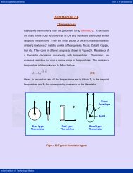
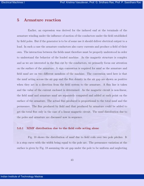
Fig. 18 shows the distribution of mmf due to field coils over two pole pitches. It 

is a step curve with the width being equal to the pole arc. The permeance variation at the 

surface is given by Fig. 18 assuming the air gap under the pole to be uniform and neglecting 

43



N S 

Ideal flux density 

Figure 18: Mmf and flux variation in an unloaded machine 

44 

mmf 

Permeance 

Practical 

Flux density


the slotting of the armature. The no-load flux density curve can be obtained by multiplying 

mmf and permeance. Allowing for the fringing of the flux, the actual flux density curve 

would be as shown under Fig. 18. 

5.0.2 MMF distribution due to armature conductors alone carrying currents 

S-Pole 


N 

N-Pole 

A 

Generator 

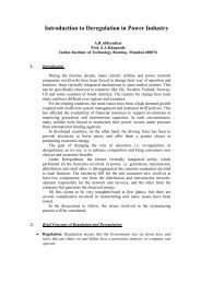
Figure 19: Mmf and flux distribution under the action of armature alone carrying current 

S 

Flux 

mmf 

The armature has a distributed winding, as against the field coils which 

are concentrated and concentric. The mmf of each coil is shifted in space by the number of 

slots. For a full pitched coil, each coil produces a rectangular mmf distribution. The sum 

of the mmf due to all coils would result in a stepped triangular wave form. If we neglect 

slotting and have uniformly spaced coils on the surface, then the mmf distribution due to the 

armature working alone would be a triangular distribution in space since all the conductors 

carry equal currents. MMF distribution is the integral of the ampere conductor distribution. 

45


This is depicted in Fig. 19. This armature mmf per pole is given by 


Fa = 1 

2 .Ic.Z 

2p 

where Ic is the conductor current and Z is total number of conductors on the armature. This 

peak value of the mmf occurs at the inter polar area, shifted from the main pole axis by half 

the pole pitch when the brushes are kept in the magnetic neutral axis of the main poles. 

5.0.3 Total mmf and flux of a loaded machine 

Field 

flux 

b 

Armature flux 

N S 

D 

C 

B 

A 

c 

a 

Brush axis 

A B 

o o’ 

Generator 

Total flux 

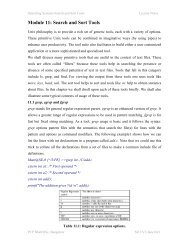
Figure 20: Flux distribution in a loaded generator without brush shift 

The mmf of field coils and armature coils are added up and the re- 

sultant mmf distribution is obtained as shown in Fig. 20. 

46



This shows the decrease in the mmf at one tip of a pole and a substantial rise 

at the other tip. If the machine has a pole arc to pole pitch ratio of 0.7 then 70% of the 

armature reaction mmf gets added at this tip leading to considerable amount of saturation 

under full load conditions. The flux distribution also is shown in Fig. 20. This is obtained 

by multiplying mmf and permeance waves point by point in space. Actual flux distribution 

differs from this slightly due to fringing. As seen from the figure, the flux in the inter polar 

region is substantially lower due to the high reluctance of the medium. The air gaps under 

the pole tips are also increased in practice to reduce excessive saturation of this part. The 

advantage of the salient pole field construction is thus obvious. It greatly mitigates the 

effect of the armature reaction. Also, the coils under going commutation have very little 

emf induced in them and hence better commutation is achieved. Even though the armature 

reaction produced a cross magnetizing effect, the net flux per pole gets slightly reduced, 

on load, due to the saturation under one tip of the pole. This is more so in modern d.c. 

machines where the normal excitation of the field makes the machine work under some level 

of saturation. 

5.0.4 Effect of brush shift 

In some small d.c. machines the brushes are shifted from the position of the mag- 

netic neutral axis in order to improve the commutation. This is especially true of machines 

with unidirectional operation and uni-modal (either as a generator or as a motor) operation. 

Such a shift in the direction of rotation is termed ‘lead’ (or forward lead). Shift of brushes 

in the opposite to the direction of rotation is called ‘backward lead’. This lead is expressed 

in terms of the number of commutator segments or in terms of the electrical angle. A pole 

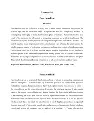
pitch corresponds to an electrical angle of 180 degrees. Fig. 21 shows the effect of a forward 

47


Field 

flux 


b 

a 

N S 

c 

Armature flux 

Geometric Neutral axis 

Brush axis 

Total flux 

(a)Armature reaction with brush shift 

a’ 

b’ 

N 

S 

θ 

b 

Rotation 

(b)Calculation of demagnetizing mmf per pole 

Figure 21: Effect of brush shift on armature reaction 

48 

a 

Rotation


brush lead on the armature reaction. The magnetization action due to the armature is no 

longer entirely cross magnetizing. Some component of the same goes to demagnetize the 

main field and the net useful flux gets reduced. This may be seen as the price we pay for 

improving the commutation. Knowing the pole arc to pole pitch ratio one can determine 

the total mmf at the leading and trailing edges of a pole without shift in the brushes. 


Fmin = Ff − α.Fa 

Fmax = Ff + α.Fa 

where Ff is the field mmf, Fais armature reaction mmf per pole, and α is the pole arc to 

pole pitch ratio. 

Fa = 1 

2 

(22) 

Z.Ic 

. (23) 

2p 

The net flux per pole decreases due to saturation at the trailing edge and 

hence additional ampere turns are needed on the pole to compensate this effect. This may 

be to the tune of 20 percent in the modern d.c. machines. 

The brush shift gives rise to a shift in the axis of the mmf of the armature 

reaction. This can be resolved into two components, one in the quadrature axis and sec- 

ond along the pole axis as shown in Fig. 21.(b) The demagnetizing and cross magnetizing 

component of the armature ampere turn per pole can be written as 

Fd = 2θ 

π .Fa 

Fq = (1 − 2θ 

π ).Fa 

where θ is the angle of lead . In terms of the number of commutator segments they are 

Fd = Cl 

. C 

4p 

IcZ 

4p 

49 

(24) 

(25) 

or Cl 

C .Ic.Z (26)


where, Cl is the brush lead expressed in number of commutator segments. 

5.0.5 Armature reaction in motors 


As discussed earlier, for a given polarity of the field and sense of rotation, the 

motoring and generating modes differ only in the direction of the armature current. Alter- 

natively, for a given sense of armature current, the direction of rotation would be opposite 

for the two modes. The leading and trailing edges of the poles change positions if direction 

of rotation is made opposite. Similarly when the brush leads are considered, a forward lead 

given to a generator gives rise to weakening of the generator field but strengthens the motor 

field and vice-versa. Hence it is highly desirable, even in the case of non-reversing drives, 

to keep the brush position at the geometrical neutral axis if the machine goes through both 

motoring and generating modes. 

The second effect of the armature reaction in the case of motors as well as 

generators is that the induced emf in the coils under the pole tips get increased when a 

pole tip has higher flux density. This increases the stress on the ‘mica’ (micanite) insulation 

used for the commutator, thus resulting in increased chance of breakdown of these insulating 

sheets. To avoid this effect the flux density distribution under the poles must be prevented 

from getting distorted and peaky. 

The third effect of the armature reaction mmf distorting the flux density is 

that the armature teeth experience a heavy degree of saturation in this region. This increases 

the iron losses occurring in the armature in that region. The saturation of the teeth may 

be too great as to have some flux lines to link the thick end plates used for strengthening 

50


the armature. The increase in iron loss could be as high as 50 percent more at full load 

compared to its no-load value. 


The above two effects can be reduced by providing a ’compensating’ mmf at 

N 

Compensating 

winding 

N 

S 

s 

s 

Figure 22: Compensating winding 

Commutating pole 

S 

N 

N 

Main pole 

the same spatial rate as the armature mmf. This is provided by having a compensating 

winding housed on the pole shoe which carries currents that are directly proportional to the 

armature current. The ampere conductors per unit length is maintained identical to that of 

51


+ 

+ + + + + 


N 

compole mmf 

+ + + + + 

Rotation 

+ 

+ 

S 

+ + 

+ 

+ 

+ 

+ 

+ 

mmf of 

compensating 

winding 

Resultant 

mmf 

Armature 

mmf 

Figure 23: Armature reaction with Compensating winding 

52 

Main field 

mmf


the armature. The sign of the ampere conductors is made opposite to the armature. This is 

illustrated in Fig. 22 and Fig. 23 . Since the compensating winding is connected in series with 

the armature, the relationship between armature mmf and the mmf due to compensating 

winding remains proper for all modes of working of the machine. The mmf required to be 

setup by the compensating winding can be found out to be 


Fc = Ic.Z polearc 

. 

4p polepitch 

Under these circumstances the flux density curve remains unaltered under the poles between 

no-load and full load. 

(27) 

The axis of the mmf due to armature and the compensating winding being 

the same and the signs of mmf being opposite to each other the flux density in the region 

of geometric neutral axis gets reduced thus improving the conditions for commutation. One 

can design the compensating winding to completely neutralize the armature reaction mmf. 

Such a design results in overcompensation under the poles. Improvement in commutation 

condition may be achieved simply by providing a commutating pole which sets up a local 

field of proper polarity. It is better not to depend on the compensating winding for improv- 

ing commutation. 

Compensating windings are commonly used in large generators and motors 

operating on weak field working at high loads. 

From the analysis of the phenomenon of armature reaction that takes place 

in a d.c. machine it can be inferred that the equivalent circuit of the machine need not be 

modified to include the armature reaction. The machine can simply be modelled as a voltage 

53


source of internal resistance equal to the armature circuit resistance and a series voltage drop 

equal to the brush contact drop, under steady state. With this circuit model one can arrive 

at the external characteristics of the d.c. machine under different modes of operation. 

5.1 Commutation 


As seen earlier, in an armature conductor of a heteropolar machine a.c. voltages 

are induced as the conductor moves under north and south pole polarities alternately. The 

frequency of this induced emf is given by the product of the pole-pairs and the speed in 

revolutions per second. The induced emf in a full pitch coil changes sign as the coil crosses 

magnetic neutral axis. In order to get maximum d.c. voltage in the external circuit the coil 

should be shifted to the negative group. This process of switching is called commutation. 

During a short interval when the two adjacent commutator segments get bridged by the 

brush the coils connected in series between these two segments get short circuited. Thus in 

the case of ring winding and simple lap winding 2p coils get short circuited. In a simple wave 

winding in a 2p pole machine 2 coils get short circuited. The current in these coils become 

zero and get reversed as the brush moves over to the next commutator segment. Thus brush 

and commutator play an important role in commutation. Commutation is the key process 

which converts the induced a.c. voltages in the conductors into d.c. It is important to learn 

about the working of the same in order to ensure a smooth and trouble free operation of the 

machine. 

54


Entering Edge 

Length 

Width 


Thickness 

Leaving Edge 

3 

2 

2 

2 

1 

2 

x 

(a)Location of Brush (b)Process of commutation 

Figure 24: Location of the brush and Commutation process 

55 

(a) 

(b) 

(c) 

4 

4 

4 

4 

4 

3 

4 

3 

3 

3 

3 

Ia 

I2 

2 

Ia 

Ia 

1 

tb 

tb 

i 

2 

tb 

Ia 

2Ia 

1 

Ia 

1 

2Ia 

1 

2Ia 

Ia 

I1 

2Ia 

1 

2Ia 

Motion


5.1.1 Brushes 


Brush forms an important component in the process of commutation. The coil 

resistance is normally very small compared to the brush contact resistance. Further this 

brush contact resistance is not a constant. With the brushes commonly used, an increase in 

the current density of the brushes by 100 percent increases the brush drop by about 10 to 

15 percent. Brush contact drop is influenced by the major factors like speed of operation, 

pressure on the brushes, and to a smaller extent the direction of current flow. 

Major change in contact resistance is brought about by the composition of 

the brush. Soft graphite brushes working at a current density of about 10A/cm 2 produce a 

drop of 1.6V (at the positive and negative brushes put together) while copper-carbon brush 

working at 15A/cm 2 produces a drop of about 0.3V. The coefficient of friction for these 

brushes are 0.12 and 0.16 respectively. The attention is focussed next on the process of 

commutation. 

5.1.2 Linear Commutation 

If the current density under the brush is assumed to be constant through out the 

commutation interval, a simple model for commutation is obtained. For simplicity, the brush 

thickness is made equal to thickness of one commutator segment. In Fig. 24(b), the brush 

is initially solely resting on segment number 1. The total current of 2Ia is collected by 

the brush as shown. As the commutator moves relative to the brush position, the brush 

position starts to overlap with that of segment 2. As the current density is assumed to be 

constant, the current from each side of the winding is proportional to the area shared on the 

56


two segments. Segment 1 current uniformly comes down with segment 2 current increasing 

uniformly keeping the total current in the brush constant. The currents I1 and I2 in brush 

segments 1 and 2 are given by 

giving I1 + I2 to be 2 Ia. 


I1 = 2Ia(1 − x 

tb 

x 

) and I2 = 2Ia 

tb 

Here ‘x’ is the width of the brush overlapping on segment 2. The process of commutation 

would be over when the current through segment number 1 becomes zero. The current in 

the coil undergoing commutation is 

i = I1 − Ia = Ia − I2 = (I1 − I2) 

2 

The time required to complete this commutation is 

Tc = tb 

(28) 

= Ia(1 − 2x 

) (29) 

where vc is the velocity of the commutator. This type of linear commutation is very close 

to the ideal method of commutation. The time variation of current in the coil undergoing 

commutation is shown in Fig. 25.(a). Fig. 25.(b) also shows the timing diagram for the 

currents I1 and I2 and the current densities in entering edge αe, leaving edge αl and also the 

mean current density αm in the brush. Machines having very low coil inductances, operating 

at low load currents, and low speeds, come close to this method of linear commutation. 

vc 

tb 

(30) 

In general commutation will not be linear due to the presence of emf of self 

induction and induced rotational emf in the coil. These result in retarded and accelerated 

commutation and are discussed in sequence. 

57


Ia 

0 Tc 

Time of 

communication 


i 

Time 

-Ia 

2Ia 

0 

I1 I2 

Time of 

commutation 

(a) (b) 

5.1.3 Retarded commutation 

Figure 25: Linear commutation 

αm = 

Tc 

α’ = α" 

Retarded commutation is mainly due to emf of self induction in the coil. Here 

the current transfer from 1 to 2 gets retarded as the name suggests. This is best explained 

with the help of time diagrams as shown in Fig. 26.(a). The variation of i is the change in 

the current of the coil undergoing commutation, while i ′ 

is that during linear commutation. 

Fig. 26(b) shows the variation of I1 and current density in the brush at the leaving edge and 

Fig. 26.(c) shows the same phenomenon with respect to I2 at entering edge. The value of 

current in the coil is given by i undergoing commutation. αm is the mean current density in 

the brush given by total current divided by brush area of cross section. αl and αe are the 

current density under leaving and entering edges of the brush. As before, 

I1 = Ia + i and I2 = Ia − i (31) 

58


+Ia 


0 

t 

i’ 

i 

Tc 

-Ia 

(a) commutation (b) Leaving edge density 

t 

2Ia 

+Ia 

0 Tc 

E 

F 

D 

I2=Ia-i 

(c)Entry edge density 

2Ia 

α"=DF/DE 

Figure 26: Diagrams for Retarded commutation 

59 

P 

0 

t 

C 

A 

B 

t 

I1=Ia+i 

αm 

α’=AB/AC 

Q 

Tc


The variation of densities at leaving and entering edges are given as 


αl = AB 

AC .αm 

αe = DF 

DE .αm 

At the very end of commutation, the current density 

αe = αm. di 

dt /di′ 

dt 

= αm. di 

dt /2Ia 

Tc 

If at this point di/dt = 0 the possibility of sudden breaking of the current and 

hence the creation of an arc is removed . 

in Fig. 27.(b). 

(32) 

(33) 

(34) 

Similarly at the entering edge at the end of accelerated commutation, shown 

αe = αm. di 

dt /2Ia 

Tc 

Thus retarded communication results in di/dt = 0 at the beginning of commutation 

(at entering edge) and accelerated communication results in the same at the end of commu- 

tation (at leaving edge). Hence it is very advantageous to have retarded commutation at the 

entry time and accelerated commutation in the second half. This is depicted in Fig. 27.(b1). 

It is termed as sinusoidal commutation. 

(35) 

Retarded commutation at entry edge is ensured by the emf of self induction 

which is always present. To obtain an accelerated commutation, the coil undergoing com- 

mutation must have in it an induced emf of such a polarity as that under the pole towards 

which it is moving. Therefore the accelerated commutation can be obtained by i) a forward 

60


Ia 

Ia 


0 

0 

i 

i’ 

Tc 

B 

-Ia 

Ia 

(a1) (a2) 

i 

i’ 

Tc 

time 

-Ia 

Ia 

0 

C 

0 

D 

A 

C 

B 

α ’ 

Entering 

edge 

α " 

i 

αm 

(b1) (b2) 

Figure 27: Accelerated and Sinusoidal commutation 

61 

S 

R 

Q 

P 

α’ 

A 

i’ 

i 

α " 

αm 

α’ =AB/AC 

α"=DB/DC 

Tc 

Tc 

B 

Leaving edge 

α ’ =PR/PQ 

α " =SR/SQ 

-Ia 

time 

-Ia


lead given to the brushes or by ii) having the field of suitable polarity at the position of the 

brush with the help of a small pole called a commutating pole. In a non-inter pole machine 

the brush shift must be changed from forward lead to backward lead depending upon gener- 

ating or motoring operation. As the disadvantages of this brush shifts are to be avoided, it 

is preferable to leave the brushes at geometric neutral axis and provide commutating poles 

of suitable polarity (for a generator the polarity of the pole is the one towards which the 

conductors are moving). The condition of commutation will be worse if commutating poles 

are provided and not excited or they are excited but wrongly. 


The action of the commutating pole is local to the coil undergoing commu- 

tation. It does not disturb the main field distribution. The commutating pole winding 

overpowers the armature mmf locally and establishes the flux of suitable polarity. The com- 

mutating pole windings are connected in series with the armature of a d.c. machine to get 

a load dependent compensation of armature reaction mmf. 

The commutating pole are also known as compole or inter pole. The air gap 

under compole is made large and the width of compole small. The mmf required to be 

produced by compole is obtained by adding to the armature reaction mmf per pole Fa the 

mmf to establish a flux density of required polarity in the air gap under the compole Fcp 

.This would ensure straight line commutation. If sinusoidal commutation is required then 

the second component Fcp is increased by 30 to 50 percent of the value required for straight 

line commutation. 

The compole mmf in the presence of a compensating winding on the poles 

62


will be reduced by Fa * pole arc/pole pitch. This could have been predicted as the axis of 

the compensating winding and armature winding is one and the same. Further, the mmf of 

compensating winding opposes that of the armature reaction. 

5.2 Methods of excitation 


It is seen already that the equivalent circuit model of a d.c. machine becomes very 

simple in view of the fact that the armature reaction is cross magnetizing. Also, the axis 

of compensating mmf and mmf of commutating poles act in quadrature to the main field. 

Thus flux under the pole shoe gets distorted but not diminished (in case the field is not 

saturated). The relative connections of armature, compole and compensating winding are 

unaltered whether the machine is working as a generator or as a motor; whether the load 

is on the machine or not. Hence all these are connected permanently inside the machine. 

The terminals reflect only the additional ohmic drops due to the compole and compensating 

windings. Thus commutating pole winding, and compensating winding add to the resistance 

of the armature circuit and can be considered a part of the same. The armature circuit 

can be simply modelled by a voltage source of internal resistance equal to the armature 

resistance + compole resistance + compensating winding resistance. The brushes behave 

like non-linear resistance; and their effect may be shown separately as an additional constant 

voltage drop equal to the brush drop. 

5.2.1 Excitation circuit 

The excitation for establishing the required field can be of two types a) Permanent 

magnet excitation(PM) b) Electro magnetic excitation. Permanent magnet excitation is 

63



lp 

Field 

coil 


ly 

lg lt lt lg 

lp 

la 

da 

Figure 28: Magnetization of a DC machine 

64 

Yoke 

Pole


employed only in extremely small machines where providing a field coil becomes infeasible. 

Also, permanent magnet excited fields cannot be varied for control purposes. Permanent 

magnets for large machines are either not available or expensive. However, an advantage 

of permanent magnet is that there are no losses associated with the establishment of the field. 


Electromagnetic excitation is universally used. Even though certain amount 

of energy is lost in establishing the field it has the advantages like lesser cost, ease of control. 

The required ampere turns for establishing the desired flux per pole may be 

computed by doing the magnetic circuit calculations. MMF required for the poles, air gap, 

armature teeth, armature core and stator yoke are computed and added. Fig. 28 shows two 

poles of a 4-pole machine with the flux paths marked on it. Considering one complete flux 

loop, the permeance of the different segments can be computed as, 

Where P- permeance 

A- Area of cross section of the part 

mu- permeability of the medium 

l- Length of the part 

P = A.µ/l 

A flux loop traverses a stator yoke, armature yoke, and two numbers each 

of poles, air gap, armature teeth in its path. For an assumed flux density Bg in the pole 

region the flux crossing each of the above regions is calculated. The mmf requirement for 

65


establishing this flux in that region is computed by the expressions 


Flux = mmf . permeance 

= B.A 

From these expressions the mmf required for each and every part in the path of 

the flux is computed and added. This value of mmf is required to establish two poles. It 

is convenient to think of mmf per pole which is nothing but the ampere turns required to 

be produced by a coil wound around one pole. In the case of small machines all this mmf 

is produced by a coil wound around one pole. The second pole is obtained by induction. 

This procedure saves cost as only one coil need be wound for getting a pair of poles. This 

produces an unsymmetrical flux distribution in the machine and hence is not used in larger 

machines. In large machines, half of total mmf is assigned to each pole as the mmf per pole. 

The total mmf required can be produced by a coil having large number of turns but taking a 

small current. Such winding has a high value of resistance and hence a large ohmic drop. It 

can be connected across a voltage source and hence called a shunt winding. Such method of 

excitation is termed as shunt excitation. On the other hand, one could have a few turns of 

large cross section wire carrying heavy current to produce the required ampere turns. These 

windings have extremely small resistance and can be connected in series with a large current 

path such as an armature. Such a winding is called a series winding and the method of 

excitation, series excitation. A d.c. machine can have either of these or both these types of 

excitation. 

These are shown in Fig. 29. When both shunt winding and series winding are 

present, it is called compound excitation. The mmf of the two windings could be arranged to 

aid each other or oppose each other. Accordingly they are called cumulative compounding 

and differential compounding. If the shunt winding is excited by a separate voltage source 

66


F2 

F1 

Diverter 

Shunt field 

S2 

Series 

field 


S1 

A2 

A1 

A2 

A1 

F2 

F1 

Shunt field 

(a)Separate excitation (b) Self excitation 

Long shunt 

Short shunt 

(c)Series excitation (d)Compound excitation 

Figure 29: D.C generator connections 

67 

F2 

F1 

S2 

S1 

A2 

A1 

A2 

A1


then it is called separate excitation. If the excitation power comes from the same machine, 

then it is called self excitation. Series generators can also be separately excited or self excited. 

The characteristics of these generators are discussed now in sequence. 

5.2.2 Separately excited shunt generators 

Prime 

mover 

n=const 


+ 

Vdc 

- 

E 

A2 

A1 

Ia=0 

F2 

F1 

If 

Induced e.m.f 

Decreasing 

Magnetisation 

Increasing 

magnetisation 

e.m.f. due to Residual Magnetism 

(a) (b) 

Figure 30: Magnetization characteristics 

Exciting Current 

Fig. 30 shows a shunt generator with its field connected to a voltage 

source Vf through a regulating resistor in potential divider form. The current drawn by 

the field winding can be regulated from zero to the maximum value. If the change in the 

excitation required is small, simple series connection of a field regulating resistance can be 

used. In all these cases the presence of a prime mover rotating the armature is assumed. A 

68


separate excitation is normally used for testing of d.c. generators to determine their open 

circuit or magnetization characteristic. The excitation current is increased monotonically 

to a maximum value and then decreased in the same manner, while noting the terminal 

voltage of the armature. The load current is kept zero. The speed of the generator is held 

at a constant value. The graph showing the nature of variation of the induced emf as a 

function of the excitation current is called as open circuit characteristic (occ), or no-load 

magnetization curve or no-load saturation characteristic. Fig. 30(b). shows an example. The 

magnetization characteristic exhibits saturation at large values of excitation current. Due 

to the hysteresis exhibited by the iron in the magnetic structure, the induced emf does not 

become zero when the excitation current is reduced to zero. This is because of the remnant 

field in the iron. This residual voltage is about 2 to 5 percent in modern machines. Separate 

excitation is advantageous as the exciting current is independent of the terminal voltage 

and load current and satisfactory operation is possible over the entire voltage range of the 

machine starting from zero. 

5.2.3 Self excitation 


In a self excited machine, there is no external source for providing excitation current. 

The shunt field is connected across the armature. For series machines there is no change in 

connection. The series field continues to be in series with the armature. 

Self excitation is now discussed with the help of Fig. 31.(a) The pro- 

cess of self excitation in a shunt generator takes place in the following manner. When the 

armature is rotated a feeble induced emf of 2 to 5 percent appears across the brushes de- 

pending upon the speed of rotation and the residual magnetism that is present. This voltage 

69


Induced emf on open circuit 

F2 

F1 

200 

160 

120 

80 

40 

A2 

A1 


200 

n 

Prime 

mover 

Open circuit e.m.f,volts 

210 

180 

150 

120 

90 

60 

30 

0 

375 ohms 

280 ohms 

250 ohms 

170 ohms 

140 ohms 

1.0 

Exciting current,Amperes 

(a)Physical connection (b) characteristics 

Critical Resistance 

400 

Total field circuit resistance, ohms 

Open circuit e.m.f,volts 

125 ohms 

speed in rev/min 

(c)Critical resistance (d) Critical speed 

210 

180 

150 

120 

90 

60 

30 

Figure 31: Self excitation 

70 

0 

250 ohms 

1500 

1500 rev/min 

1000 rev/min 

500 rev/min 

60 ohms


Voltage 

O ’ 


D 

P 

P’ 

P1 

R’ 

R 

Q’ 

Q1 

QL 

PL 

0 P" Q" A 

Excitation current If 

Armature current Ia 

Q 

A’ 

C 

RL 

Open circuit 

characteristic 

Armature drop 


Figure 32: External characteristics of a self excited of a shunt generator 

gets applied across the shunt field winding and produces a small mmf. If this mmf is such 

as to aid the residual field then it gets strengthened and produces larger voltage across the 

brushes. It is like a positive feed back. The induced emf gradually increases till the voltage 

induced in the armature is just enough to meet the ohmic drop inside the field circuit. Under 

such situation there is no further increase in the field mmf and the build up of emf also stops. 

If the voltage build up is ‘substantial’, then the machine is said to have ‘self excited’. 

Fig. 31(b) shows the magnetization curve of a shunt generator. The field resistance 

line is also shown by a straight line OC. The point of intersection of the open circuit charac- 

71


teristic (OCC) with the field resistance line, in this case C, represents the voltage build up 

on self excitation. If the field resistance is increased, at one point the resistance line becomes 

a tangent to the OCC. This value of the resistance is called the critical resistance. At this 

value of the field circuit resistance the self excitation suddenly collapses. See Fig. 31(c). In- 

stead of increasing the field resistance if the speed of the machine is reduced then the same 

resistance line becomes a critical resistance at a new speed and the self excitation collapses 

at that speed. In this case, as the speed is taken as the variable, the speed is called the 

critical speed. In the linear portion of the OCC the ordinates are proportional to the speed 

of operation, hence the critical resistance increases as a function of speed Fig. 31.(b) and (d). 


The conditions for self excitation can be listed as below. 

1. Residual field must be present. 

2. The polarity of excitation must aid the residual magnetism. 

3. The field circuit resistance must be below the critical value. 

4. The speed of operation of the machine must be above the critical speed. 

5. The load resistance must be very large. 

discussed below. 

Remedial measures to be taken if the machine fails to self excite are briefly 

1. The residual field will be absent in a brand new, unexcited, machine. The field may 

be connected to a battery in such cases for a few seconds to create a residual field. 

72


2. The polarity of connections have to be set right. The polarity may become wrong 


either by reversed connections or reversed direction of rotation. If the generator had 

been working with armature rotating in clockwise direction before stopping and if one 

tries to self excite the same with counter clockwise direction then the induced emf 

opposes residual field, changing the polarity of connections of the field with respect to 

armature is normally sufficient for this problem. 

3. Field circuit resistance implies all the resistances coming in series with the field winding 

like regulating resistance, contact resistance, drop at the brushes, and the armature 

resistance. Brush contact resistance is normally high at small currents. The dirt on 

the commutator due to dust or worn out mica insulator can increase the total circuit 

resistance enormously. The speed itself might be too low so that the normal field 

resistance itself is very much more than the critical value. So ensuring good speed, 

clean commutator and good connections should normally be sufficient to overcome this 

problem. 

4. Speed must be increased sufficiently to a high value to be above the critical speed. 

5. The load switch must be opened or the load resistance is made very high. 

5.2.4 Self excitation of series generators 

The conditions for self excitation of a series generator remain similar to that of 

a shunt machine. In this case the field circuit resistance is the same as the load circuit 

resistance and hence it must be made very low to help self excitation. To control the field 

mmf a small resistance called diverter is normally connected across the series field. To help 

in the creation of maximum mmf during self excitation any field diverter if present must be 

73



Terminal voltage 

0 

Open circuit 


A 

Q 

S 

R B 

P 

External 


Load Current 

PS=PQ-PR 



Figure 33: External characteristics of a Series Generator 

open circuited.In a series generator load current being the field current of the machine the 

self excitation characteristic or one and the same. This is shown in Fig. 33 

5.2.5 Self excitation of compound generators 

Most of the compound machines are basically shunt machines with the series wind- 

ing doing the act of strengthening/weakening the field on load, depending up on the con- 

nections. In cumulatively compounded machines the mmf of the two fields aid each other 

and in a differentially compounded machine they oppose each other. Due to the presence of 

the shunt winding, the self excitation can proceed as in a shunt machine. A small difference 

exists however depending up on the way the shunt winding is connected to the armature. It 

can be a short shunt connection or a long shunt connection. In long shunt connection the 

shunt field current passes through the series winding also. But it does not affect the process 

of self excitation as the mmf contribution from the series field is negligible. 

74



Both series field winding and shunt field winding are wound around the main 

poles. If there is any need, for some control purposes, to have more excitation windings 

of one type or the other they will also find their place on the main poles. The designed 

field windings must cater to the full range of operation of the machine at nominal armature 

current. As the armature current is cross magnetizing the demagnetization mmf due to pole 

tip saturation alone need be compensated by producing additional mmf by the field. 

The d.c. machines give rise to a variety of external characteristics with consid- 

erable ease. The external characteristics are of great importance in meeting the requirements 

of different types of loads and in parallel operation. The external characteristics, also known 

as load characteristics, of these machines are discussed next. 

5.3 Load characteristics of d.c. generators 

Load characteristics are also known as the external characteristics. External char- 

acteristics expresses the manner in which the output voltage of the generator varies as a 

function of the load current, when the speed and excitation current are held constant. If 

they are not held constant then there is further change in the terminal voltage. The terminal 

voltage V can be expressed in terms of the induced voltage E and armature circuit drop as 

Vb - brush contact drop, V 

Ia - armature current, A 

V = E − IaRa − Vb 

Ra - armature resistance + inter pole winding resistance+ series winding resistance + com- 

75 

(36)



Volts 

0 

Open circuit e.m.f 

Terminal voltage V 

Ohmic Drop IaRa 

C 

B 

A 

Load current,Ia 

Induced e.m.f 

Figure 34: External characteristics of a separately excited shunt generator 

pensating winding resistance. 

As seen from the equation E being function of speed and flux per pole it will 

also change when these are not held constant. Experimentally the external characteristics 

can be determined by conducting a load test. If the external characteristic is obtained by 

subtracting the armature drop from the no-load terminal voltage, it is found to depart from 

the one obtained from the load test. This departure is due to the armature reaction which 

causes a saturation at one tip of each pole. Modern machines are operated under certain 

degree of saturation of the magnetic path. Hence the reduction in the flux per pole with 

load is obvious. The armature drop is an electrical drop and can be found out even when 

the machine is stationary and the field poles are unexcited. Thus there is some slight droop 

in the external characteristics, which is good for parallel operation of the generators. 

76



One could easily guess that the self excited machines have slightly higher droop 

in the external characteristic as the induced emf E drops also due to the reduction in the 

applied voltage to the field. If output voltage has to be held constant then the excitation 

current or the speed can be increased. The former is preferred due to the ease with which it 

can be implemented. As seen earlier, a brush lead gives rise to a load current dependent mmf 

along the pole axis. The value of this mmf magnetizes/demagnetizes the field depending on 

whether the lead is backward or forward. 

5.4 External characteristics of a shunt generator 

For a given no-load voltage a self excited machine will have more voltage drop at 

the terminals than a separately excited machine, as the load is increased. This is due to 

the dependence of the excitation current also on the terminal voltage. After certain load 

current the terminal voltage decreases rapidly along with the terminal current, even when 

load impedance is reduced. The terminal voltage reaches an unstable condition. Also, in a 

self excited generator the no-load terminal voltage itself is very sensitive to the point of inter- 

section of the magnetizing characteristics and field resistance line. The determination of the 

external characteristics of a shunt generator forms an interesting study. If one determines 

the load magnetization curves at different load currents then the external characteristics 

can be easily determined. Load magnetization curve is a plot showing the variation of the 

terminal voltage as a function of the excitation current keeping the speed and armature cur- 

rent constant. If such curves are determined for different load currents then by determining 

the intersection points of these curves with field resistance line one can get the external 

characteristics of a shunt generator. Load saturation curve can be generated from no-load 

saturation curve /OCC by subtracting the armature drop at each excitation point. Thus 

77


it is seen that these family of curves are nothing but OCC shifted downwards by armature 

drop. Determining their intercepts with the field resistance line gives us the requisite result. 

Instead of shifting the OCC downwards, the x axis and the field resistance line is shifted ‘up- 

wards’ corresponding to the drops at the different currents, and their intercepts with OCC 

are found. These ordinates are then plotted on the original plot. This is shown clearly in 

Fig. 32. The same procedure can be repeated with different field circuit resistance to yield 

external characteristics with different values of field resistance. The points of operation up to 

the maximum current represent a stable region of operation. The second region is unstable. 

The decrease in the load resistance decreases the terminal voltage in this region. 

5.4.1 External characteristics of series generators 


In the case of series generators also, the procedure for the determination of the 

external characteristic is the same. From the occ obtained by running the machine as a sep- 

arately excited one, the armature drops are deducted to yield external /load characteristics. 

The armature drop characteristics can be obtained by a short circuit test as before. 

Fig. 33 shows the load characteristics of a series generator. The first half of 

the curve is unstable for constant resistance load. The second half is the region where series 

generator connected to a constant resistance load could work stably. The load characteristics 

in the first half however is useful for operating the series generator as a booster. In a booster 

the current through the machine is decided by the external circuit and the voltage injected 

into that circuit is decided by the series generator. This is shown in Fig. 35 

78


F2 

F1 


E1 

A2 

A1 

Main generator 

S1 S2 

A1 

- + 

E2 

A2 

Booster 

Generator 

Figure 35: Series generator used as Booster 

5.4.2 Load characteristics of compound generators 

E=E1+ 

- 

In the case of compound generators the external characteristics resemble those of 

shunt generators at low loads. The load current flowing through the series winding aids 

or opposes the shunt field ampere turns depending upon whether cumulative or differential 

compounding is used. This increases /decreases the flux per pole and the induced emf E. 

Thus a load current dependant variation in the characteristic occurs. If this increased emf 

cancels out the armature drop the terminal voltage remains practically same between no 

load and full load. This is called as level compounding. Any cumulative compounding below 

this value is called under compounding and those above are termed over- compounding. 

These are shown in Fig. 36. The characteristics corresponding to all levels of differential 

compounding lie below that of a pure shunt machine as the series field mmf opposes that of 

the shunt field. 

79 

E2



F2 

F1 

Vf 


If 

A2 

A1 

S2 

S1 

(a)-Connection 

Load current 

(b)-Characteristics 

IL 

# Prime 

mover 

Over compounded 

Load 

Level compounded 

Under compounded 

Shunt machine 

Differential 

compounding 

Figure 36: External characteristic of Compound Generator 

80



External characteristics for other voltages of operation can be similarly derived 

by changing the speed or the field excitation or both. 

5.5 Parallel operation of generators 

D.C. generators are required to operate in parallel supplying a common load when 

the load is larger than the capacity of any one machine. In situations where the load is small 

but becomes high occasionally, it may be a good idea to press a second machine into operation 

only as the demand increases. This approach reduces the spare capacity requirement and its 

cost. In cases where one machine is taken out for repair or maintenance, the other machine 

can operate with reduced load. In all these cases two or more machines are connected to 

operate in parallel. 

5.5.1 Shunt Generators 

Parallel operation of two shunt generators is similar to the operation of two storage 

batteries in parallel. In the case of generators we can alter the external characteristics easily 

while it is not possible with batteries. Before connecting the two machines the voltages of 

the two machines are made equal and opposing inside the loop formed by the two machines. 

This avoids a circulating current between the machines. The circulating current produces 

power loss even when the load is not connected. In the case of the loaded machine the 

difference in the induced emf makes the load sharing unequal. 

Fig. 37 shows two generators connected in parallel. The no load emfs are made 

equal to E1 = E2 = E on no load; the current delivered by each machine is zero. As the load 

is gradually applied a total load current of I ampere is drawn by the load. The load voltage 

81


Prime 

mover 


Vf1 

F1 

G1 

A2 

A1 

s1 

F2 F2 

v 

Vf2 

F1 

Figure 37: Connection of two shunt generators in Parallel 

V2 k V0 j 

E2 

Terminal 

Voltage 

E1 

V 

O 

I1 

I2 

I=I1+I2 

Load current 

G2 

A2 

A1 

s2 

Total characteristic 

A B C 

Figure 38: Characteristics of two shunt generators in Parallel 

82 

D 

V2 

V1 

Load


under these conditions is V volt. Each machines will share this total current by delivering 

currents of I1 and I2 ampere such that I1 + I2 = I. 


Also terminal voltage of the two machines must also be V volt. This is dictated 

by the internal drop in each machine given by equations 

V = E1 − I1Ra1 = E2 − I2Ra2 

where Ra1 and Ra2 are the armature circuit resistances. If load resistance RL is known these 

equations can be solved analytically to determine I1 and I2 and hence the manner in which 

to total output power is shared. If RL is not known then an iterative procedure has to be 

adopted. A graphical method can be used with advantage when only the total load current is 

known and not the value of RL or V . This is based on the fact that the two machines have a 

common terminal voltage when connected in parallel. In Fig. 38 the external characteristics 

of the two machines are first drawn as I and II . For any common voltage the intercepts OA 

and OB are measured and added and plotted as point at C. Here OC = OA + OB . Thus 

a third characteristics where terminal voltage is function of the load current is obtained. 

This can be called as the resultant or total external characteristics of the two machines put 

together. With this, it is easy to determine the current shared by each machine at any total 

load current I. 

(37) 

The above procedure can be used even when the two voltages of the machines 

at no load are different. At no load the total current I is zero ie I1 + I2 = 0 or I1 = −I2. 

Machine I gives out electrical power and machine II receives the same. Looking at the voltage 

equations, the no load terminal equation Vo becomes 

Vo = E1 − I1nlRa1 = E2 + I2nlRa2 

83 

(38)



As can be seen larger the values of Ra1 and Ra2 larger is the tolerance for the error 

between the voltages E1 and E2. The converse is also true. When Ra1 and Ra2 are nearly zero 

implying an almost flat external characteristic, the parallel operation is extremely difficult. 

5.5.2 Series generators 

Series generators are rarely used in industry for supplying loads. Some applications 

like electric braking may employ them and operate two or more series generates in parallel. 

Fig. 39 shows two series generators connected in parallel supplying load current of I1 and I2. 

If now due to some disturbance E1 becomes E1 + ∆E1 then the excitation of the machine I 

increases, increasing the load current delivered. As the total current is I the current supplied 

by machine II reduces, so also its excitation and induced emf. Thus machine I takes greater 

and greater fraction of the load current with machine II shedding its load. Ultimately the 

current of machine II becomes negative and it also loads the first machine. Virtually there is 

a short circuit of the two sources, the whole process is thus highly unstable. One remedy is 

for a problem as this is to make the two fields immune to the circulating current between the 

machines. This is done by connecting an equalizer between the fields as shown in Fig. 39-a 

. With the equalizer present, a momentary disturbance does not put the two machines out 

of action. A better solution for such problems is to cross connect the two fields as shown in 

Fig. 39-b. A tendency to supply a larger current by a machine strengthens the field of the 

next machine and increases its induced emf . This brings in stable conditions for operation 

rapidly. 

84


A2 

A1 

A2 

A1 


S2 

S1 

S2 

S1 

G1 

- 

+ 

I1 

- 

F1 

I1 I1+I2 

Equaliser 

A2 

A1 

F2 

+ 

I2 

- 

S1 

S2 

I1+I2 

I1+I2 

(a)Equalizer connection 

I1 I2 

A2 

+ 

- 

I2 

I2 

A1 

I1 

G2 

+ 

- 

S2 

S1 - I1+I2 

I1+I2 

(b)Cross connection of fields 

Figure 39: Series Generator working in parallel 

85 

Load 

V 

V


F2 

F1 

F2 

F1 

S1 


+ 

A2 

+ 

A1 

- - 

F1 

S2 

+ 

S1 

A2 

F2 

Equalizer 

A1 

- - 

F1 

S2 

S2 

S1 

A2 

A1 

(a)Equalizer connection 

F2 

+ 

A2 

A1 

S2 

S1 

(b)Cross connection of series fields 

Figure 40: Compound generators operating in parallel 

86 

Load 

Load 

V 

V


5.5.3 Compound Generators 


The parallel operation of compound machines is similar to shunt generators. Dif- 

ferential compounding would produce a drooping external characteristics and satisfactory 

parallel operation is made easy. But most of the generators are used in the cumulatively 

compounded mode. In such cases the external characteristics will be nearly flat making the 

parallel operation more difficult. By employing equalizer connection for the series windings 

this problem can be mitigated. Fig. 40 shows the connection diagram for parallel operation 

of two compound generators. 

5.6 D.C. motors 

D.C. motors have a place of pride as far as electrical drives are considered. The 

simplicity, and linearity of the control method makes them highly preferred machines in 

precision drives. In spite of the great advancements in a.c. drives these machines are still 

sought after by the industries. Apart from high precision application they are preferred in 

stand alone systems working on batteries and high speed drives off constant voltage mains. 

After the field is excited if we pass a current through the armature the rotor experiences 

a torque and starts rotating. The direction of the torque can be readily obtained from the 

law of interaction. These moving conductors cut the field and induce emf, usually called the 

’back emf’ according to Lenz’s law and act as a sink of electrical power from the electrical 

source. This absorbed power appears as mechanical power. The converted mechanical power 

should overcome the frictional and iron losses before useful work could be done by the same. 

The connections to the supply of a d.c. shunt motor are given in Fig. 41. 

87


F2 

F1 


A2 

A1 

+ 

- 

(a)Separate excitation (b) Shunt excitation 

F2 

F1 

A2 

A1 

s2 

F2 

F1 

s1 

(c)Practical arrangement 

Figure 41: Shunt motor connections 

88 

+ 

- 

A2 

A1 

DC 

Supply 

+ 

-



Commonly used connection is where in both the field and the armature are 

energized simultaneously Fig. 41(b). As the field has higher inductance and time constant 

torque takes some time to reach the full value corresponding to a given armature current. 

In Fig. 41.(c), the switch S1 is closed a few seconds prior to switch S2 . By then the field 

current would have reached the steady value. So the torque per ampere is high in this case. 

The only difference in the second connection Fig. 41.(a) is that the shunt field 

winding is connected to a separate source. This connection is used when the armature and 

field voltage are different as is common in high voltage d.c. machines. The field voltage is 

kept low in such cases for the sake of control purposes. Here again the field circuit must 

be energized prior to the armature. Suitable interlock should be provided to prevent the 

armature switch being closed prior to / without closing of field circuit as the armature 

currents reach very large values still not producing any torque or rotation. The relevant 

equations for the motoring operation can be written as below 

where 

TL- Load torque 

TM- Motor torque 

J - polar moment of inertia. 

w - angular velocity = 2π.n 

V − E − IaRa − Vb = 0 or E = V − IaRa − Vb (39) 

E = p.φ.Z.n 

b 

TM = 1 

2π .p.φ.ZIa 

b 

and TM − TL = J dw 

dt 

= Keφ.n where Ke = pZ 

b 

= KtφIa where Kt = 1 

2π .pZ 

b 

89 

(40) 

(41) 

(42)



The first one is an electrical equation, the second and the third are electro 

mechanical in nature and the last equation is the mechanical equation of motion. Ke and 

Kt are normally termed as back emf constant and torque constant respectively. Under 

steady speed of operation the fourth equation is not required. Using these equations one 

can determine the torque speed characteristics of the machine for a given applied voltage. 

These characteristics are similar to the external characteristics for a generator. Here the 

torque on the machine is assumed to be varying and the corresponding speed of operation 

is determined. This is termed as the torque speed characteristic of the motor. 

5.7 Torque speed characteristics of a shunt motor 

A constant applied voltage V is assumed across the armature. As the armature 

current Ia, varies the armature drop varies proportionally and one can plot the variation of 

the induced emf E. The mmf of the field is assumed to be constant. The flux inside the 

machine however slightly falls due to the effect of saturation and due to armature reaction. 

The variation of these parameters are shown in Fig. 42. 

Knowing the value of E and flux one can determine the value of the speed. 

Also knowing the armature current and the flux, the value of the torque is found out. This 

procedure is repeated for different values of the assumed armature currents and the values 

are plotted as in Fig. 42-(a). From these graphs, a graph indicating speed as a function of 

torque or the torque-speed characteristics is plotted Fig. 42-(b)(i). 

As seen from the figure the fall in the flux due to load increases the speed due 

to the fact that the induced emf depends on the product of speed and flux. Thus the speed 

90


Flux, Speed and Torque 


Line voltage 

A No load speed B 

Speed 

E 

0 

Speed 

0 

Armature current 

C 

F 

Torque Flux 

(a)Load characteristics 

Torque 

(b)Torque speed curve 

Figure 42: DC Shunt motor characteristics 

91 

G 

Back emf 

(ii) 

(i)


of the machine remains more or less constant with load. With highly saturated machines 

the on-load speed may even slightly increase at over load conditions. This effects gets more 

pronounced if the machine is designed to have its normal field ampere turns much less 

than the armature ampere turns. This type of external characteristics introduces instability 

during operation Fig. 42(b)(ii) and hence must be avoided. This may be simply achieved by 

providing a series stability winding which aids the shunt field mmf. 

5.8 Load characteristics of a series motor 


Following the procedure described earlier under shunt motor, the torque speed 

characteristics of a series motor can also be determined. The armature current also happens 

to be the excitation current of the series field and hence the flux variation resembles the 

magnetization curve of the machine. At large value of the armature currents the useful flux 

would be less than the no-load magnetization curve for the machine. Similarly for small 

values of the load currents the torque varies as a square of the armature currents as the flux 

is proportional to armature current in this region. As the magnetic circuit becomes more 

and more saturated the torque becomes proportional to Ia as flux variation becomes small. 

Fig. 43(a) shows the variation of E1, flux , torque and speed following the above procedure 

from which the torque-speed characteristics of the series motor for a given applied voltage 

V can be plotted as shown in Fig. 43.(b) The initial portion of this torque-speed curve is 

seen to be a rectangular hyperbola and the final portion is nearly a straight line. The speed 

under light load conditions is many times more than the rated speed of the motor. Such 

high speeds are unsafe, as the centrifugal forces acting on the armature and commutator 

can destroy them giving rise to a catastrophic break down. Hence series motors are not 

recommended for use where there is a possibility of the load becoming zero. In order to 

92


Torque, Flux and Speed 


Speed 

0 

Back emf 

No load 

Magnetisation 

curve 


Developed 

Torque 

Load current 

(a)Load characteristics 

Torque 

(b)-Torque speed curve 

Useful 

Flux 

Useful 

Torque 

Speed 

Figure 43: Load characteristics of a Series Motor 

93


safeguard the motor and personnel, in the modern machines, a ‘weak’ shunt field is provided 

on series motors to ensure a definite, though small, value of flux even when the armature 

current is nearly zero. This way the no-load speed is limited to a safe maximum speed. It is 

needless to say, this field should be connected so as to aid the series field. 

5.9 Load characteristics of a compound motor 


Two situations arise in the case of compound motors. The mmf of the shunt field 

and series field may oppose each other or they may aid each other. The first configuration 

is called differential compounding and is rarely used. They lead to unstable operation of 

the machine unless the armature mmf is small and there is no magnetic saturation. This 

mode may sometimes result due to the motoring operation of a level-compounded generator, 

say by the failure of the prime mover. Also, differential compounding may result in large 

negative mmf under overload/starting condition and the machine may start in the reverse 

direction. In motors intended for constant speed operation the level of compounding is very 

low as not to cause any problem. 

Cumulatively compounded motors are very widely used for industrial drives. 

High degree of compounding will make the machine approach a series machine like charac- 

teristics but with a safe no-load speed. The major benefit of the compounding is that the 

field is strengthened on load. Thus the torque per ampere of the armature current is made 

high. This feature makes a cumulatively compounded machine well suited for intermittent 

peak loads. Due to the large speed variation between light load and peak load conditions, a 

fly wheel can be used with such motors with advantage. Due to the reasons provided under 

shunt and series motors for the provision of an additional series/shunt winding, it can be 

94


seen that all modern machines are compound machines. The difference between them is only 

in the level of compounding. 


95

5 Armature reaction - nptel - Indian Institute of Technology Madras

Create successful ePaper yourself

Delete template?

Save as template?