15.4 General Linear Least Squares

More documents

Recommendations

Info

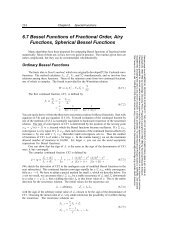
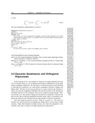
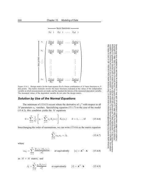
666 Chapter 15. Modeling of Data data points x1 x2 . xN X1( ) X2( ) . . . XM( ) X1(x1) σ1 X1(x2) σ2 . . . X1(xN) σN basis functions X2(x1) σ1 X2(x2) σ2 X2(xN) σN . . . XM(x1) σ1 . . . XM(x2) σ2 . . . . . . . . XM(xN) σN Figure 15.4.1. Design matrix for the least-squares fit of a linear combination of M basis functions to N data points. The matrix elements involve the basis functions evaluated at the values of the independent variable at which measurements are made, and the standard deviations of the measured dependent variable. The measured values of the dependent variable do not enter the design matrix. Solution by Use of the Normal Equations The minimum of (15.4.3) occurs where the derivative of χ 2 with respect to all M parameters ak vanishes. Specializing equation (15.1.7) to the case of the model (15.4.2), this condition yields the M equations ⎡ ⎤ N 0= 1 M ⎣yi − ajXj(xi) ⎦ Xk(xi) k =1,...,M (15.4.6) σ i=1 2 i j=1 Interchanging the order of summations, we can write (15.4.6) as the matrix equation where αkj = N i=1 Xj(xi)Xk(xi) σ 2 i an M × M matrix, and βk = N i=1 yiXk(xi) σ 2 i M j=1 αkjaj = βk (15.4.7) or equivalently [α] =A T · A (15.4.8) or equivalently [β] =A T · b (15.4.9) Sample page from NUMERICAL RECIPES IN FORTRAN 77: THE ART OF SCIENTIFIC COMPUTING (ISBN 0-521-43064-X) Copyright (C) 1986-1992 by Cambridge University Press. Programs Copyright (C) 1986-1992 by Numerical Recipes Software. Permission is granted for internet users to make one paper copy for their own personal use. Further reproduction, or any copying of machinereadable files (including this one) to any server computer, is strictly prohibited. To order Numerical Recipes books or CDROMs, visit website http://www.nr.com or call 1-800-872-7423 (North America only), or send email to directcustserv@cambridge.org (outside North America).
15.4 General Linear Least Squares 667 a vector of length M. The equations (15.4.6) or (15.4.7) are called the normal equations of the leastsquares problem. They can be solved for the vector of parameters a by the standard methods of Chapter 2, notably LU decomposition and backsubstitution, Choleksy decomposition, or Gauss-Jordan elimination. In matrix form, the normal equations can be written as either [α] · a =[β] or as A T · A · a = A T · b (15.4.10) The inverse matrix Cjk ≡ [α] −1 jk is closely related to the probable (or, more precisely, standard) uncertainties of the estimated parameters a. To estimate these uncertainties, consider that aj = M [α] −1 k=1 M jk βk = Cjk k=1 N i=1 yiXk(xi) σ2 i (15.4.11) and that the variance associated with the estimate aj can be found as in (15.2.7) from σ 2 (aj) = N i=1 Note that αjk is independent of yi, so that Consequently, we find that σ 2 (aj) = M M ∂aj = ∂yi M k=1 l=1 CjkCjl σ 2 i ∂aj ∂yi 2 CjkXk(xi)/σ k=1 2 i N i=1 Xk(xi)Xl(xi) σ2 i (15.4.12) (15.4.13) (15.4.14) The final term in brackets is just the matrix [α]. Since this is the matrix inverse of [C], (15.4.14) reduces immediately to σ 2 (aj) =Cjj (15.4.15) In other words, the diagonal elements of [C] are the variances (squared uncertainties) of the fitted parameters a. It should not surprise you to learn that the off-diagonal elements Cjk are the covariances between aj and ak (cf. 15.2.10); but we shall defer discussion of these to §15.6. We will now give a routine that implements the above formulas for the general linear least-squares problem, by the method of normal equations. Since we wish to compute not only the solution vector a but also the covariance matrix [C], it is most convenient to use Gauss-Jordan elimination (routine gaussj of §2.1) to perform the linear algebra. The operation count, in this application, is no larger than that for LU decomposition. If you have no need for the covariance matrix, however, you can save a factor of 3 on the linear algebra by switching to LU decomposition, without Sample page from NUMERICAL RECIPES IN FORTRAN 77: THE ART OF SCIENTIFIC COMPUTING (ISBN 0-521-43064-X) Copyright (C) 1986-1992 by Cambridge University Press. Programs Copyright (C) 1986-1992 by Numerical Recipes Software. Permission is granted for internet users to make one paper copy for their own personal use. Further reproduction, or any copying of machinereadable files (including this one) to any server computer, is strictly prohibited. To order Numerical Recipes books or CDROMs, visit website http://www.nr.com or call 1-800-872-7423 (North America only), or send email to directcustserv@cambridge.org (outside North America).
Page 1: 15.4 General Linear Least Squares 6
Page 5 and 6: 15.4 General Linear Least Squares 6
Page 11: do 11 j=3,nl f1=d f2=f2+twox d=d+1.

15.4 General Linear Least Squares

You also want an ePaper? Increase the reach of your titles

Delete template?

Save as template?