15.4 General Linear Least Squares

15.4 General Linear Least Squares 665 

15.4 General Linear Least Squares 

An immediate generalization of §15.2 is to fit a set of data points (x i, yi) to a 

model that is not just a linear combination of 1 and x (namely a + bx), but rather a 

linear combination of any M specified functions of x. For example, the functions 

could be 1,x,x 2 ,...,x M−1 , in which case their general linear combination, 

(15.4.1) 

is a polynomial of degree M − 1. Or, the functions could be sines and cosines, in 

which case their general linear combination is a harmonic series. 

The general form of this kind of model is 

M 

y(x) = akXk(x) (15.4.2) 

y(x) =a1 + a2x + a3x 2 + ···+ aM x M−1 

i=1 

k=1 

where X1(x),...,XM(x) are arbitrary fixed functions of x, called the basis 

functions. 

Note that the functions Xk(x) can be wildly nonlinear functions of x. In this 

discussion “linear” refers only to the model’s dependence on its parameters a k. 

For these linear models we generalize the discussion of the previous section 

by defining a merit function 

χ 2 N 

 

yi − 

= 

M k=1 akXk(xi) 

2 (15.4.3) 

As before, σi is the measurement error (standard deviation) of the ith data point, 

presumed to be known. If the measurement errors are not known, they may all (as 

discussed at the end of §15.1) be set to the constant value σ =1. 

Once again, we will pick as best parameters those that minimize χ 2 . There are 

several different techniques available for finding this minimum. Two are particularly 

useful, and we will discuss both in this section. To introduce them and elucidate 

their relationship, we need some notation. 

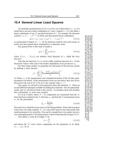
Let A be a matrix whose N × M components are constructed from the M 

basis functions evaluated at the N abscissas xi, and from the N measurement errors 

σi, by the prescription 

Aij = Xj(xi) 


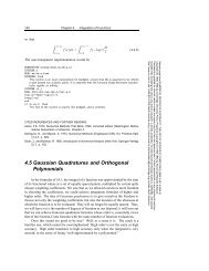
The matrix A is called the design matrix of the fitting problem. Notice that in general 

A has more rows than columns, N ≥M, since there must be more data points than 

model parameters to be solved for. (You can fit a straight line to two points, but not a 

very meaningful quintic!) The design matrix is shown schematically in Figure 15.4.1. 

Also define a vector b of length N by 

σi 

σi 

bi = yi 

σi 


and denote the M vector whose components are the parameters to be fitted, 

a1,...,aM, by a. 

Sample page from NUMERICAL RECIPES IN FORTRAN 77: THE ART OF SCIENTIFIC COMPUTING (ISBN 0-521-43064-X) 

Copyright (C) 1986-1992 by Cambridge University Press. Programs Copyright (C) 1986-1992 by Numerical Recipes Software. 

Permission is granted for internet users to make one paper copy for their own personal use. Further reproduction, or any copying of machinereadable 

files (including this one) to any server computer, is strictly prohibited. To order Numerical Recipes books or CDROMs, visit website 

http://www.nr.com or call 1-800-872-7423 (North America only), or send email to directcustserv@cambridge.org (outside North America).

666 Chapter 15. Modeling of Data 

data points 

x1 

x2 

. 

xN 

X1( ) X2( ) . . . XM( ) 

X1(x1) 

σ1 

X1(x2) 

σ2 

. 

. 

. 

X1(xN) 

σN 

basis functions 

X2(x1) 

σ1 

X2(x2) 

σ2 

X2(xN) 

σN 

. . . XM(x1) 

σ1 

. . . XM(x2) 

σ2 

. 

. 

. 

. 

. 

. . . XM(xN) 

σN 

Figure 15.4.1. Design matrix for the least-squares fit of a linear combination of M basis functions to N 

data points. The matrix elements involve the basis functions evaluated at the values of the independent 

variable at which measurements are made, and the standard deviations of the measured dependent variable. 

The measured values of the dependent variable do not enter the design matrix. 

Solution by Use of the Normal Equations 

The minimum of (15.4.3) occurs where the derivative of χ 2 with respect to all 

M parameters ak vanishes. Specializing equation (15.1.7) to the case of the model 

(15.4.2), this condition yields the M equations 

⎡ 

⎤ 

N 

0= 

1 

M 

⎣yi − ajXj(xi) ⎦ Xk(xi) k =1,...,M (15.4.6) 

σ 

i=1 

2 i 

j=1 

Interchanging the order of summations, we can write (15.4.6) as the matrix equation 

where 

αkj = 

N 

i=1 

Xj(xi)Xk(xi) 

σ 2 i 

an M × M matrix, and 

βk = 

N 

i=1 

yiXk(xi) 

σ 2 i 

M 

j=1 

αkjaj = βk 


or equivalently [α] =A T · A (15.4.8) 

or equivalently [β] =A T · b (15.4.9) 







a vector of length M. 

The equations (15.4.6) or (15.4.7) are called the normal equations of the leastsquares 

problem. They can be solved for the vector of parameters a by the standard 

methods of Chapter 2, notably LU decomposition and backsubstitution, Choleksy 

decomposition, or Gauss-Jordan elimination. In matrix form, the normal equations 

can be written as either 

[α] · a =[β] or as 

A T · A · a = A T · b (15.4.10) 

The inverse matrix Cjk ≡ [α] −1 

jk is closely related to the probable (or, more 

precisely, standard) uncertainties of the estimated parameters a. To estimate these 

uncertainties, consider that 

aj = 

M 

[α] −1 

k=1 

M 

jk βk = Cjk 

k=1 

N 

i=1 

yiXk(xi) 

σ2 

i 


and that the variance associated with the estimate aj can be found as in (15.2.7) from 

σ 2 (aj) = 

N 

i=1 

Note that αjk is independent of yi, so that 

Consequently, we find that 

σ 2 (aj) = 

M 

M ∂aj 

= 

∂yi 

M 

k=1 l=1 

CjkCjl 

σ 2 i 

∂aj 

∂yi 

2 

CjkXk(xi)/σ 

k=1 

2 i 

N 

i=1 

Xk(xi)Xl(xi) 

σ2 

i 




The final term in brackets is just the matrix [α]. Since this is the matrix inverse of 

[C], (15.4.14) reduces immediately to 

σ 2 (aj) =Cjj 


In other words, the diagonal elements of [C] are the variances (squared 

uncertainties) of the fitted parameters a. It should not surprise you to learn that the 

off-diagonal elements Cjk are the covariances between aj and ak (cf. 15.2.10); but 

we shall defer discussion of these to §15.6. 

We will now give a routine that implements the above formulas for the general 

linear least-squares problem, by the method of normal equations. Since we wish to 

compute not only the solution vector a but also the covariance matrix [C], it is most 

convenient to use Gauss-Jordan elimination (routine gaussj of §2.1) to perform the 

linear algebra. The operation count, in this application, is no larger than that for LU 

decomposition. If you have no need for the covariance matrix, however, you can 

save a factor of 3 on the linear algebra by switching to LU decomposition, without 







computation of the matrix inverse. In theory, since A T · A is positive definite, 

Cholesky decomposition is the most efficient way to solve the normal equations. 

However, in practice most of the computing time is spent in looping over the data 

to form the equations, and Gauss-Jordan is quite adequate. 

We need to warn you that the solution of a least-squares problem directly from 

the normal equations is rather susceptible to roundoff error. An alternative, and 

preferred, technique involves QR decomposition (§2.10, §11.3, and §11.6) of the 

design matrix A. This is essentially what we did at the end of §15.2 for fitting data to 

a straight line, but without invoking all the machinery of QR to derive the necessary 

formulas. Later in this section, we will discuss other difficulties in the least-squares 

problem, for which the cure is singular value decomposition (SVD), of which we give 

an implementation. It turns out that SVD also fixes the roundoff problem, so it is our 

recommended technique for all but “easy” least-squares problems. It is for these easy 

problems that the following routine, which solves the normal equations, is intended. 

The routine below introduces one bookkeeping trick that is quite useful in 

practical work. Frequently it is a matter of “art” to decide which parameters a k 

in a model should be fit from the data set, and which should be held constant at 

fixed values, for example values predicted by a theory or measured in a previous 

experiment. One wants, therefore, to have a convenient means for “freezing” 

and “unfreezing” the parameters ak. In the following routine the total number of 

parameters ak is denoted ma (called M above). As input to the routine, you supply 

an array ia(1:ma), whose components are either zero or nonzero (e.g., 1). Zeros 

indicate that you want the corresponding elements of the parameter vector a(1:ma) 

to be held fixed at their input values. Nonzeros indicate parameters that should be 

fitted for. On output, any frozen parameters will have their variances, and all their 

covariances, set to zero in the covariance matrix. 

SUBROUTINE lfit(x,y,sig,ndat,a,ia,ma,covar,npc,chisq,funcs) 

INTEGER ma,ia(ma),npc,ndat,MMAX 

REAL chisq,a(ma),covar(npc,npc),sig(ndat),x(ndat),y(ndat) 

EXTERNAL funcs 

PARAMETER (MMAX=50) Set to the maximum number of coefficients ma. 

C USES covsrt,gaussj 

Given a set of data points x(1:ndat), y(1:ndat) with individual standard deviations 

sig(1:ndat), useχ2minimization to fit for some or all of the coefficients a(1:ma) of a 

function that depends linearly on a, y = 

i ai ×afunci(x). The input array ia(1:ma) indicates 

by nonzero entries those components of a that should be fitted for, and by zero entries 

those components that should be held fixed at their input values. The program returns values 

for a(1:ma), χ2 = chisq, and the covariance matrix covar(1:ma,1:ma). (Parameters 

held fixed will return zero covariances.) npc is the physical dimension of covar(npc,npc) 

in the calling routine. The user supplies a subroutine funcs(x,afunc,ma) that returns 

the ma basis functions evaluated at x = x in the array afunc. 

INTEGER i,j,k,l,m,mfit 

REAL sig2i,sum,wt,ym,afunc(MMAX),beta(MMAX) 

mfit=0 

do 11 j=1,ma 

if(ia(j).ne.0) mfit=mfit+1 

enddo 11 

if(mfit.eq.0) pause ’lfit: no parameters to be fitted’ 

do 13 j=1,mfit Initialize the (symmetric) matrix. 

do 12 k=1,mfit 

covar(j,k)=0. 

enddo 12 

beta(j)=0. 

enddo 13 







do 17 i=1,ndat Loop over data to accumulate coefficients of the normal 

call funcs(x(i),afunc,ma) 

ym=y(i) 

equations. 

if(mfit.lt.ma) then Subtract off dependences on known pieces of the fitting 

do 14 j=1,ma 

function. 

if(ia(j).eq.0) ym=ym-a(j)*afunc(j) 

enddo 14 

endif 

sig2i=1./sig(i)**2 

j=0 

do 16 l=1,ma 

if (ia(l).ne.0) then 

j=j+1 

wt=afunc(l)*sig2i 

k=0 

do 15 m=1,l 

if (ia(m).ne.0) then 

k=k+1 

covar(j,k)=covar(j,k)+wt*afunc(m) 

endif 

enddo 15 

beta(j)=beta(j)+ym*wt 

endif 

enddo 16 

enddo 17 

do 19 j=2,mfit Fill in above the diagonal from symmetry. 

do 18 k=1,j-1 

covar(k,j)=covar(j,k) 

enddo 18 

enddo 19 

call gaussj(covar,mfit,npc,beta,1,1) 

j=0 

Matrix solution. 

do 21 l=1,ma 

if(ia(l).ne.0) then 

j=j+1 

a(l)=beta(j) 

endif 

enddo 21 

Partition solution to appropriate coefficients a. 

chisq=0. Evaluate χ2 of the fit. 

do 23 i=1,ndat 


sum=0. 

do 22 j=1,ma 

sum=sum+a(j)*afunc(j) 

enddo 22 

chisq=chisq+((y(i)-sum)/sig(i))**2 

enddo 23 

call covsrt(covar,npc,ma,ia,mfit) Sort covariance matrix to true order of fitting 

return 

END 

coefficients. 

That last call to a subroutine covsrt is only for the purpose of spreading 

the covariances back into the full ma × ma covariance matrix, in the proper rows 

and columns and with zero variances and covariances set for variables which were 

held frozen. 

The subroutine covsrt is as follows. 

SUBROUTINE covsrt(covar,npc,ma,ia,mfit) 

INTEGER ma,mfit,npc,ia(ma) 

REAL covar(npc,npc) 

Expand in storage the covariance matrix covar, so as to take into account parameters that 

are being held fixed. (For the latter, return zero covariances.) 

INTEGER i,j,k 

REAL swap 







do 12 i=mfit+1,ma 

do 11 j=1,i 

covar(i,j)=0. 

covar(j,i)=0. 

enddo 11 

enddo 12 

k=mfit 

do 15 j=ma,1,-1 

if(ia(j).ne.0)then 

do 13 i=1,ma 

swap=covar(i,k) 

covar(i,k)=covar(i,j) 

covar(i,j)=swap 

enddo 13 

do 14 i=1,ma 

swap=covar(k,i) 

covar(k,i)=covar(j,i) 

covar(j,i)=swap 

enddo 14 

k=k-1 

endif 

enddo 15 

return 

END 

Solution by Use of Singular Value Decomposition 

In some applications, the normal equations are perfectly adequate for linear 

least-squares problems. However, in many cases the normal equations are very close 

to singular. A zero pivot element may be encountered during the solution of the 

linear equations (e.g., in gaussj), in which case you get no solution at all. Or a 

very small pivot may occur, in which case you typically get fitted parameters a k 

with very large magnitudes that are delicately (and unstably) balanced to cancel out 

almost precisely when the fitted function is evaluated. 

Why does this commonly occur? The reason is that, more often than experimenters 

would like to admit, data do not clearly distinguish between two or more of 

the basis functions provided. If two such functions, or two different combinations 

of functions, happen to fit the data about equally well — or equally badly — then 

the matrix [α], unable to distinguish between them, neatly folds up its tent and 

becomes singular. There is a certain mathematical irony in the fact that least-squares 

problems are both overdetermined (number of data points greater than number of 

parameters) and underdetermined (ambiguous combinations of parameters exist); 

but that is how it frequently is. The ambiguities can be extremely hard to notice 

a priori in complicated problems. 

Enter singular value decomposition (SVD). This would be a good time for you 

to review the material in §2.6, which we will not repeat here. In the case of an 

overdetermined system, SVD produces a solution that is the best approximation in 

the least-squares sense, cf. equation (2.6.10). That is exactly what we want. In the 

case of an underdetermined system, SVD produces a solution whose values (for us, 

the ak’s) are smallest in the least-squares sense, cf. equation (2.6.8). That is also 

what we want: When some combination of basis functions is irrelevant to the fit, that 

combination will be driven down to a small, innocuous, value, rather than pushed 

up to delicately canceling infinities. 







In terms of the design matrix A (equation 15.4.4) and the vector b (equation 

15.4.5), minimization of χ 2 in (15.4.3) can be written as 

find a that minimizes χ 2 = |A · a − b| 2 


Comparing to equation (2.6.9), we see that this is precisely the problem that routines 

svdcmp and svbksb are designed to solve. The solution, which is given by equation 

(2.6.12), can be rewritten as follows: If U and V enter the SVD decomposition 

of A according to equation (2.6.1), as computed by svdcmp, then let the vectors 

U (i) i =1,...,M denote the columns of U (each one a vector of length N); and 

let the vectors V (i); i =1,...,M denote the columns of V (each one a vector 

of length M). Then the solution (2.6.12) of the least-squares problem (15.4.16) 

can be written as 

a = 

M 

 

U(i) · b 

i=1 

wi 

V (i) 


where the wi are, as in §2.6, the singular values returned by svdcmp. 

Equation (15.4.17) says that the fitted parameters a are linear combinations of 

the columns of V, with coefficients obtained by forming dot products of the columns 

of U with the weighted data vector (15.4.5). Though it is beyond our scope to prove 

here, it turns out that the standard (loosely, “probable”) errors in the fitted parameters 

are also linear combinations of the columns of V. In fact, equation (15.4.17) can 

be written in a form displaying these errors as 

 

M 

U(i) · b 

a = 

i=1 

wi 

V (i) 

 

± 1 

V (1) ±···± 

w1 

1 

V (M) 

wM 


Here each ± is followed by a standard deviation. The amazing fact is that, 

decomposed in this fashion, the standard deviations are all mutually independent 

(uncorrelated). Therefore they can be added together in root-mean-square fashion. 

What is going on is that the vectors V (i) are the principal axes of the error ellipsoid 

of the fitted parameters a (see §15.6). 

It follows that the variance in the estimate of a parameter a j is given by 

σ 2 (aj) = 

M 1 

w 

i=1 

2 [V (i)] 

i 

2 M 

2 Vji 

j = 

wi 

i=1 


whose result should be identical with (15.4.14). As before, you should not be 

surprised at the formula for the covariances, here given without proof, 

Cov(aj,ak) = 

M 

i=1 

VjiVki 

w 2 i 

 


We introduced this subsection by noting that the normal equations can fail 

by encountering a zero pivot. We have not yet, however, mentioned how SVD 

overcomes this problem. The answer is: If any singular value w i is zero, its 







reciprocal in equation (15.4.18) should be set to zero, not infinity. (Compare the 

discussion preceding equation 2.6.7.) This corresponds to adding to the fitted 

parameters a a zero multiple, rather than some random large multiple, of any linear 

combination of basis functions that are degenerate in the fit. It is a good thing to do! 

Moreover, if a singular value wi is nonzero but very small, you should also 

define its reciprocal to be zero, since its apparent value is probably an artifact of 

roundoff error, not a meaningful number. A plausible answer to the question “how 

small is small?” is to edit in this fashion all singular values whose ratio to the 

largest singular value is less than N times the machine precision ɛ. (You might 

argue for √ N, or a constant, instead of N as the multiple; that starts getting into 

hardware-dependent questions.) 

There is another reason for editing even additional singular values, ones large 

enough that roundoff error is not a question. Singular value decomposition allows 

you to identify linear combinations of variables that just happen not to contribute 

much to reducing the χ 2 of your data set. Editing these can sometimes reduce the 

probable error on your coefficients quite significantly, while increasing the minimum 

χ 2 only negligibly. We will learn more about identifying and treating such cases 

in §15.6. In the following routine, the point at which this kind of editing would 

occur is indicated. 

Generally speaking, we recommend that you always use SVD techniques instead 

of using the normal equations. SVD’s only significant disadvantage is that it requires 

an extra array of size N × M to store the whole design matrix. This storage 

is overwritten by the matrix U. Storage is also required for the M × M matrix 

V, but this is instead of the same-sized matrix for the coefficients of the normal 

equations. SVD can be significantly slower than solving the normal equations; 

however, its great advantage, that it (theoretically) cannot fail, more than makes up 

for the speed disadvantage. 

In the routine that follows, the matrices u,v and the vector w are input as working 

space. np and mp are their various physical dimensions. The logical dimensions of the 

problem are ndata data points by ma basis functions (and fitted parameters). If you 

care only about the values a of the fitted parameters, then u,v,w contain no useful 

information on output. If you want probable errors for the fitted parameters, read on. 

SUBROUTINE svdfit(x,y,sig,ndata,a,ma,u,v,w,mp,np, 

* chisq,funcs) 

INTEGER ma,mp,ndata,np,NMAX,MMAX 

REAL chisq,a(ma),sig(ndata),u(mp,np),v(np,np),w(np), 

* x(ndata),y(ndata),TOL 

EXTERNAL funcs 

PARAMETER (NMAX=1000,MMAX=50,TOL=1.e-5) 

NMAX is the maximum expected value of ndata; MMAX the maximum expected for ma; the 

default TOL value is appropriate for single precision and variables scaled to be of order unity. 

C USES svbksb,svdcmp 

Given a set of data points x(1:ndata),y(1:ndata) with individual standard deviations 

sig(1:ndata), useχ2minimization to determine the ma coefficients a of the fitting function 

y = 

i ai×afunci(x). Here we solve the fitting equations using singular value decomposition 

of the ndata by ma matrix, as in §2.6. Arrays u(1:mp,1:np),v(1:np,1:np), 

w(1:np) provide workspace on input; on output they define the singular value decomposition, 

and can be used to obtain the covariance matrix. mp,np are the physical dimensions 

of the matrices u,v,w, as indicated above. It is necessary that mp≥ndata, np ≥ ma. The 

program returns values for the ma fit parameters a, andχ2 , chisq. The user supplies a 

subroutine funcs(x,afunc,ma) that returns the ma basis functions evaluated at x = x 

in the array afunc. 

INTEGER i,j 







REAL sum,thresh,tmp,wmax,afunc(MMAX),b(NMAX) 

do 12 i=1,ndata Accumulate coefficients of the fitting ma- 


tmp=1./sig(i) 

trix. 

do 11 j=1,ma 

u(i,j)=afunc(j)*tmp 

enddo 11 

b(i)=y(i)*tmp 

enddo 12 

call svdcmp(u,ndata,ma,mp,np,w,v) Singular value decomposition. 

wmax=0. Edit the singular values, given TOL from the 

do 13 j=1,ma 

if(w(j).gt.wmax)wmax=w(j) 

parameter statement, between here ... 

enddo 13 

thresh=TOL*wmax 

do 14 j=1,ma 

if(w(j).lt.thresh)w(j)=0. 

enddo 14 

call svbksb(u,w,v,ndata,ma,mp,np,b,a) 

...and here. 

chisq=0. Evaluate chi-square. 

do 16 i=1,ndata 


sum=0. 

do 15 j=1,ma 

sum=sum+a(j)*afunc(j) 

enddo 15 

chisq=chisq+((y(i)-sum)/sig(i))**2 

enddo 16 

return 

END 

Feeding the matrix v and vector w output by the above program into the 

following short routine, you easily obtain variances and covariances of the fitted 

parameters a. The square roots of the variances are the standard deviations of 

the fitted parameters. The routine straightforwardly implements equation (15.4.20) 

above, with the convention that singular values equal to zero are recognized as 

having been edited out of the fit. 

SUBROUTINE svdvar(v,ma,np,w,cvm,ncvm) 

INTEGER ma,ncvm,np,MMAX 

REAL cvm(ncvm,ncvm),v(np,np),w(np) 

PARAMETER (MMAX=20) Set to the maximum number of fit parameters. 

To evaluate the covariance matrix cvm of the fit for ma parameters obtained by svdfit, 

call this routine with matrices v,w as returned from svdfit. np,ncvm give the physical 

dimensions of v,w,cvm as indicated. 

INTEGER i,j,k 

REAL sum,wti(MMAX) 

do 11 i=1,ma 

wti(i)=0. 

if(w(i).ne.0.) wti(i)=1./(w(i)*w(i)) 

enddo 11 

do 14 i=1,ma Sum contributions to covariance matrix (15.4.20). 

do 13 j=1,i 

sum=0. 

do 12 k=1,ma 

sum=sum+v(i,k)*v(j,k)*wti(k) 

enddo 12 

cvm(i,j)=sum 

cvm(j,i)=sum 

enddo 13 

enddo 14 

return 

END 







Examples 

Be aware that some apparently nonlinear problems can be expressed so that 

they are linear. For example, an exponential model with two parameters a and b, 

can be rewritten as 

y(x) =a exp(−bx) (15.4.21) 

log[y(x)] = c − bx (15.4.22) 

which is linear in its parameters c and b. (Of course you must be aware that such 

transformations do not exactly take Gaussian errors into Gaussian errors.) 

Also watch out for “non-parameters,” as in 

y(x) =a exp(−bx + d) (15.4.23) 

Here the parameters a and d are, in fact, indistinguishable. This is a good example of 

where the normal equations will be exactly singular, and where SVD will find a zero 

singular value. SVD will then make a “least-squares” choice for setting a balance 

between a and d (or, rather, their equivalents in the linear model derived by taking 

the logarithms). However — and this is true whenever SVD returns a zero singular 

value — you are better advised to figure out analytically where the degeneracy is 

among your basis functions, and then make appropriate deletions in the basis set. 

Here are two examples for user-supplied routines funcs. The first one is trivial 

and fits a general polynomial to a set of data: 

SUBROUTINE fpoly(x,p,np) 

INTEGER np 

REAL x,p(np) 

Fitting routine for a polynomial of degree np-1, with np coefficients. 

INTEGER j 

p(1)=1. 

do 11 j=2,np 

p(j)=p(j-1)*x 

enddo 11 

return 

END 

The second example is slightly less trivial. It is used to fit Legendre polynomials 

up to some order nl-1 through a data set. 

SUBROUTINE fleg(x,pl,nl) 

INTEGER nl 

REAL x,pl(nl) 

Fitting routine for an expansion with nl Legendre polynomials pl, evaluated using the 

recurrence relation as in §5.5. 

INTEGER j 

REAL d,f1,f2,twox 

pl(1)=1. 

pl(2)=x 

if(nl.gt.2) then 

twox=2.*x 

f2=x 

d=1. 






do 11 j=3,nl 

f1=d 

f2=f2+twox 

d=d+1. 

pl(j)=(f2*pl(j-1)-f1*pl(j-2))/d 

enddo 11 

endif 

return 

END 

Multidimensional Fits 

15.5 Nonlinear Models 675 

If you are measuring a single variable y as a function of more than one variable 

— say, a vector of variables x, then your basis functions will be functions of a vector, 

X1(x),...,XM(x). The χ 2 merit function is now 

χ 2 = 

N 

i=1 

 

yi − M 

k=1 akXk(xi) 

σi 

2 


All of the preceding discussion goes through unchanged, with x replaced by x. In 

fact, if you are willing to tolerate a bit of programming hack, you can use the above 

programs without any modification: In both lfit and svdfit, the only use made 

of the array elements x(i) is that each element is in turn passed to the user-supplied 

routine funcs, which duly returns the values of the basis functions at that point. If 

you set x(i)=i before calling lfit or svdfit, and independently provide funcs 

with the true vector values of your data points (e.g., in a COMMON block), then funcs 

can translate from the fictitious x(i)’s to the actual data points before doing its work. 

CITED REFERENCES AND FURTHER READING: 

Bevington, P.R. 1969, Data Reduction and Error Analysis for the Physical Sciences (New York: 

McGraw-Hill), Chapters 8–9. 

Lawson, C.L., and Hanson, R. 1974, Solving Least Squares Problems (Englewood Cliffs, NJ: 

Prentice-Hall). 

Forsythe, G.E., Malcolm, M.A., and Moler, C.B. 1977, Computer Methods for Mathematical 

Computations (Englewood Cliffs, NJ: Prentice-Hall), Chapter 9. 

15.5 Nonlinear Models 

We now consider fitting when the model depends nonlinearly on the set of M 

unknown parameters ak,k =1, 2,...,M. We use the same approach as in previous 

sections, namely to define a χ 2 merit function and determine best-fit parameters 

by its minimization. With nonlinear dependences, however, the minimization must 

proceed iteratively. Given trial values for the parameters, we develop a procedure 

that improves the trial solution. The procedure is then repeated until χ 2 stops (or 

effectively stops) decreasing.

15.4 General Linear Least Squares

You also want an ePaper? Increase the reach of your titles

Delete template?

Save as template?