15.4 General Linear Least Squares

670 Chapter 15. Modeling of Data
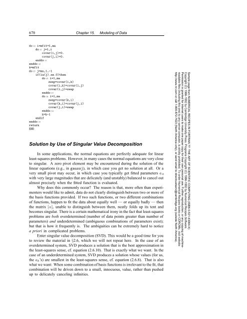
do 12 i=mfit+1,ma
do 11 j=1,i
covar(i,j)=0.
covar(j,i)=0.
enddo 11
enddo 12
k=mfit
do 15 j=ma,1,-1
if(ia(j).ne.0)then
do 13 i=1,ma
swap=covar(i,k)
covar(i,k)=covar(i,j)
covar(i,j)=swap
enddo 13
do 14 i=1,ma
swap=covar(k,i)
covar(k,i)=covar(j,i)
covar(j,i)=swap
enddo 14
k=k-1
endif
enddo 15
return
END
Solution by Use of Singular Value Decomposition
In some applications, the normal equations are perfectly adequate for linear
least-squares problems. However, in many cases the normal equations are very close
to singular. A zero pivot element may be encountered during the solution of the
linear equations (e.g., in gaussj), in which case you get no solution at all. Or a
very small pivot may occur, in which case you typically get fitted parameters a k
with very large magnitudes that are delicately (and unstably) balanced to cancel out
almost precisely when the fitted function is evaluated.
Why does this commonly occur? The reason is that, more often than experimenters
would like to admit, data do not clearly distinguish between two or more of
the basis functions provided. If two such functions, or two different combinations
of functions, happen to fit the data about equally well — or equally badly — then
the matrix [α], unable to distinguish between them, neatly folds up its tent and
becomes singular. There is a certain mathematical irony in the fact that least-squares
problems are both overdetermined (number of data points greater than number of
parameters) and underdetermined (ambiguous combinations of parameters exist);
but that is how it frequently is. The ambiguities can be extremely hard to notice
a priori in complicated problems.
Enter singular value decomposition (SVD). This would be a good time for you
to review the material in §2.6, which we will not repeat here. In the case of an
overdetermined system, SVD produces a solution that is the best approximation in
the least-squares sense, cf. equation (2.6.10). That is exactly what we want. In the
case of an underdetermined system, SVD produces a solution whose values (for us,
the ak’s) are smallest in the least-squares sense, cf. equation (2.6.8). That is also
what we want: When some combination of basis functions is irrelevant to the fit, that
combination will be driven down to a small, innocuous, value, rather than pushed
up to delicately canceling infinities.
Sample page from NUMERICAL RECIPES IN FORTRAN 77: THE ART OF SCIENTIFIC COMPUTING (ISBN 0-521-43064-X)
Copyright (C) 1986-1992 by Cambridge University Press. Programs Copyright (C) 1986-1992 by Numerical Recipes Software.
Permission is granted for internet users to make one paper copy for their own personal use. Further reproduction, or any copying of machinereadable
files (including this one) to any server computer, is strictly prohibited. To order Numerical Recipes books or CDROMs, visit website
http://www.nr.com or call 1-800-872-7423 (North America only), or send email to directcustserv@cambridge.org (outside North America).