Linear Algebra I — Martin Otto
Linear Algebra I — Martin Otto
Linear Algebra I — Martin Otto

Create successful ePaper yourself
Turn your PDF publications into a flip-book with our unique Google optimized e-Paper software.
<strong>Linear</strong> <strong>Algebra</strong> I<br />
<strong>Martin</strong> <strong>Otto</strong><br />
Winter Term 2010/11
Contents<br />
1 Introduction 5<br />
1.1 Motivating Examples . . . . . . . . . . . . . . . . . . . . . . . 5<br />
1.1.1 The two-dimensional real plane . . . . . . . . . . . . . 5<br />
1.1.2 Three-dimensional real space . . . . . . . . . . . . . . . 12<br />
1.1.3 Systems of linear equations over R n . . . . . . . . . . . 13<br />
1.1.4 <strong>Linear</strong> spaces over Z2 . . . . . . . . . . . . . . . . . . . 19<br />
1.2 Basics, Notation and Conventions . . . . . . . . . . . . . . . . 25<br />
1.2.1 Sets . . . . . . . . . . . . . . . . . . . . . . . . . . . . 25<br />
1.2.2 Functions . . . . . . . . . . . . . . . . . . . . . . . . . 27<br />
1.2.3 Relations . . . . . . . . . . . . . . . . . . . . . . . . . 32<br />
1.2.4 Summations . . . . . . . . . . . . . . . . . . . . . . . . 34<br />
1.2.5 Propositional logic . . . . . . . . . . . . . . . . . . . . 34<br />
1.2.6 Some common proof patterns . . . . . . . . . . . . . . 35<br />
1.3 <strong>Algebra</strong>ic Structures . . . . . . . . . . . . . . . . . . . . . . . 37<br />
1.3.1 Binary operations on a set . . . . . . . . . . . . . . . . 37<br />
1.3.2 Groups . . . . . . . . . . . . . . . . . . . . . . . . . . . 38<br />
1.3.3 Rings and fields . . . . . . . . . . . . . . . . . . . . . . 40<br />
1.3.4 Aside: isomorphisms of algebraic structures . . . . . . 42<br />
2 Vector Spaces 45<br />
2.1 Vector spaces over arbitrary fields . . . . . . . . . . . . . . . . 45<br />
2.1.1 The axioms . . . . . . . . . . . . . . . . . . . . . . . . 46<br />
2.1.2 Examples old and new . . . . . . . . . . . . . . . . . . 48<br />
2.2 Subspaces . . . . . . . . . . . . . . . . . . . . . . . . . . . . . 51<br />
2.2.1 <strong>Linear</strong> subspaces . . . . . . . . . . . . . . . . . . . . . 51<br />
2.2.2 Affine subspaces . . . . . . . . . . . . . . . . . . . . . . 54<br />
2.3 Aside: affine and linear spaces . . . . . . . . . . . . . . . . . . 56<br />
2.4 <strong>Linear</strong> dependence and independence . . . . . . . . . . . . . . 58<br />
3
4 <strong>Linear</strong> <strong>Algebra</strong> I <strong>—</strong> <strong>Martin</strong> <strong>Otto</strong> 2010<br />
2.4.1 <strong>Linear</strong> combinations and spans . . . . . . . . . . . . . 58<br />
2.4.2 <strong>Linear</strong> (in)dependence . . . . . . . . . . . . . . . . . . 60<br />
2.5 Bases and dimension . . . . . . . . . . . . . . . . . . . . . . . 63<br />
2.5.1 Bases . . . . . . . . . . . . . . . . . . . . . . . . . . . . 63<br />
2.5.2 Finite-dimensional vector spaces . . . . . . . . . . . . . 64<br />
2.5.3 Dimensions of linear and affine subspaces . . . . . . . . 69<br />
2.5.4 Existence of bases . . . . . . . . . . . . . . . . . . . . . 70<br />
2.6 Products, sums and quotients of spaces . . . . . . . . . . . . . 71<br />
2.6.1 Direct products . . . . . . . . . . . . . . . . . . . . . . 71<br />
2.6.2 Direct sums of subspaces . . . . . . . . . . . . . . . . . 73<br />
2.6.3 Quotient spaces . . . . . . . . . . . . . . . . . . . . . . 75<br />
3 <strong>Linear</strong> Maps 79<br />
3.1 <strong>Linear</strong> maps as homomorphisms . . . . . . . . . . . . . . . . . 79<br />
3.1.1 Images and kernels . . . . . . . . . . . . . . . . . . . . 81<br />
3.1.2 <strong>Linear</strong> maps, bases and dimensions . . . . . . . . . . . 82<br />
3.2 Vector spaces of homomorphisms . . . . . . . . . . . . . . . . 86<br />
3.2.1 <strong>Linear</strong> structure on homomorphisms . . . . . . . . . . 86<br />
3.2.2 The dual space . . . . . . . . . . . . . . . . . . . . . . 87<br />
3.3 <strong>Linear</strong> maps and matrices . . . . . . . . . . . . . . . . . . . . 89<br />
3.3.1 Matrix representation of linear maps . . . . . . . . . . 89<br />
3.3.2 Invertible homomorphisms and regular matrices . . . . 101<br />
3.3.3 Change of basis transformations . . . . . . . . . . . . . 103<br />
3.3.4 Ranks . . . . . . . . . . . . . . . . . . . . . . . . . . . 107<br />
3.4 Aside: linear and affine transformations . . . . . . . . . . . . . 112<br />
4 Matrix Arithmetic 115<br />
4.1 Determinants . . . . . . . . . . . . . . . . . . . . . . . . . . . 115<br />
4.1.1 Determinants as multi-linear forms . . . . . . . . . . . 116<br />
4.1.2 Permutations and alternating functions . . . . . . . . . 118<br />
4.1.3 Existence and uniqueness of the determinant . . . . . . 120<br />
4.1.4 Further properties of the determinant . . . . . . . . . . 124<br />
4.1.5 Computing the determinant . . . . . . . . . . . . . . . 127<br />
4.2 Inversion of matrices . . . . . . . . . . . . . . . . . . . . . . . 129<br />
4.3 Systems of linear equations revisited . . . . . . . . . . . . . . 130<br />
4.3.1 Using linear maps and matrices . . . . . . . . . . . . . 131<br />
4.3.2 Solving regular systems . . . . . . . . . . . . . . . . . . 133
Chapter 1<br />
Introduction<br />
1.1 Motivating Examples<br />
<strong>Linear</strong> algebra is concerned with the study of vector spaces. It investigates<br />
and isolates mathematical structure and methods encountered in phenomena<br />
to do with linearity. Instances of linearity arise in many different contexts<br />
of mathematics and its applications, and linear algebra provides a uniform<br />
framework for their treatment.<br />
As is typical in mathematics, the extraction of common key features that<br />
are observed in various seemingly unrelated areas gives rise to an abstraction<br />
and simplification which allows to study these crucial features in isolation.<br />
The results of this investigation can then be carried back into all those areas<br />
where the underlying common feature arises, with the benefit of a unifying<br />
perspective. <strong>Linear</strong> algebra is a very good example of a branch of mathematics<br />
motivated by the observation of structural commonality across a wide<br />
range of mathematical experience.<br />
In this rather informal introductory chapter, we consider a number of<br />
(partly very familiar) examples that may serve as a motivation for the systematic<br />
general study of “spaces with a linear structure” which is the core<br />
topic of linear algebra.<br />
1.1.1 The two-dimensional real plane<br />
The plane of basic planar geometry is modelled as R 2 = R × R, the set of<br />
ordered pairs [geordnete Paare] (x, y) of real numbers x, y ∈ R.<br />
5
6 <strong>Linear</strong> <strong>Algebra</strong> I <strong>—</strong> <strong>Martin</strong> <strong>Otto</strong> 2010<br />
<br />
p = (x, y)<br />
y •<br />
x<br />
<br />
<br />
(x, y)<br />
y<br />
<br />
<br />
v <br />
<br />
<br />
<br />
<br />
<br />
O<br />
x<br />
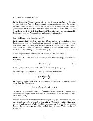
One may also think of the directed arrow pointing from the origin O =<br />
(0, 0) to the position p = (x, y) as the vector [Vektor] v = (x, y). “<strong>Linear</strong><br />
structure” in R 2 has the following features.<br />
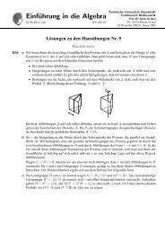
Vector addition [Vektoraddition] There is a natural addition over R 2 ,<br />
which may be introduced in two slightly different but equivalent ways.<br />
y1 + y2<br />
<br />
(x1 + x2, y1 + y2)<br />
<br />
<br />
<br />
<br />
<br />
<br />
<br />
<br />
<br />
<br />
<br />
<br />
<br />
<br />
<br />
<br />
v1<br />
+<br />
<br />
v2<br />
y2 <br />
<br />
<br />
<br />
<br />
<br />
<br />
<br />
<br />
<br />
y1 <br />
<br />
<br />
<br />
<br />
v2<br />
<br />
<br />
<br />
<br />
<br />
<br />
<br />
<br />
v1 <br />
<br />
<br />
<br />
<br />
<br />
<br />
O x2 x1 x1 + x2<br />
Arithmetically we may just lift the addition operation + R from R to R 2 ,<br />
applying it component-wise:<br />
(x, y) + R2<br />
(x ′ , y ′ ) := (x + R x ′ , y + R y ′ ).<br />
At first, we explicitly index the plus signs to distinguish their different<br />
interpretations: the new over R 2 from the old over R.<br />
Geometrically we may think of vectors v = (x, y) and v ′ = (x ′ , y ′ ) as<br />
acting as translations of the plane ; the vector v +v ′ is then the vector which<br />
corresponds to the composition of the two translations, translation through<br />
v followed by translation through v ′ . (Convince yourself that this leads to<br />
the same addition operation on R 2 .)
LA I <strong>—</strong> <strong>Martin</strong> <strong>Otto</strong> 2010 7<br />
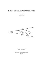
Scalar multiplication [Skalare Multiplikation] A real number r = 0 can<br />
also be used to re-scale vectors in the plane. This operation is called scalar<br />
multiplication.<br />
r · (x, y) := (r · R x, r · R y).<br />
We include scalar multiplication by r = 0, even though it maps all vectors<br />
to the null vector 0 = (0, 0) and thus does not constitute a proper re-scaling.<br />
Scalar multiplication is arithmetically induced by component-wise ordinary<br />
multiplication over R, but is not an operation over R 2 in the same sense<br />
that ordinary multiplication is an operation over R. In scalar multiplication<br />
a number (a scalar) from the number domain R operates on a vector v ∈ R 2 .<br />
<br />
(rx, ry)<br />
ry<br />
<br />
<br />
<br />
y<br />
<br />
<br />
rv<br />
<br />
<br />
<br />
<br />
<br />
<br />
<br />
<br />
<br />
<br />
<br />
<br />
<br />
v<br />
<br />
<br />
<br />
<br />
O<br />
x rx<br />
It is common practice to drop the · in multiplication notation; we shall<br />
later mostly write rv = (rx, ry) instead of r · v = (r · x, r · y).<br />
Remark There are several established conventions for vector notation; we<br />
here chose to write vectors in R2 just as pairs v = (x, y) of real numbers. 0<br />
One may equally well write the two components vertically, as in v = @x 1<br />
A.<br />
y<br />
In some contexts it may be useful to be able to switch between these<br />
two styles and explicitly refer to row vectors [Zeilenvektoren] versus column<br />
vectors [Spaltenvektoren]. Which style one adopts is largely a matter of<br />
convention – the linear algebra remains the same.<br />
Basic laws We isolate some simple arithmetical properties of vector addition<br />
and scalar multiplication; these are in fact the crucial features of what<br />
“linear structure” means, and will later be our axioms [Axiome] for vector<br />
spaces [Vektorräume]. In the following we use v, v1, . . . for arbitrary vectors<br />
(elements of R 2 in our case) and r, s for arbitrary scalars (elements of the<br />
number domain R in this case).
8 <strong>Linear</strong> <strong>Algebra</strong> I <strong>—</strong> <strong>Martin</strong> <strong>Otto</strong> 2010<br />
V1 vector addition is associative [assoziativ]. For all v1, v2, v3:<br />
(v1 + v2) + v3 = v1 + (v2 + v3).<br />
V2 vector addition has a neutral element [neutrales Element].<br />
There is a null vector 0 such that for all v:<br />
v + 0 = 0 + v = v.<br />
In R 2 , 0 = (0, 0) ∈ R 2 serves as the null vector.<br />
V3 vector addition has inverses [inverse Elemente].<br />
For every vector v there is a vector −v such that<br />
v + (−v) = (−v) + v = 0.<br />
For v = (x, y) ∈ R 2 , −v := (−x, −y) is as desired.<br />
V4 vector addition is commutative [kommutativ].<br />
For all v1, v2:<br />
v1 + v2 = v2 + v1.<br />
V5 scalar multiplication is associative.<br />
For all vectors v and scalars r, s:<br />
r · s · v = (r · s) · v.<br />
V6 scalar multiplication has a neutral element 1.<br />
For all vectors v:<br />
1 · v = v.<br />
V7 scalar multiplication is distributive [distributiv] w.r.t. the scalar.<br />
For all vectors v and all scalars r, s:<br />
(r + s) · v = r · v + s · v.<br />
V8 scalar multiplication is distributive w.r.t. the vector.<br />
For all vectors v1, v2 and all scalars r:<br />
r · <br />
v1 + v2 = r · v1 + r · v2 .
LA I <strong>—</strong> <strong>Martin</strong> <strong>Otto</strong> 2010 9<br />
All the laws in the axioms (V1-4) are immediate consequences of the corresponding<br />
properties of ordinary addition over R, since + R2 is component-wise<br />
+ R . Similarly (V5/6) are immediate from corresponding properties of multiplication<br />
over R, because of the way in which scalar multiplication between<br />
R and R2 is component-wise ordinary multiplication. Similar comments apply<br />
to the distributive laws for scalar multiplication (V7/8), but here the<br />
relationship is slightly more interesting because of the asymmetric nature of<br />
scalar multiplication.<br />
For associative operations like +, we freely write terms like a + b + c + d<br />
without parentheses, as associativity guarantees that precedence does not<br />
matter; similarly for r · s · v.<br />
Exercise 1.1.1 Annotate all + signs in the identities in (V1-8) to make clear<br />
whether they take place over R or over R 2 , and similarly mark those places<br />
where · stands for scalar multiplication and where it stands for ordinary<br />
multiplication over R.<br />
<strong>Linear</strong> equations over R2 and lines in the plane<br />
<br />
<br />
<br />
<br />
<br />
<br />
<br />
<br />
<br />
<br />
<br />
<br />
<br />
<br />
O<br />
Consider a line [Gerade] in the real plane. It can be thought of as the<br />
solution set of a linear equation [lineare Gleichung] of the form<br />
E : ax + by = c.<br />
In the equation, x and y are regarded as variables, a, b, c are fixed constants,<br />
called the coefficients of E. The solution set [Lösungsmenge] of the<br />
equation E is<br />
S(E) = {(x, y) ∈ R 2 : ax + by = c}.<br />
Exercise 1.1.2 Determine coefficients a, b, c for a linear equation E so that<br />
its solution set is the line through points p1 = (x1, y1) and p2 = (x2, y2) for<br />
two distinct given points p1 = p2 in the plane.
10 <strong>Linear</strong> <strong>Algebra</strong> I <strong>—</strong> <strong>Martin</strong> <strong>Otto</strong> 2010<br />
Looking at arbitrary linear equations of the form E, we may distinguish<br />
two degenerate cases:<br />
(i) a = b = c = 0: S(E) = R 2 is not a line but the entire plane.<br />
(ii) a = b = 0 and c = 0: S(E) = ∅ is empty (no solutions).<br />
In all other cases, S(E) really is a line. What does that mean arithmetically<br />
or algebraically, though? What can we say about the structure of the<br />
solution set in the remaining, non-degenerate cases?<br />
It is useful to analyse the solution set of an arbitrary linear equation<br />
E : ax + by = c<br />
in terms of the associated homogeneous equation<br />
E ∗ : ax + by = 0.<br />
Generally a linear equation is called homogeneous if the right-hand side is 0.<br />
Observation 1.1.1 The solution set S(E ∗ ) of any homogeneous linear equation<br />
is non-empty and closed under scalar multiplication and vector addition<br />
over R 2 :<br />
(a) 0 = (0, 0) ∈ S(E ∗ ).<br />
(b) if v ∈ S(E ∗ ), then for any r ∈ R also rv ∈ S(E ∗ ).<br />
(c) if v, v ′ ∈ S(E ∗ ), then also v + v ′ ∈ S(E ∗ ).<br />
In other words, the solution set of a homogeneous linear equation in the<br />
linear space R 2 has itself the structure of a linear space; scalar multiplication<br />
and vector addition in the surrounding space naturally restrict to the solution<br />
space and obey the same laws (V1-8) in restriction to this subspace. We shall<br />
later consider such linear subspaces systematically.<br />
Exercise 1.1.3 (i) Prove the claims of the observation.<br />
(ii) Verify that the laws (V1-8) hold in restriction to S(E ∗ ).<br />
We return to the arbitrary linear equation<br />
E : ax + by = c<br />
Observation 1.1.2 E is homogeneous (E ∗ = E) if, and only if 0 ∈ S(E).
LA I <strong>—</strong> <strong>Martin</strong> <strong>Otto</strong> 2010 11<br />
Proof. ( 1 ) Suppose first that c = 0. E : a · x + b · y = 0. Then<br />
(x, y) = 0 = (0, 0) satisfies the equation, and thus 0 ∈ S(E).<br />
Conversely, if 0 = (0, 0) ∈ S(E), then (x, y) = (0, 0) satisfies the equation<br />
E : a · x + b · y = c. Therefore a · 0 + b · 0 = c and thus c = 0 follows.<br />
✷<br />
Suppose now that E has at least one solution, S(E) = ∅. So there is<br />
some v0 ∈ S(E) [we already know that v0 = 0 if E is not homogeneous.] We<br />
claim that then the whole solution set has the form<br />
S(E) = v0 + v : v ∈ S(E ∗ ) .<br />
In other words it is the result of translating the solution set of the associated<br />
homogeneous equation through v0 where v0 is any fixed but arbitrary<br />
solution of E.<br />
Lemma 1.1.3 Consider the linear equation E : a · x + b · y = c over R 2 , with<br />
the associated homogeneous equation E ∗ : a · x + b · y = 0.<br />
(a) S(E) = ∅ if and only if c = 0 and a = b = 0.<br />
(b) Otherwise, if v0 ∈ S(E) then<br />
S(E) = v0 + v : v ∈ S(E ∗ ) .<br />
Proof. ( 1 ) (a) “If”: let a = b = 0 and c = 0. Then E is unsolvable as<br />
the left-hand side equals 0 for all x, y while the right-hand side is c = 0.<br />
“Only if”: let S(E) = ∅. Firstly, c cannot be 0, as otherwise 0 ∈ S(E) =<br />
S(E ∗ ). Similarly, if we had a = 0, then (x, y) = (c/a, 0) ∈ S(E) and if b = 0,<br />
then (x, y) = (0, c/b) ∈ S(E).<br />
(b) Let v0 = (x0, y0) ∈ S(E), so that a · x0 + b · y0 = c.<br />
We show the set equality S(E) = v0 + v : v ∈ S(E ∗ ) by showing two<br />
inclusions.<br />
S(E) ⊆ v0 + v : v ∈ S(E ∗ ) :<br />
Let v ′ = (x ′ , y ′ ) ∈ S(E). Then a · x ′ + b · y ′ = c. As also a · x0 + b · y0 = c,<br />
we have that a · x ′ + b · y ′ − (a · x0 + b · y0) = a · (x ′ − x0) + b · (y ′ − y0) = 0,<br />
whence v := (x ′ − x0, y ′ − y0) is a solution of E ∗ . Therefore v ′ = v0 + v for<br />
this v ∈ S(E ∗ ).<br />
v0 + v : v ∈ S(E ∗ ) ⊆ S(E):<br />
1 Compare section 1.2.6 for basic proof patterns encountered in these simple examples.
12 <strong>Linear</strong> <strong>Algebra</strong> I <strong>—</strong> <strong>Martin</strong> <strong>Otto</strong> 2010<br />
Let v ′ = v0 +v where v = (x, y) ∈ S(E ∗ ). Note that v ′ = (x0 +x, y0 +y).<br />
As a · x + b · y = 0 and a · x0 + b · y0 = c, we have a · (x0 + x) + b · (y0 + y) = c<br />
and therefore v ′ ∈ S(E).<br />
✷<br />
Parametric representation Let E : a·x+b·y = c be such that S(E) = ∅,<br />
and S(E) = R 2 (these are the degenerate cases). From what we saw above<br />
E is non-degenerate if and only if (a, b) = (0, 0). In this case we want to turn<br />
Lemma 1.1.3 (b) into an explicit parametric form. Put<br />
w := (−b, a). ( 2 )<br />
We check that w ∈ S(E ∗ ), and that – under the assumption that E is nondegenerate<br />
– S(E ∗ ) = {λ·w : λ ∈ R . Combining this with Lemma 1.1.3 (b),<br />
we interpret v0 ∈ S(E) as an arbitrary point on the line described by E,<br />
which in parametric form is therefore the set of points<br />
v0 + λ · w (λ ∈ R).<br />
1.1.2 Three-dimensional real space<br />
Essentially everything we did above in the two-dimensional case carries over<br />
to an analogous treatment of the n-dimensional case of R n . Because it is the<br />
second most intuitive case, and still easy to visualise, we now look at the<br />
three-dimensional case of R 3 .<br />
R 3 = R × R × R = (x, y, z): x, y, z ∈ R <br />
is the set of three-tuples (triples) of real numbers. Addition and scalar multiplication<br />
over R 3 are defined (component-wise) according to<br />
and<br />
(x1, y1, z1) + (x2, y2, z2) := (x1 + x2, y1 + y2, z1 + z2)<br />
r(x, y, z) := (rx, ry, rz),<br />
for arbitrary (x, y, z), (x1, y1, z1), (x2, y2, z2) ∈ R 3 and r ∈ R.<br />
The resulting structure on R 3 , with this addition and scalar multiplication,<br />
and null vector 0 = (0, 0, 0) satisfies the laws (axioms) (V1-8) from<br />
above. (Verify this, as an exercise!)<br />
2 Geometrically, the vector (−b, a) is orthogonal to the vector (a, b) formed by the<br />
coefficients of E ∗ .
LA I <strong>—</strong> <strong>Martin</strong> <strong>Otto</strong> 2010 13<br />
<strong>Linear</strong> equations over R 3<br />
A linear equation over R 3 takes the form<br />
E : ax + by + cz = d,<br />
for coefficients a, b, c, d ∈ R. Its solution set is<br />
S(E) = (x, y, z) ∈ R 3 : ax + by + cz = d .<br />
Again, we consider the associated homogeneous equation<br />
E ∗ : ax + by + cz = 0.<br />
In complete analogy with Observation 1.1.1 above, we find firstly that<br />
S(E ∗ ) contains 0 and is closed under vector addition and scalar multiplication<br />
(and thus is a linear subspace). Further, in analogy with Lemma 1.1.3, either<br />
S(E) = ∅ or, whenever S(E) = ∅, then<br />
S(E) = v0 + v : v ∈ S(E ∗ ) <br />
for any fixed but arbitrary solution v0 ∈ S(E).<br />
Exercise 1.1.4 Check the above claims and try to give rigorous proofs.<br />
Find out in exactly which cases E has no solution, and in exactly which cases<br />
S(E) = R 3 . Call these cases degenerate.<br />
Convince yourself, firstly in an example, that in the non-degenerate case the<br />
solution set ∅ = S(E) = R 3 geometrically corresponds to a plane within R 3 .<br />
Furthermore, this plane contains the origin (null vector 0) iff E is homogeneous.<br />
3 Can you provide a parametric representation of the set of points in<br />
such a plane?<br />
1.1.3 Systems of linear equations over R n<br />
A system of linear equations [lineares Gleichungssystem] consists of a tuple<br />
of linear equations that are to be solved simultaneously. The solution set is<br />
the intersection of the solution sets of the individual equations.<br />
A single linear equation over R n has the general form<br />
E : a1x1 + · · · + anxn = b<br />
3 “iff” is shorthand for “if, and only if”, logical equivalence or bi-implication.
14 <strong>Linear</strong> <strong>Algebra</strong> I <strong>—</strong> <strong>Martin</strong> <strong>Otto</strong> 2010<br />
with coefficients [Koeffizienten] a1, . . . , an, b ∈ R and variables [Variable,<br />
Unbestimmte] x1, . . . , xn.<br />
Considering a system of m linear equations E1, . . . , Em over R n , we index<br />
the coefficients doubly such that<br />
Ei : ai1x1 + · · · + ainxn = bi<br />
is the i-th equation with coefficients ai1, . . . , ain, bi. The entire system is<br />
⎧<br />
E :<br />
⎪⎨<br />
⎪⎩<br />
a11x1 + a12x2 + · · · + a1nxn = b1 (E1)<br />
a21x1 + a22x2 + · · · + a2nxn = b2 (E2)<br />
a31x1 + a32x2 + · · · + a3nxn = b3 (E3)<br />
am1x1 + am2x2 + · · · + amnxn = bm (Em)<br />
with m rows [Zeilen] and n columns [Spalten] on the left-hand side and one<br />
on the right-hand side. Its solution set is<br />
S(E) = v = (x1, . . . , xn) ∈ R n : v satisfies Ei for i = 1, . . . , m <br />
= S(E1) ∩ S(E2) ∩ . . . ∩ S(Em) = <br />
i=1,...,m S(Ei).<br />
The associated homogeneous system E ∗ is obtained by replacing the righthand<br />
sides (the coefficients bi) by 0.<br />
With the same arguments as in Observation 1.1.1 and Lemma 1.1.3 (b)<br />
we find the following.<br />
Lemma 1.1.4 Let E be a system of linear equations over R n .<br />
(i) The solution set of the associated homogeneous system E ∗ contains<br />
the null vector 0 ∈ R n and is closed under vector addition and scalar<br />
multiplication (and thus is a linear subspace).<br />
(ii) If S(E) = ∅ and v0 ∈ S(E) is any fixed but arbitrary solution, then<br />
S(E) = v0 + v : v ∈ S(E ∗ ) .<br />
An analogoue of Lemma 1.1.3 (a), which would tell us when the equations<br />
in E have any simultaneous solutions at all, is not so easily available at first.<br />
Consider for instance the different ways in which three planes in R 3 may<br />
intersect or fail to intersect.<br />
.
LA I <strong>—</strong> <strong>Martin</strong> <strong>Otto</strong> 2010 15<br />
Remark 1.1.5 For a slightly different perspective, consider the vectors of<br />
coefficients formed by the columns of E, ai = (a1i, a2i, . . . , ami) ∈ R m for i =<br />
1, . . . , n and b = (b1, . . . , bm) ∈ R m . Then E can be rewritten equivalently<br />
as<br />
x1a1 + x2a2 + . . . + xnan = b.<br />
(Note, incidentally, that in order to align this view with the usual layout of<br />
the system E, one might prefer to think of the ai and b as column vectors;<br />
for the mathematics of the equation, though, this makes no difference.)<br />
We shall exploit this view further in later chapters. For now we stick with<br />
the focus on rows.<br />
We now explore a well-known classical method for the effective solution<br />
of a system of linear equations. In the first step we consider individual<br />
transformations (of the schema of coefficients in E) that leave the solution<br />
set invariant. We then use these transformations systematically to find out<br />
whether E has any solutions, and if so, to find them.<br />
Row transformations<br />
If Ei : ai1x1 + . . . + ainxn = bi and Ej : aj1x1 + . . . + ajnxn = bj are rows of E<br />
and r ∈ R is a scalar, we let<br />
(i) rEi be the equation<br />
(ii) Ei + rEj be the equation<br />
rEi : (rai1)x1 + . . . + (rain)xn = rbi.<br />
Ei + rEj : (ai1 + raj1)x1 + . . . + (ain + rajn)xn = bi + rbj.<br />
Lemma 1.1.6 The following transformations on a system of linear equations<br />
leave the solution set invariant, i.e., lead from E to a new system E ′<br />
that is equivalent with E.<br />
(T1) exchanging two rows.<br />
(T2) replacing some Ei by rEi for a scalar r = 0.<br />
(T3) replacing Ei by Ei + rEj for some scalar r and some j = i.
16 <strong>Linear</strong> <strong>Algebra</strong> I <strong>—</strong> <strong>Martin</strong> <strong>Otto</strong> 2010<br />
Proof. It is obvious that (T1) does not affect S(E) as it just corresponds<br />
to a re-labelling of the equations.<br />
For (T2), it is clear that S(Ei) = S(rEi) for r = 0: for any (x1, . . . , xn)<br />
ai1x1 + . . . + ainxn = bi iff rai1x1 + . . . + rainxn = rbi.<br />
For (T3) we show for all v = (x1, . . . , xn):<br />
v ∈ S(Ei) ∩ S(Ej) iff v ∈ S(Ei + rEj) ∩ S(Ej).<br />
Assume first that v ∈ S(Ei) ∩ S(Ej).<br />
Then ai1x1 + . . . + ainxn = bi and aj1x1 + . . . + ajnxn = bj together imply<br />
that<br />
(ai1 + raj1)x1 + . . . + (ain + rajn)xn<br />
= (ai1x1 + . . . + ainxn) + r(aj1x1 + . . . + ajnxn)<br />
= bi + rbj.<br />
Therefore also v ∈ S(Ei + rEj).<br />
If, conversely, v ∈ S(Ei + rEj) ∩ S(Ej), we may appeal to the implication<br />
from left to right we just proved for arbitrary r, use it for −r in place of r<br />
and get that v ∈ S((Ei + rEj) + (−r)Ej). But (Ei + rEj) + (−r)Ej is Ei,<br />
whence v ∈ S(Ei) follows.<br />
✷<br />
Gauß-Jordan algorithm<br />
The basis of this algorithm for solving any system of linear equations is<br />
also referred to as Gaussian elimination, because it successively eliminates<br />
variables from some equations by means of the above equivalence transformations.<br />
The resulting system finally is of a form (upper triangle or echelon<br />
form [obere Dreiecksgestalt]) in which the solutions (if any) can be read off.<br />
Key step Let<br />
⎧<br />
E :<br />
⎪⎨<br />
⎪⎩<br />
a11x1 + a12x2 + · · · + a1nxn = b1 (E1)<br />
a21x1 + a22x2 + · · · + a2nxn = b2 (E2)<br />
a31x1 + a32x2 + · · · + a3nxn = b3 (E3)<br />
am1x1 + am2x2 + · · · + amnxn = bm (Em)<br />
.
LA I <strong>—</strong> <strong>Martin</strong> <strong>Otto</strong> 2010 17<br />
Assume first that a11 = 0. Then by repeated application of (T3), we may<br />
replace<br />
E2 by E2 + (−a21/a11)E1<br />
E3 by E3 + (−a31/a11)E1<br />
.<br />
Em by Em + (−am1/a11)E1<br />
with the result that the only remaining non-zero coefficient in the first column<br />
is a11:<br />
E ′ :<br />
⎧<br />
⎪⎨<br />
⎪⎩<br />
a11x1 + a12x2 + · · · + a1nxn = b1 (E1)<br />
a ′ 22x2 + · · · + a ′ 2nxn = b ′ 2 (E ′ 2)<br />
a ′ 32x2 + · · · + a ′ 3nxn = b ′ 3 (E ′ 3)<br />
a ′ m2x2 + · · · + a ′ mnxn = b ′ m (E ′ m)<br />
If a11 = 0 but some other aj1 = 0 we may apply the above steps after<br />
first exchanging E1 with Ej, according to (T1).<br />
In the remaining case that ai1 = 0 for all i, E itself already has the shape<br />
of E ′ above, even with a11 = 0.<br />
Iterated application of the key step Starting with E with m rows, we<br />
apply the key step to eliminate all coefficients in the first column in rows<br />
2, . . . , m;<br />
We then keep the first row unchanged and apply the key step again to<br />
treat the first remaining non-zero column in<br />
E ′′ :<br />
⎧<br />
⎪⎨<br />
⎪⎩<br />
a ′ 22x2 + · · · + a ′ 2nxn = b ′ 2 (E ′ 2)<br />
a ′ 32x2 + · · · + a ′ 3nxn = b ′ 3 (E ′ 3)<br />
a ′ m2x2 + · · · + a ′ mnxn = b ′ m (E ′ m)<br />
In each round we reduce the number of rows and columns still to be<br />
transformed by at least one. After at most max(m, n) rounds therefore we<br />
.<br />
.
18 <strong>Linear</strong> <strong>Algebra</strong> I <strong>—</strong> <strong>Martin</strong> <strong>Otto</strong> 2010<br />
obtain a system<br />
⎧<br />
Ê :<br />
⎪⎨<br />
⎪⎩<br />
â1j1xj1 + . . . + â1j2xj2 + . . . + â1jrxjr + . . . + â1nxn = ˆ b1<br />
â2j2xj2 + . . . + â2jrxjr + . . . + â2nxn = ˆ b2<br />
· · · · · ·<br />
ârjrxjr + . . . + ârnxn = ˆ br<br />
0 = ˆ br+1<br />
0 = ˆ br+2<br />
.<br />
0 = ˆ bm<br />
in upper triangle (echelon) form:<br />
• r is the number of rows whose left-hand sides have not been completely<br />
eliminated (note in particular that r = m can occur).<br />
• âiji = 0 is the first non-vanishing coefficient on the left-hand side in<br />
row i for i = 1, . . . , r; these coefficients are called pivot elements; the<br />
corresponding variables xjifor i = 1, . . . , r are called pivot variables.<br />
• the remaining rows r + 1, . . . , m are those whose left-hand sides have<br />
been eliminated completely.<br />
Applications of (T2) to the first r rows can further be used to make all pivot<br />
elements âiji = 1 if desired.<br />
Most importantly, S( Ê) = S(E).<br />
Reading off the solutions<br />
Lemma 1.1.7 For a system Ê in the above upper echelon form:<br />
(i) S( Ê) = ∅ unless ˆbr+1 = ˆbr+2 = . . . = ˆbm = 0.<br />
(ii) If ˆbr+1 = ˆbr+2 = . . . = ˆbm = 0, then the values for all variables that are<br />
not pivot variables can be chosen arbitrarily, and matching values for<br />
the pivot variables computed, using the i-th equation to determine xiji ,<br />
and progressing in order of i = r, r − 1, . . . , 1.<br />
Moreover, all solutions are obtained in this way.<br />
An obvious question that arises here, is whether the number of non-pivot<br />
variables that can be chosen freely in S(E) = S( Ê) depends on the particular
LA I <strong>—</strong> <strong>Martin</strong> <strong>Otto</strong> 2010 19<br />
sequence of steps in which E was transformed into upper echelon form Ê. We<br />
shall later see that this number is an invariant of the elimination procedure<br />
and related to the dimension of S(E ∗ ).<br />
1.1.4 <strong>Linear</strong> spaces over Z2<br />
We illustrate the point that scalar domains quite different from R give rise to<br />
analogous useful notions of linear structure. <strong>Linear</strong> algebra over Z2 has particular<br />
relevance in computer science – e.g., in relation to boolean functions,<br />
logic, cryptography and coding theory.<br />
Arithmetic in Z2<br />
[Compare section 1.3.2 for a more systematic account of Zn for any n, and<br />
section 1.3.3 for Zp where p is prime.]<br />
Let Z2 = {0, 1}. One may think of 0 and 1 as integers or as boolean (bit)<br />
values here; both view points will be useful.<br />
On Z2 we consider the following arithmetical operations of addition and<br />
multiplication: 4<br />
+2 0 1<br />
0 0 1<br />
1 1 0<br />
·2 0 1<br />
0 0 0<br />
1 0 1<br />
In terms of integer arithmetic, 0 and 1 and the operations +2 and ·2 may<br />
be associated with the parity of integers as follows:<br />
0 <strong>—</strong> even integers;<br />
1 <strong>—</strong> odd integers.<br />
Then +2 and ·2 describe the effect of ordinary addition and multiplication<br />
on parity. For instance, (odd) · (odd) = (odd) and (odd) + (odd) = (even).<br />
In terms of boolean values and logic, +2 is the “exclusive or” operation<br />
xor also denoted ˙∨, while ·2 is ordinary conjunction ∧.<br />
Exercise 1.1.5 Check the following arithmetical laws for (Z2, +, ·) where +<br />
is +2 and · is ·2, as declared above. We use b, b1, b2, . . . to denote arbitrary<br />
elements of Z2:<br />
4 We (at first) use subscripts in +2 and ·2 to distinguish these operations from their<br />
counterparts in ordinary arithmetic.
20 <strong>Linear</strong> <strong>Algebra</strong> I <strong>—</strong> <strong>Martin</strong> <strong>Otto</strong> 2010<br />
(i) + and · are associative and commutative.<br />
For all b1, b2, b3: (b1 + b2) + b3 = b1 + (b2 + b3);<br />
b1 + b2 = b2 + b1.<br />
Similarly for ·.<br />
(ii) · is distributive over +.<br />
For all b, b2, b3: b · (b1 + b2) = (b · b1) + (b · b2).<br />
(iii) 0 is the neutral element for +.<br />
For all b, b + 0 = 0 + b = b.<br />
1 is the neutral element for ·.<br />
For all b, b · 1 = 1 · b = b.<br />
(iv) + has inverses.<br />
For all b ∈ Z2 there is a −b ∈ Z2 such that b + (−b) = 0.<br />
(v) · has inverses for all b = 0.<br />
1 · 1 = 1 (as there is only this one instance).<br />
We now look at the space<br />
Z n 2 := (Z2) n = Z2 × · · · × Z2<br />
<br />
n times<br />
of n-tuples over Z2, or of length n bit-vectors b = (b1, . . . , bn).<br />
These can be added component-wise according to<br />
(b1, . . . , bn) + n 2 (b ′ 1, . . . , b ′ n) := (b1 +2 b ′ 1, . . . , bn +2 b ′ n). ( 5 )<br />
This addition operation provides the basis for a very simple example of<br />
a (symmetric) encryption scheme. Consider messages consisting of length n<br />
bit vectors, so that Z n 2 is our message space. Let the two parties who want<br />
to communicate messages over an insecure channel be called A for Alice and<br />
B for Bob (as is the custom in cryptography literature). Suppose Alice and<br />
Bob have agreed beforehand on some bit-vector k = (k1, . . . , kn) ∈ Z n 2 to be<br />
their shared key, which they keep secret from the rest of the world.<br />
If Alice wants to communicate message m = (m1, . . . , mn) ∈ Z n 2 to Bob,<br />
she sends the encrypted message<br />
m ′ := m + k<br />
5 Again, the distinguishing markers for the different operations of addition will soon be<br />
dropped.
LA I <strong>—</strong> <strong>Martin</strong> <strong>Otto</strong> 2010 21<br />
and Bob decrypts the bit-vector m ′ that he receives, according to<br />
m ′′ := m ′ + k<br />
using the same key k. Indeed, the arithmetic of Z2 and Z n 2 guarantees that<br />
always m ′′ = m. This is a simple consequence of the peculiar feature that<br />
b + b = 0 for all b ∈ Z2, (addition in Z2)<br />
whence also b + b = 0 for all b ∈ Z n 2. (addition in Z n 2)<br />
Cracking this encryption is just as hard as to come into possession of the<br />
agreed key k – considered sufficiently unlikely in the short run if its length<br />
n is large and if there are no other regularities to go by (!). Note that the<br />
key is actually retrievable from any pair of plain and encrypted messages<br />
k = m + m ′ .<br />
Example, for n = 8 and with k = (0, 0, 1, 0, 1, 1, 0, 1); remember that<br />
addition in Z n 2 is bit-wise ˙∨ (exclusive or):<br />
m = 10010011<br />
k = 00101101<br />
m ′ = m + k = 10111110<br />
and m ′ = 10111110<br />
k = 00101101<br />
m = m ′ + k = 10010011<br />
We also define scalar multiplication over Z n 2, between b = (b1, . . . , bn) ∈<br />
Z n 2 and λ ∈ Z2:<br />
λ · (b1, . . . , bn) := (λ · b1, . . . , λ · bn).<br />
Exercise 1.1.6 Verify that Z n 2 with vector addition and scalar multiplication<br />
as introduced above satisfies all the laws (V1-8) (with null vector<br />
0 = (0, . . . , 0)).<br />
Parity check-bit<br />
This is a basic example from coding theory. The underlying idea is used<br />
widely, for instance in supermarket bar-codes or in ISBN numbers. Consider<br />
bit-vectors of length n, i.e., elements of Z n 2. Instead of using all possible<br />
bit-vectors in Z n 2 as carriers of information, we restrict ourselves to some<br />
subspace C ⊆ Z n 2 of admissible codes. The possible advantage of this is that<br />
small errors (corruption of a few bits in one of the admissible vectors) may
22 <strong>Linear</strong> <strong>Algebra</strong> I <strong>—</strong> <strong>Martin</strong> <strong>Otto</strong> 2010<br />
become easily detectable, or even repairable – the fundamental idea in error<br />
detecting and error correcting codes. <strong>Linear</strong> algebra can be used to devise<br />
such codes and to derive efficient algorithms for dealing with them. This is<br />
particularly so for linear codes C ⊆ Z n 2, whose distinguishing feature is their<br />
closure under addition in Z n 2.<br />
The following code with parity check-bit provides the most fundamental<br />
example, of a (weak) error-detecting code. Let n > 2 and consider the<br />
following linear equation over Z n 2:<br />
with solution set<br />
E+ : x1 + · · · + xn−1 + xn = 0<br />
C+ = S(E+) = (b1, . . . , bn) ∈ Z n 2 : b1 + · · · + bn−1 + bn = 0 .<br />
Note that the linear equation E+ has coefficients over Z2, namely just 1s<br />
on the left hand side, and 0 on the right (hence homogeneous), and is based<br />
on addition in Z2. A bit-vector satisfies E+ iff its parity sum is even, i.e., iff<br />
the number of 1s is even.<br />
Exercise 1.1.7 How many bit-vectors are there in Z n 2? What is the proportion<br />
of bit-vectors in C+?<br />
Check that C+ ⊆ Z n 2 contains the null vector and is closed under vector<br />
addition in Z n 2 (as well as under scalar multiplication). It thus provides an<br />
example of a linear subspace, and hence a so-called linear code.<br />
Suppose that some information (like that on an identification tag for<br />
goods) is coded using not arbitrary bit-vectors in Z n 2 but just bit-vectors from<br />
the subspace C+. Suppose further that some non-perfect data-transmission<br />
(e.g. through a scanner) results in some errors but that one can mostly rely on<br />
the fact that at most one bit gets corrupted. In this case a test whether the<br />
resulting bit-vector (as transmitted by the scanner say) still satisfies E+ can<br />
reliably tell whether an error has occurred or not. This is because whenever<br />
v = (b1, . . . , bn) and v ′ = (b ′ 1, . . . , b ′ n) differ in precisely one bit, then v ∈ C+<br />
iff v ′ ∈ C+.<br />
From error-detecting to error-correcting<br />
Better (and sparser) codes C ⊆ Z n 2 can be devised which allow not just to<br />
detect but even to repair corruptions that only affect a small number of bits.
LA I <strong>—</strong> <strong>Martin</strong> <strong>Otto</strong> 2010 23<br />
If C ⊆ Z n 2 is such that any two distinct elements v, v ′ ∈ C differ in at least<br />
2t + 1 bits for some constant t, then C provides a t-error-correcting code.<br />
If ˆv is a possibly corrupted version of v ∈ C but differs from v in at most<br />
t places, then v is uniquely determined as the unique element of C which<br />
differs from ˆv in at most t places. In case of linear codes C, linear algebra<br />
provides techniques for efficient error-correction procedures in this setting.<br />
Boolean functions in two variables<br />
This is another example of spaces Z n 2 in the context of boolean algebra and<br />
propositional logic. Consider the set B 2 of all boolean functions in two variables<br />
(which we here denote r and s)<br />
f : Z2 × Z2 −→ Z2<br />
(r, s) ↦−→ f(r, s)<br />
Each such f ∈ B 2 is fully represented by its table of values<br />
r s f(r, s)<br />
0 0 f(0, 0)<br />
0 1 f(0, 1)<br />
1 0 f(1, 0)<br />
1 1 f(1, 1)<br />
or more succinctly by just the 4-bit vector<br />
f := (f(0, 0), f(0, 1), f(1, 0), f(1, 1)) ∈ Z 4 2.<br />
We have for instance the following correspondences:<br />
function f ∈ B 2 arithmetical description of f vector f ∈ Z 4 2<br />
constant 0 (r, s) ↦→ 0 (0, 0, 0, 0)<br />
constant 1 (r, s) ↦→ 1 (1, 1, 1, 1)<br />
projection r (r, s) ↦→ r (0, 0, 1, 1)<br />
projection s (r, s) ↦→ s (0, 1, 0, 1)<br />
negation of r, ¬r (r, s) ↦→ 1 − r (1, 1, 0, 0)<br />
negation of s, ¬s (r, s) ↦→ 1 − s (1, 0, 1, 0)<br />
exclusive or, ˙∨ (xor) (r, s) ↦→ r +2 s (0, 1, 1, 0)<br />
conjunction, ∧ (r, s) ↦→ r ·2 s (0, 0, 0, 1)<br />
Sheffer stroke, | (nand) (r, s) ↦→ 1 − r ·2 s (1, 1, 1, 0)
24 <strong>Linear</strong> <strong>Algebra</strong> I <strong>—</strong> <strong>Martin</strong> <strong>Otto</strong> 2010<br />
The map<br />
: B 2 −→ Z 4 2<br />
f ↦−→ f<br />
is a bijection. In other words, it establishes a one-to-one and onto correspondence<br />
between the sets B 2 and Z 4 2. Compare section 1.2.2 on (one-to-one)<br />
functions and related notions. (In fact more structure is preserved in this<br />
case; more on this later.)<br />
It is an interesting fact that all functions in B 2 can be expressed in terms<br />
of compositions of just r, s and |. 6 For instance, ¬r = r|r, 1 = (r|r)|r, and<br />
r ∧ s = (r|s)|(r|s). Consider the following questions:<br />
Is this is also true with ˙∨ (exclusive or) instead of Sheffer’s |?<br />
If not, can all functions in B 2 be expressed in terms of 0, 1, r, s, ˙∨, ¬?<br />
If not all, which functions in B 2 do we get?<br />
Lemma 1.1.8 Let f1, f2 ∈ B 2 be represented by f 1 , f 2 ∈ Z 4 2. Then the<br />
function<br />
f1 ˙∨f2 : (r, s) ↦−→ f1(r, s) ˙∨f2(r, s)<br />
is represented by<br />
f1 ˙∨f2 = f 1 + f 2 . (vector addition in Z 4 2)<br />
Proof. By agreement of ˙∨ with +2. For all r, s:<br />
(f1 ˙∨f2)(r, s) = f1(r, s) ˙∨f2(r, s) = f1(r, s) +2 f2(r, s).<br />
Corollary 1.1.9 The boolean functions f ∈ B 2 that are generated from<br />
r, s, ˙∨ all satisfy<br />
f ∈ C+ = S(E+) = f : f(0, 0) + f(0, 1) + f(1, 0) + f(1, 1) = 0 .<br />
Here E+ : x1 + x2 + x3 + x4 = 0 is the same homogeneous linear equation<br />
considered for the parity check bit above.<br />
Conjunction r ∧ s, for instance, cannot be generated from r, s, ˙∨.<br />
6 This set of functions is therefore said to be expressively complete; so are for instance<br />
also r, s with negation and conjunction.<br />
✷
LA I <strong>—</strong> <strong>Martin</strong> <strong>Otto</strong> 2010 25<br />
Proof. We show that all functions that can be generated from r, s, ˙∨<br />
satisfy the condition by showing the following:<br />
(i) the basic functions r and s satisfy the condition;<br />
(ii) if some functions f1 and f2 satisfy the condition then so does f1 ˙∨f2.<br />
This implies that no functions generated from r, s, ˙∨ can break the condition<br />
– what we want to show. 7<br />
Check (i): r = (0, 0, 1, 1) ∈ C+; s = (0, 1, 0, 1) ∈ C+.<br />
(ii) follows from Lemma 1.1.8 as C+ is closed under + 4 2, being the solution<br />
set of a homogeneous linear equation (compare Exercise 1.1.7).<br />
For the assertion about conjunction, observe that ∧ = (0, 0, 0, 1) ∈ C+.<br />
✷<br />
Exercise 1.1.8 Show that the functions generated by r, s, ˙∨ do not even<br />
cover all of C+ but only a smaller subspace of Z 4 2. Find a second linear<br />
equation over Z 4 2 that together with E+ precisely characterises those f which<br />
are generated from r, s, ˙∨.<br />
Exercise 1.1.9 The subset of B 2 generated from r, s, 0, 1, ˙∨, ¬ (allowing the<br />
constant functions and negation as well) is still strictly contained in B 2 ;<br />
conjunction is still not expressible. In fact the set of functions thus generated<br />
precisely corresponds to the subspace associated with C+ ⊆ Z 4 2.<br />
1.2 Basics, Notation and Conventions<br />
Note: This section is intended as a glossary of terms and basic concepts to<br />
turn to as they arise in context; and not so much to be read in one go.<br />
1.2.1 Sets<br />
Sets [Mengen] are unstructured collections of objects (the elements [Elemente]<br />
of the set) without repetitions. In the simplest case a set is denoted<br />
by an enumeration of its elements, inside set brackets. For instance, {0, 1}<br />
denotes the set whose only two elements are 0 and 1.<br />
7 This is a proof by a variant of the principle of proof by induction which works not<br />
just over N. Compare section 1.2.6.
26 <strong>Linear</strong> <strong>Algebra</strong> I <strong>—</strong> <strong>Martin</strong> <strong>Otto</strong> 2010<br />
Some important standards sets:<br />
N = {0, 1, 2, 3, . . .} the set of natural numbers 8 [natürliche Zahlen]<br />
Z the set of integers [ganze Zahlen]<br />
Q the set of rationals [rationale Zahlen]<br />
R the set of reals [relle Zahlen]<br />
C the set of complex numbers [komplexe Zahlen]<br />
Membership, set inclusion, set equality, power set<br />
For a set A: a ∈ A (a is an element of A). a ∈ A is an abbreviation for “not<br />
a ∈ A”, just as a = b is shorthand for “not a = b”.<br />
∅ denotes the empty set [leere Menge], so that a ∈ ∅ for any a.<br />
B ⊆ A (B is a subset [Teilmenge] of A) if for all a ∈ B we have a ∈ A. For<br />
instance, ∅ ⊆ {0, 1} ⊆ N ⊆ Z ⊆ Q ⊆ R ⊆ C. The power set [Potenzmenge]<br />
of a set A is the set of all subsets of A, denoted P(A).<br />
Two sets are equal, A1 = A2, if and only if they have precisely the same<br />
elements (for all a: a ∈ A1 if and only if a ∈ A2). This is known as the<br />
principle of extensionality [Extensionalität].<br />
It is often useful to test for equality via: A1 = A2 if and only if both<br />
A1 ⊆ A2 and A2 ⊆ A1.<br />
The strict subset relation A B says that A ⊆ B and A = B, equivalently:<br />
A ⊆ B and not B ⊆ A. ( 9 )<br />
Set operations: intersection, union, difference, and products<br />
The following are the most common (boolean) operations on sets.<br />
Intersection [Durchschnitt] of sets, A1 ∩ A2. The elements of A1 ∩ A2 are<br />
precisely those that are elements of both A1 and A2.<br />
Union [Vereinigung] of sets , A1∪A2. The elements of A1∪A2 are precisely<br />
those that are elements of at least one of A1 or A2.<br />
Set difference [Differenz], A1 \ A2, is defined to consist of precisely those<br />
a ∈ A1 that are not elements of A2.<br />
8 Note that we regard 0 as a natural number; there is a competing convention according<br />
to which it is not. It does not really matter but one has to be aware of the convention<br />
that is in effect.<br />
9 The subset symbol without the horizontal line below is often used in place of our ⊆,<br />
but occasionally also to denote the strict subset relation. We here try to avoid it.
LA I <strong>—</strong> <strong>Martin</strong> <strong>Otto</strong> 2010 27<br />
Cartesian products and tuples<br />
Cartesian products provide sets of tuples. The simplest case of tuples is that<br />
of (ordered) pairs [(geordnete) Paare]. (a, b) is the ordered pair whose first<br />
component is a and whose second component is b. Two ordered pairs are<br />
equal iff they agree in both components:<br />
(a, b) = (a ′ , b ′ ) iff a = a ′ and b = b ′ .<br />
One similarly defines n-tuples [n-Tupel] (a1, . . . , an) with n components<br />
for any n 2. For some small n these have special names, namely pairs<br />
(n = 2), triples (n = 3), etc.<br />
The cartesian product [Kreuzprodukt] of two sets, A1 × A2, is the set of<br />
all ordered pairs (a1, a2) with a1 ∈ A1 and a2 ∈ A2.<br />
Multiple cartesian products A1 × A2 × · · · × An are similarly defined. The<br />
elements of A1 × A2 × · · · × An are the n-tuples whose i-th components are<br />
elements of Ai, for i = 1, . . . , n.<br />
In the special case that the cartesian product is built from the same set<br />
A for all its components, one writes An for the set of n-tuples over A instead<br />
of A<br />
<br />
× A ×<br />
<br />
· · · × A<br />
<br />
.<br />
n times<br />
Defined subsets New sets are often defined as subsets of given sets. If p<br />
states a property that elements a ∈ A may or may not have, then B = {a ∈<br />
A: p(a)} denotes the subset of A that consists of precisely those elements of<br />
A that do have property p. For instance, {n ∈ N: 2 divides n} is the set of<br />
even natural numbers, or {(x, y) ∈ R 2 : ax + by = c} is the solution set of the<br />
linear equation E : ax + by = c.<br />
1.2.2 Functions<br />
Functions [Funktionen] (or maps [Abbildungen]) are the next most fundamental<br />
objects of mathematics after sets. Intuitively a function maps elements<br />
of one set (the domain [Definitionsbereich] of the function) to elements<br />
of another set (the range [Wertebereich] of the function). A function f thus<br />
prescribes for every element a of its domain precisely one element f(a) in the<br />
range. The full specification of a function f therefore has three parts:<br />
(i) the domain, a set A = dom(f),<br />
(ii) the range, a set B = range(f),
28 <strong>Linear</strong> <strong>Algebra</strong> I <strong>—</strong> <strong>Martin</strong> <strong>Otto</strong> 2010<br />
(iii) the association of precisely one f(a) ∈ B with every a ∈ A.<br />
Standard notation is as in<br />
f : A −→ B<br />
a ↦−→ f(a)<br />
where the first line specifies sets A and B as domain and range, respectively,<br />
and the second line specifies the mapping prescription for all a ∈ A. For<br />
instance, f(a) may be given as an arithmetical term. Any other description<br />
that uniquely determines an element f(a) ∈ B for every a ∈ A is admissible.<br />
a<br />
•<br />
•<br />
<br />
A<br />
<br />
B<br />
•<br />
a •<br />
′<br />
f(a)<br />
f(a ′ <br />
<br />
<br />
)<br />
Examples<br />
f(a) is the image of a under f [Bild];<br />
a is a pre-image of b = f(a) [Urbild].<br />
idA : A −→ A identity function on A<br />
a ↦−→ a<br />
succ: N −→ N successor function on N<br />
n ↦−→ n + 1<br />
+: N × N −→ N natural number addition ( 10 )<br />
(n, m) ↦−→ n + m<br />
prime: N −→ {0, 1}<br />
n ↦−→<br />
<br />
1<br />
0<br />
if n is prime<br />
else<br />
characteristic function<br />
of the set of primes<br />
f(a1,...,an) : R n −→ R a linear function<br />
(x1, . . . , xn) ↦−→ a1x1 + · · · + anxn
LA I <strong>—</strong> <strong>Martin</strong> <strong>Otto</strong> 2010 29<br />
With a function f : A → B we associate its image set [Bildmenge]<br />
image(f) = f(a): a ∈ A ⊆ B,<br />
consisting of all the images of elements of A under f.<br />
The actual association between a ∈ dom(f) and f(a) ∈ range(f) prescribed<br />
in f is often best visualised in term of the set of all pre-image/image<br />
pairs, called the graph [Graph] of f:<br />
Gf = (a, f(a)): a ∈ A ⊆ A × B.<br />
Exercise 1.2.1 Which properties must a subset G ⊆ A × B have in order<br />
to be the graph of some function f : A → B?<br />
Surjections, injections, bijections<br />
<br />
f(x) •(x,<br />
f(x))<br />
Definition 1.2.1 A function f : A → B is said to be<br />
(i) surjective (onto) if image(f) = B,<br />
(ii) injective (one-to-one) if for all a, a ′ ∈ A: f(a) = f(a ′ ) ⇒ a = a ′ ,<br />
(iii) bijective if it is injective and surjective.<br />
Correspondingly, the function f is called a surjection [Surjektion], an<br />
injection [Injektion], or a bijection [Bijektion], respectively.<br />
Exercise 1.2.2 Classify the above example functions in these terms.<br />
10 Functions that are treated as binary operations like +, are sometimes more naturally<br />
written with the function symbol between the arguments, as in n+m rather than +(n, m),<br />
but the difference is purely cosmetic.<br />
x
30 <strong>Linear</strong> <strong>Algebra</strong> I <strong>—</strong> <strong>Martin</strong> <strong>Otto</strong> 2010<br />
Note that injectivity of f means that every b ∈ range(f) has at most one<br />
pre-image; surjectivity says that it has at least one, and bijectivity says that<br />
it has precisely one pre-image.<br />
Bijective functions f : A → B play a special role as they precisely translate<br />
one set into another at the element level. In particular, the existence<br />
of a bijection f : A → B means that A and B have the same size. [This is<br />
the basis of the set theoretic notion of cardinality of sets, applicable also for<br />
infinite sets.]<br />
If f : A → B is bijective, then the following is a well-defined function<br />
f −1 : B −→ A<br />
b ↦−→ the a ∈ A with f(a) = b.<br />
f −1 is called the inverse function of f [Umkehrfunktion].<br />
Composition<br />
If f : A → B and g : B → C are functions, we may define their composition<br />
g ◦ f : A −→ C<br />
a ↦−→ g(f(a))<br />
We read “g ◦ f” as “g after f”.<br />
Note that in the case of the inverse f −1 of a bijection f : A → B, we have<br />
f −1 ◦ f = idA and f ◦ f −1 = idB.<br />
Exercise 1.2.3 Find examples of functions f : A → B that have no inverse<br />
(because they are not bijective) but admit some g : B → A such that either<br />
g ◦ f = idA or f ◦ g = idB.<br />
How are these conditions related to injectivity/surjectivity of f?<br />
Permutations<br />
A permutation [Permutation] is a bijective function of the form f : A → A.<br />
Their action on the set A may be viewed as a re-shuffling of the elements,<br />
hence the name permutation. Because they are bijective (and hence invertible)<br />
and lead from A back into A they have particularly nice composition<br />
properties.
LA I <strong>—</strong> <strong>Martin</strong> <strong>Otto</strong> 2010 31<br />
In fact the set of all permutations of a fixed set A, together with the<br />
composition operation ◦ forms a group, which means that it satisfies the<br />
laws (G1-3) collected below (compare (V1-3) above and section 1.3.2).<br />
For a set A, let Sym(A) be the set of permutations of A<br />
Sym(A) = f : f a bijection from A to A ,<br />
equipped with the composition operation<br />
◦: Sym(A) × Sym(A) −→ Sym(A)<br />
(f1, f2) ↦−→ f1 ◦ f2.<br />
Exercise 1.2.4 Check that (Sym(A), ◦, idA) satisfies the following laws:<br />
G1 (associativity)<br />
For all f, g, h ∈ Sym(A):<br />
f ◦ g ◦ h = f ◦ g ◦ h.<br />
G2 (neutral element)<br />
idA is a neutral element w.r.t. ◦, i.e., for all f ∈ Sym(A):<br />
f ◦ idA = idA ◦ f = f.<br />
G3 (inverse elements)<br />
For every f ∈ Sym(A) there is an f ′ ∈ Sym(A) such that<br />
f ◦ f ′ = f ′ ◦ f = idA.<br />
Give an example to show that ◦ is not commutative.<br />
Definition 1.2.2 For n 1, Sn := (Sym({1, . . . , n}), ◦, id{1,...,n}), the group<br />
of all permutations of an n element set, with composition, is called the symmetric<br />
group [symmetrische Gruppe] of n elements.<br />
Common notation for f ∈ Sn is f =<br />
1<br />
f(1)<br />
2<br />
f(2)<br />
· · ·<br />
n<br />
f(n)<br />
Exercise 1.2.5 What is the size of Sn, i.e., how many different permutations<br />
does a set of n elements have?<br />
List all the elements of S3 and compile the table of the operation ◦ over S3.<br />
<br />
.
32 <strong>Linear</strong> <strong>Algebra</strong> I <strong>—</strong> <strong>Martin</strong> <strong>Otto</strong> 2010<br />
1.2.3 Relations<br />
An r-ary relation [Relation] R over a set A is a collection of r-tuples (a1, . . . , ar)<br />
over A, i.e., a subset R ⊆ A r . For binary relations R ⊆ A 2 one often uses<br />
notation aRa ′ instead of (a, a ′ ) ∈ R.<br />
For instance, the natural order relation < is a binary relation over N<br />
consisting of all pairs (n, m) with n < m.<br />
The graph of a function f : A → A is a binary relation.<br />
One may similarly consider relations across different sets, as in R ⊆ A×B;<br />
for instance the graph of a function f : A → B is a relation in this sense.<br />
Equivalence relations<br />
These are a particularly important class of binary relations. A binary relation<br />
R ⊆ A2 is an equivalence relation [ Äquivalenzrelation] over A iff it is<br />
(i) reflexive [reflexiv]; for all a ∈ A, (a, a) ∈ R.<br />
(ii) symmetric [symmetrisch]; for all a, b ∈ A: (a, b) ∈ R iff (b, a) ∈ R.<br />
(iii) transitive [transitiv]; for all a, b, c ∈ A: if (a, b) ∈ R and (b, c) ∈ R,<br />
then (a, c) ∈ R.<br />
Examples: equality (over any set); having the same parity (odd or even)<br />
over Z; being divisible by exactly the same primes, over N.<br />
Non-examples: on N; having absolute difference less than 5 over N.<br />
Exercise 1.2.6 Let f : A → B be a function. Show that the following is an<br />
equivalence relation:<br />
Rf := (a, a ′ ) ∈ A 2 : f(a) = f(a ′ ) .<br />
Exercise 1.2.7 Consider the following relationship between arbitrary sets<br />
A, B: A ∼ B if there exists some bijection f : A → B. Show that this<br />
relationship has the properties of an equivalence relation: ∼ is reflexive,<br />
symmetric and transitive.<br />
Any equivalence relation over a set A partitions A into equivalence classes.<br />
Let R be an equivalence relation over A. The R-equivalence class of a ∈ A<br />
is the subset<br />
[a]R = a ′ : (a, a ′ ) ∈ R .
LA I <strong>—</strong> <strong>Martin</strong> <strong>Otto</strong> 2010 33<br />
Exercise 1.2.8 Show that for any two equivalence classes [a]R and [a ′ ]R,<br />
either [a]R = [a ′ ]R or [a]R ∩ [a ′ ]R = ∅, and that A is the disjoint union of its<br />
equivalence classes w.r.t. R.<br />
The set of equivalence classes is called the quotient of the underlying set<br />
A w.r.t. the equivalence relation R, denoted A/R:<br />
A/R = [a]R : a ∈ A .<br />
The function πR : A → A/R that maps each element a ∈ A to its equivalence<br />
class [a]R ∈ A/R is called the natural projection. Note that (a, a ′ ) ∈ R<br />
iff [a]R = [a ′ ]R iff πR(a) = πR(a ′ ). Compare the diagram for an example of an<br />
equivalence relation with 3 classes that are represented, e.g., by the pairwise<br />
inequivalent elements a, b, c ∈ A:<br />
A<br />
A/R<br />
a<br />
<br />
<br />
<br />
<br />
<br />
<br />
<br />
<br />
<br />
<br />
<br />
<br />
<br />
<br />
<br />
<br />
<br />
<br />
<br />
<br />
•<br />
[a]R<br />
<br />
<br />
<br />
<br />
<br />
<br />
<br />
<br />
<br />
<br />
<br />
<br />
<br />
<br />
b <br />
<br />
<br />
<br />
<br />
<br />
<br />
<br />
c<br />
•<br />
[b]R<br />
•<br />
[c]R<br />
<br />
<br />
<br />
<br />
<br />
<br />
<br />
<br />
<br />
<br />
<br />
<br />
<br />
<br />
<br />
For the following also compare section 1.3.2.<br />
Exercise 1.2.9 Consider the equivalence relation ≡n on Z defined as<br />
a ≡n b iff a = kn + b for some k ∈ Z.<br />
Integers a and b are equivalent in this sense if their difference is divisible by<br />
n, or if they leave the same remainder w.r.t. division by n.<br />
Check that ≡n is an equivalence relation over Z, and that every equivalence<br />
class has a unique member in Zn = {0, . . . , n − 1}.<br />
Show that addition and multiplication in Z operate class-wise, in the<br />
sense that for all a ≡n a ′ and b ≡n b ′ we also have a + b ≡n a ′ + b ′ and<br />
ab ≡n a ′ b ′ .
34 <strong>Linear</strong> <strong>Algebra</strong> I <strong>—</strong> <strong>Martin</strong> <strong>Otto</strong> 2010<br />
1.2.4 Summations<br />
As we deal with (vector and scalar) sums a lot, it is useful to adopt the usual<br />
concise summation notation. We write for instance<br />
n<br />
aixi for a1x1 + · · · + anxn.<br />
i=1<br />
Relaxed variants of the general form <br />
i∈I ai where I is some index set<br />
that indexes a family (ai)i∈I of terms to be summed up are useful. (In our<br />
usage of such notation, I has to be finite or at least only finitely many ai = 0.)<br />
This convention implicitly appeals to associativity and commutativity of the<br />
underlying addition operation (why?).<br />
Similar conventions apply to other associative and commutative operations,<br />
in particular set union and intersection (and here finiteness of the index<br />
set is not essential). For instance <br />
i∈I Ai stands for the union of all the sets<br />
Ai for i ∈ I.<br />
1.2.5 Propositional logic<br />
We here think of propositions as assertions [Aussagen] about mathematical<br />
objects, and are mostly interested in (determining) their truth or falsity.<br />
Typically propositions are structured, and composed from simpler propositions<br />
according to certain logical composition operators. Propositional logic<br />
[Aussagenlogik], and the standardised use of the propositional connectives<br />
comprising negation, conjunction and disjunction, plays an important role in<br />
mathematical arguments.<br />
If A is an assertion then ¬A (not A [nicht A]) stands for the negation<br />
[Negation] of A and is true exactly when A itself is false and vice versa.<br />
For assertions A and B, A ∧ B (A and B [A und B]) stands for their<br />
conjuction [Konjunktion], which is true precisely when both A and B are<br />
true.<br />
A ∨ B (A or B [A oder B]) stands for their disjunction [Disjunktion],<br />
which is true precisely when at least one of A and B is true.<br />
The standardised semantics of these basic logical operators, and other<br />
derived ones, can be described in terms of truth tables. Using the boolean<br />
values 0 and 1 as truth values, 0 for false and 1 for true, the truth table for a
LA I <strong>—</strong> <strong>Martin</strong> <strong>Otto</strong> 2010 35<br />
logical operator specifies the truth value of the resulting proposition in terms<br />
of the truth values for the component propositions. 11<br />
A B ¬A A ∧ B A ∨ B A ⇒ B A ⇔ B<br />
0 0 1 0 0 1 1<br />
0 1 1 0 1 1 0<br />
1 0 0 0 1 0 0<br />
1 1 0 1 1 1 1<br />
The implication [Implikation] A ⇒ B (A implies B [A impliziert B] is<br />
true unless A (the premise or assumption) is true and B (the conclusion) is<br />
false. The truth table therefore is the same as for ¬A ∨ B.<br />
The equivalence or bi-implication [ Äquivalenz], A ⇔ B (A is equivalent<br />
[äquivalent] with B, A if and and only if B [A genau dann wenn B]), is true<br />
precisely if A and B have the same truth value.<br />
It is common usage to write and read a bi-implication as A iff B, where<br />
“iff” abbreviates “if and only if” [gdw: genau dann wenn].<br />
We do not give any formal account of quantification, and only treat the<br />
symbolic quantifiers ∀ and ∃ as occasional shorthand notation for “for all”<br />
and “there exists”, as in ∀x, y ∈ R (x + y = y + x).<br />
1.2.6 Some common proof patterns<br />
Implications It is important to keep in mind that an implication A ⇒ B<br />
is proved if we establish that B must hold whenever A is true (think of A as<br />
the assumption, of B as the conclusion claimed under this assumption). No<br />
claim at all is made about settings in which (the assumption) A fails!<br />
To prove an implication A ⇒ B, one can either assume A and establish<br />
B, or equivalently assume ¬B (the negation of B) and work towards ¬A; the<br />
justification of the latter lies in the fact that A ⇒ B is logically equivalent<br />
with its contraposition [Kontraposition] ¬B ⇒ ¬A (check the truth tables.)<br />
11 Note that these precise formal conventions capture some aspects of the natural everyday<br />
usage of “and” and “or”, or “if . . . , then . . . ”, but not all. In particular, the truth<br />
or falsehood of a natural language composition may depend not just on the truth values<br />
of the component assertions but also on context. The standardised interpretation may<br />
therefore differ from your intuitive understanding at least in certain contexts.
36 <strong>Linear</strong> <strong>Algebra</strong> I <strong>—</strong> <strong>Martin</strong> <strong>Otto</strong> 2010<br />
Implications often occur as chains of the form<br />
A ⇒ A1, A1 ⇒ A2, A2 ⇒ A3, . . . , An ⇒ B,<br />
or A ⇒ A1 ⇒ A2 ⇒ . . . ⇒ B for short. The validity of (each step in) the<br />
chain then also implies the validity of A ⇒ B. Indeed, one often constructs<br />
a chain of intermediate steps in the course of a proof of A ⇒ B.<br />
Indirect proof In order to prove A, it is sometimes easier to work indirectly,<br />
by showing that ¬A leads to a contradiction. Then, as ¬A is seen to<br />
be an impossibility, A must be true.<br />
Bi-implications or equivalences To establish an equivalence A ⇔ B one<br />
often shows separately A ⇒ B and B ⇒ A. Chains of equivalences of the<br />
form<br />
A ⇔ A1, A1 ⇔ A2, A2 ⇔ . . . ⇔ B,<br />
or A ⇔ A1 ⇔ A2 ⇔ . . . ⇔ B for short, may allow us to establish A ⇔ B<br />
through intermediate steps. Another useful trick for establishing an equivalence<br />
between several assertions, say A, B and C for instance, is to prove a<br />
circular chain of one-sided implications, for instance<br />
A ⇒ C ⇒ B ⇒ A<br />
that involves all the assertions in some order that facilitates the proof.<br />
Induction [vollständige Induktion] Proofs by induction are most often used<br />
for assertions A(n) parametrised by the natural numbers n ∈ N. In order to<br />
show that A(n) is true for all n ∈ N one establishes<br />
(i) the truth of A(0) (the base case),<br />
(ii) the validity of the implication A(n) ⇒ A(n+1) in general, for all n ∈ N<br />
(the induction step).<br />
As any individual natural number m is reached from the first natural<br />
number 0 in finitely many successor steps from n to n+1, A(m) is established<br />
in this way via a chain of implications that takes us from the base case A(0)<br />
to A(m) via a number of applications of the induction step.<br />
That the natural numbers support the principle of induction is axiomatically<br />
captured in Peano’s induction axiom; this is the axiomatic counterpart<br />
of the intuitive insight just indicated.
LA I <strong>—</strong> <strong>Martin</strong> <strong>Otto</strong> 2010 37<br />
There are many variations of the technique. In particular, in order to<br />
prove A(n + 1) one may assume not just A(n) but all the previous instances<br />
A(0), . . . , A(n) without violating the validity of the principle.<br />
But also beyond the domain of natural numbers similar proof principles<br />
can be used, whenever the domain in question can similarly be generated<br />
from some basic instances via some basic construction steps (“inductive data<br />
types”). If A is true of the basic instances, and the truth of A is preserved<br />
in each construction step, then A must be true of all the objects that can be<br />
constructed in this fashion. We saw a simple example of this more general<br />
idea of induction in the proof of Corollary 1.1.9.<br />
1.3 <strong>Algebra</strong>ic Structures<br />
In the most general case, an algebraic structure consist of a set (the domain<br />
of the structure) equipped with some operations, relations and distinguished<br />
elements (constants) over that set. A typical example is (N, +,
38 <strong>Linear</strong> <strong>Algebra</strong> I <strong>—</strong> <strong>Martin</strong> <strong>Otto</strong> 2010<br />
Examples of structures with an associative operation with a neutral element:<br />
(N, +, 0), (N, ·, 1), (Sn, ◦, id); the first two operations are commutative,<br />
composition in Sn is not for n 3.<br />
Note that a neutral element, if any, is unique (why?).<br />
If ∗ has neutral element e, then the element a ′ is called an inverse [inverses<br />
Element] of a w.r.t. ∗ iff<br />
a ∗ a ′ = a ′ ∗ a = e. ( 12 )<br />
For instance, in (N, +, 0), 0 is the only element that has an inverse, while<br />
in (Z, +, 0), every element has an inverse.<br />
Observation 1.3.1 For an associative operation ∗ with neutral element e:<br />
if a has an inverse w.r.t. ∗, then this inverse is unique.<br />
Proof. Let a ′ and a ′′ be inverses of a: a ∗ a ′ = a ′ ∗ a = a ∗ a ′′ = a ′′ ∗ a = e.<br />
Then a ′ = a ′ ∗ e = a ′ ∗ (a ∗ a ′′ ) = (a ′ ∗ a) ∗ a ′′ = e ∗ a ′′ = a ′′ .<br />
✷<br />
In additive notation one usually writes −a for the inverse of a w.r.t. +,<br />
in multiplicative notation a −1 for the inverse w.r.t. ·.<br />
1.3.2 Groups<br />
An algebraic structure (A, ∗, e) with binary operation ∗ and distinguished<br />
element e is a group [Gruppe] iff the following axioms (G1-3) are satisfied:<br />
G1 (associativity): ∗ is associative.<br />
For all a, b, c ∈ A: a ∗ (b ∗ c) = (a ∗ b) ∗ c.<br />
G2 (neutral element): e is a neutral element w.r.t. ∗.<br />
For all a ∈ A: a ∗ e = e ∗ a = a.<br />
G3 (inverse elements): ∗ has inverses for all a ∈ A.<br />
For every a ∈ A there is an a ′ ∈ A: a ∗ a ′ = a ′ ∗ a = e.<br />
A group with a commutative operation ∗ is called an abelian or commutative<br />
group [kommutative oder abelsche Gruppe]. For these we have the<br />
additional axiom<br />
12 An element just satisfying a∗e for all a ∈ A is called a right-neutral element; similarly<br />
there are left-neutral elements; a neutral element as defined above is both, left- and rightneutral.<br />
Similarly for left and right inverses.
LA I <strong>—</strong> <strong>Martin</strong> <strong>Otto</strong> 2010 39<br />
G4 (commutativity): ∗ is commutative.<br />
For all a, b ∈ A: a ∗ b = b ∗ a.<br />
Observation 1.3.2 Let (A, ∗, e) be a group. For any a, b, c ∈ A:<br />
a ∗ c = b ∗ c ⇒ a = b.<br />
Proof. Let a ∗ c = b ∗ c and c ′ the inverse of c.<br />
Then a = a ∗ e = a ∗ (c ∗ c ′ ) = (a ∗ c) ∗ c ′ = (b ∗ c) ∗ c ′ = b ∗ (c ∗ c ′ ) = b ∗ e = b.<br />
✷<br />
Examples of groups<br />
Familiar examples of abelian groups are the additive groups over the common<br />
number domains (Z, +, 0), (Q, +, 0), (R, +, 0), or the additive group of vector<br />
addition over R n , (R n , +, 0). Further also the multiplicative groups over<br />
some of the common number domains without 0 (as it has no multiplicative<br />
inverse), as in (Q ∗ , ·, 1) and (R ∗ , ·, 1) where Q ∗ = Q \ {0} and R ∗ = R \ {0}.<br />
As examples of a non-abelian groups we have seen the symmetric groups<br />
Sn (non-abelian for n 3), see 1.2.2.<br />
Modular arithmetic and Zn<br />
For n 2 let Zn = {0, . . . , n − 1} consist of the first n natural numbers.<br />
Addition and multiplication of integers over Z induce operations of addition<br />
and multiplication over Zn, which we denote +n and ·n at first, via<br />
passage to remainders w.r.t. division by n. (Also compare Exercise 1.2.9.)<br />
For a, b ∈ Zn put<br />
a +n b := the remainder of a + b w.r.t. division by n.<br />
a ·n b := the remainder of ab w.r.t. division by n.<br />
As an example we provide the tables for +4 and ·4 over Z4:<br />
+4 0 1 2 3<br />
0 0 1 2 3<br />
1 1 2 3 0<br />
2 2 3 0 1<br />
3 3 0 1 2<br />
·4 0 1 2 3<br />
0 0 0 0 0<br />
1 0 1 2 3<br />
2 0 2 0 2<br />
3 0 3 2 1
40 <strong>Linear</strong> <strong>Algebra</strong> I <strong>—</strong> <strong>Martin</strong> <strong>Otto</strong> 2010<br />
Exercise 1.3.1 Check that (Z4, +4, 0) is an abelian group. Why does the<br />
operation ·4 fail to form a group on Z4 or over Z4 \ {0}?<br />
It is a fact from elementary number theory that for a, b ∈ Z the equation<br />
ax + by = 1<br />
has an integer solution for x and y if (and only if) a and b are relatively prime<br />
(their greatest common divisor is 1). If n is prime, therefore, the equation<br />
ax + ny = 1 has an integer solution for x and y for all a ∈ Zn \ {0}. But then<br />
x is an inverse w.r.t. ·n for a, since ax + nk = 1, for any integer k, means<br />
that ax leaves remainder 1 w.r.t. division by n.<br />
It follows that for any prime p, (Zp \ {0}, ·p, 1) is an abelian group.<br />
1.3.3 Rings and fields<br />
Rings [Ringe] and fields [Körper] are structures of the format (A, +, ·, 0, 1)<br />
with two binary operations + and ·, and two distinguished elements 0 and 1.<br />
Rings (A, +, ·, 0, 1) is a ring if (A, +, 0) is an abelian group, · is associative<br />
with neutral element 1 and the following distributivity laws [Distributivgesetze]<br />
are satisfied for all a, b, c ∈ A:<br />
(a + b) · c = (a · c) + (b · c)<br />
c · (a + b) = (c · a) + (c · b)<br />
A commutative ring is one with commutative multiplication operation ·.<br />
One often adopts the convention that · takes precedence over + in the<br />
absence of parentheses, so that a · c + b · c stands for (a · c) + (b · c).<br />
Observation 1.3.3 In any ring (A, +, ·, 0, 1), 0 · a = a · 0 = 0 for all a ∈ A.<br />
Proof. For instance, a + (0 · a) = 1 · a + 0 · a = (1 + 0) · a = 1 · a = a.<br />
So a + (0 · a) = a + 0, and 0 · a = 0 follows with Observation 1.3.2.<br />
Exercise 1.3.2 (Zn, +, ·, 0, 1) is a commutative ring for any n 2.<br />
✷
LA I <strong>—</strong> <strong>Martin</strong> <strong>Otto</strong> 2010 41<br />
Fields A field [Körper] is a commutative ring (A, +, ·, 0, 1) with 0 = 1 and<br />
in which all a = 0 have inverses w.r.t. multiplication.<br />
Familiar examples are the fields of rational numbers (Q, +, ·, 0, 1), the<br />
field of real numbers (R, +, ·, 0, 1), and the field of complex numbers (see<br />
below).<br />
It follows from our considerations about modular arithmetic, +n and ·n<br />
over Zn, that for any prime number p, (Zp, +p, ·p, 0, 1) is a field, usually<br />
denoted Fp. Compare Exercise 1.1.5 for the case of F2.<br />
The field of complex numbers, C<br />
We only give a very brief summary. As a set<br />
C = a + bi: a, b ∈ R <br />
where i ∈ R is a “new” number, whose arithmetical role will become clear<br />
when we set i 2 = i · i = −1 in complex multiplication.<br />
We regard R ⊆ C via the natural identification of r ∈ R with r + 0i ∈ C.<br />
Similarly, i is identified with 0 + 1i. The numbers λi for λ ∈ R are called<br />
imaginary numbers [imaginäre Zahlen], and a complex number a + bi is said<br />
to have real part [Realteil] a and imaginary part [Imaginärteil] b.<br />
The operation of addition over C corresponds to vector addition over R 2<br />
if we associate the complex number a + bi ∈ C with (a, b) ∈ R 2 :<br />
(a1 + b1i) + (a2 + b2i) := (a1 + a2) + (b1 + b2)i.<br />
Exercise 1.3.3 Check that (C, +, 0) is an abelian group.<br />
The operation of multiplication over C is made to extend multiplication<br />
over R, to satisfy distributivity and to make i 2 = −1. This leads to<br />
(a1 + b1i) · (a2 + b2i) := (a1a2 − b1b2) + (a1b2 + a2b1)i.<br />
Exercise 1.3.4 Check that (C, +, ·, 0, 1) is a field.<br />
Over the field of complex numbers, any non-trivial polynomial has a zero<br />
[Fundamentalsatz der <strong>Algebra</strong>]. While the polynomial equation x 2 + 1 = 0<br />
admits no solution over R, C has been extended (in a minimal way) to<br />
provide solutions i and −i; but in adjoining this one extra number i, one in<br />
fact obtains a field over which any non-trivial polynomial equation is solvable<br />
(in technical terms: the field of complex numbers is algebraically closed).
42 <strong>Linear</strong> <strong>Algebra</strong> I <strong>—</strong> <strong>Martin</strong> <strong>Otto</strong> 2010<br />
1.3.4 Aside: isomorphisms of algebraic structures<br />
An isomorphism [Isomorphismus] is a structure preserving bijection between<br />
(algebraic) structures. If there is an isomorphism between two structures,<br />
we say they are isomorphic. Isomorphic structures may be different (for instance<br />
have distinct domains) but they cannot be distinguished on structural<br />
grounds, and from a mathematical point of view one might as well ignore the<br />
difference.<br />
For instance, two structures with a binary operation and a distinguished<br />
element (constant), (A, ∗ A , e A ) and (B, ∗ B , e B ) are isomorphic if there is an<br />
isomorphism between them, which in this case is a map<br />
ϕ: A −→ B such that<br />
ϕ is bijective<br />
ϕ preserves e: ϕ(e A ) = e B<br />
ϕ preserves ∗: ϕ(a ∗ A a ′ ) = ϕ(a) ∗ B ϕ(a ′ ) for all a, a ′ ∈ A<br />
The diagram illustrates the way in which ϕ translates between ∗ A and<br />
∗ B , where b = ϕ(a), b ′ = ϕ(a ′ ):<br />
(a, a ′ ) a ∗A a ′<br />
∗A <br />
ϕ<br />
ϕ<br />
(b, b ′ ) b ∗B b ′<br />
∗B <br />
<br />
<br />
<br />
It may be instructive to verify that the existence of an isomorphism between<br />
(A, ∗ A , e A ) and (B, ∗ B , e B ) implies, for instance, that (A, ∗ A , e A ) is a<br />
group if and only if (B, ∗ B , e B ) is.<br />
Exercise 1.3.5 Consider the additive group (Z 4 2, +, 0) of vector addition in<br />
Z 4 2 and the algebraic structure (B 2 , ˙∨, 0) where (as in section 1.1.4) B 2 is the<br />
set of all f : Z2 × Z2 → Z2, 0 ∈ B 2 is the constant function 0 and ˙∨ operates<br />
on two functions in B 2 by combining them with xor. Lemma 1.1.8 essentially<br />
says that our mapping ϕ : f ↦−→ f is an isomorphism between (B 2 , ˙∨, 0) and<br />
(Z 4 2, +, 0). Fill in the details.<br />
Exercise 1.3.6 Show that the following is an isomorphism between (R 2 , +, 0)<br />
and (C, +, 0):<br />
ϕ : R 2 −→ C<br />
(a, b) ↦−→ a + bi.<br />
ϕ
LA I <strong>—</strong> <strong>Martin</strong> <strong>Otto</strong> 2010 43<br />
Exercise 1.3.7 Show that the symmetric group of two elements (S2, ◦, id)<br />
is isomorphic to (Z2, +, 0).<br />
Exercise 1.3.8 Show that there are two essentially different, namely nonisomorphic,<br />
groups with four elements. One is (Z4, +4, 0) (see section 1.3.2).<br />
So the task is to design a four-by-four table of an operation that satisfies the<br />
group axioms and behaves differently from that of Z4 modular arithmetic so<br />
that they cannot be isomorphic.<br />
Isomorphisms within one and the same structure are called automorphisms;<br />
these correspond to permutations of the underlying domain that<br />
preserve the given structure and thus to symmetries of that structure.<br />
Definition 1.3.4 Let (A, . . .) be an algebraic structure with domain A (with<br />
specified operations, relations, constants depending on the format). An automorphism<br />
of (A, . . .) is a permutation of A that, as a map ϕ: A → A is an<br />
isomorphism between (A, . . .) and (A, . . .).<br />
The set of all automorphisms of a given structure (A, . . .) forms a group,<br />
the automorphism group of that structure, which is a subgroup of the full<br />
permutation group Sym(A).<br />
Exercise 1.3.9 Check that the automorphisms of a fixed structure (A, . . .)<br />
with domain A form a group with composition and the identity idA as the<br />
neutral element.
44 <strong>Linear</strong> <strong>Algebra</strong> I <strong>—</strong> <strong>Martin</strong> <strong>Otto</strong> 2010
Chapter 2<br />
Vector Spaces<br />
Vector spaces are the key notion of linear algebra. Unlike the basic algebraic<br />
structures like groups, rings or fields considered in the last section, vector<br />
spaces are two-sorted, which means that we distinguish two kinds of objects<br />
with different status: vectors and scalars. The vectors are the elements of<br />
the actual vector space V , but on the side we always have a field F as the<br />
domain of scalars. Fixing the field of scalars F, we consider the class of<br />
F-vector spaces – or vector spaces over the field F. So there are R-vector<br />
spaces (real vector spaces), C-vector spaces (complex vector spaces), Fpvector<br />
spaces, etc. Since there is a large body of common material that can<br />
be covered without specific reference to any particular field, it is most natural<br />
to consider F-vector spaces for an arbitrary field F at first.<br />
2.1 Vector spaces over arbitrary fields<br />
We fix an arbitrary field F. We shall use no properties of F apart from the<br />
general consequences of the field axioms, i.e., properties shared by all fields.<br />
Scalars 0 and 1 refer to the zero and one of the field F. For a scalar λ ∈ F<br />
we write −λ for the inverse w.r.t. addition; and if λ = 0, λ −1 for the inverse<br />
w.r.t. multiplication in F.<br />
An F-vector space consists of a non-empty set V of vectors, together with<br />
a binary operation of vector addition<br />
+: V × V −→ V<br />
(v, w) ↦−→ v + w,<br />
45
46 <strong>Linear</strong> <strong>Algebra</strong> I <strong>—</strong> <strong>Martin</strong> <strong>Otto</strong> 2010<br />
an operation of scalar multiplication<br />
·: F × V −→ V<br />
(λ, v) ↦−→ λ · v or just λv,<br />
and a distinguished element 0 ∈ V called the null vector (not to be confused<br />
with the scalar 0 ∈ F).<br />
2.1.1 The axioms<br />
The axioms themselves are those familiar from section 1.1. Only, we have removed<br />
some of the more obvious redundancies from that preliminary version,<br />
in order to get a more economic set of rules that need to be checked.<br />
(V1) for all u, v, w ∈ V : (u + v) + w = u + (v + w)<br />
(V2) for all v ∈ V : v + 0 = v<br />
(V3) for all v ∈ V : v + ((−1) · v) = 0<br />
(V4) for all u, v ∈ V : u + v = v + u<br />
(V5) for all v and all λ, µ ∈ F: λ · (µ · v) = (λµ) · v<br />
(V6) for all v ∈ V : 1 · v = v<br />
(V7) for all v ∈ V and all λ, µ ∈ F: (λ + µ) · v = λ · v + µ · v<br />
(V8) for all u, v ∈ V and all λ ∈ F: λ · (u + v) = (λ · u) + (λ · v)<br />
Definition 2.1.1 Let F be a field. A non-empty set V together with operations<br />
+: V × V → V and ·: F × V → V and distinguished element 0 ∈ V<br />
is an F-vector space [F-Vektorraum] if the above axioms V1-8 are satisfied.<br />
Note that (V1-4) say that (V, +, 0) is an abelian group; (V5/6) says that<br />
scalar multiplication is associative with 1 ∈ F acting as a neutral element;<br />
V7/8 assert (two kinds of) distributivity.
LA I <strong>—</strong> <strong>Martin</strong> <strong>Otto</strong> 2010 47<br />
We generally adopt the following conventions when working in an F-vector<br />
space V :<br />
(i) · can be dropped. E.g., λv stands for λ · v.<br />
(ii) parentheses that would govern the order of precedence for multiple +<br />
or · can be dropped (as justified by associativity). E.g., we may write<br />
u + v + w.<br />
(iii) between vector addition and scalar multiplication, scalar multiplication<br />
has the higher precedence. E.g., we write λu + µv for (λu) + (µv).<br />
(iv) we write v − w for v + (−1)w, and −v for (−1)v.<br />
Exercise 2.1.1 Show that, in the presence of the other axioms, (V3) is<br />
equivalent to: for all v ∈ V there is some w ∈ V such that v + w = 0.<br />
The following collects some important derived rules, which are direct<br />
consequences of the axioms.<br />
Lemma 2.1.2 Let V be an F-vector space. Then, for all u, v, w ∈ V and<br />
all λ ∈ F:<br />
(i) u + v = u + w ⇒ v = w.<br />
(ii) 0v = 0.<br />
(iii) λ0 = 0.<br />
(iv) λv = 0 ⇒ v = 0 or λ = 0.<br />
Proof. Ad (i): add −u on both sides of the first equation.<br />
Ad (ii): 0v = (1 − 1)v = v + (−1)v = 0. Note that the second equality<br />
uses (V7) and (V6).<br />
Ad (iii): for any u ∈ V : λ0 = λ(u + (−1)u) = λu + (−λu) = λu +<br />
(−1)λu = 0. This uses (V3), (V8), (V5) and (V3) again.<br />
Ad (iv): suppose λv = 0 and λ = 0. Then λ −1 λv = v = λ −1 0 = 0,<br />
where the last equality uses (iii) for λ −1 .<br />
✷<br />
Isomorphisms of F-vector spaces<br />
As for algebraic structures, the notion of isomorphism of F-vector spaces is<br />
to capture the situation where V and W are structurally the same, as vector<br />
spaces over the same field F.
48 <strong>Linear</strong> <strong>Algebra</strong> I <strong>—</strong> <strong>Martin</strong> <strong>Otto</strong> 2010<br />
Definition 2.1.3 Consider two F-vector spaces V and W . We say that a<br />
map ϕ: V → W is a vector space isomorphism between V and W iff<br />
(i) ϕ: V → W is a bijection.<br />
(ii) for all u, v ∈ V : ϕ(u + v) = ϕ(u) + ϕ(v).<br />
(iii) for all λ ∈ F, v ∈ V : ϕ(λv) = λϕ(v).<br />
Two F-vector spaces are isomorphic iff there is an isomorphism between<br />
them.<br />
In the above condition on an isomorphism, (ii) is compatibility with addition,<br />
(iii) compatibility with scalar multiplication. Check that these also<br />
imply compatibility with the null vectors, namely that ϕ(0 V ) = 0 W .<br />
2.1.2 Examples old and new<br />
Example 2.1.4 For n ∈ N, let F n be the set of n-tuples over F with<br />
component-wise addition<br />
((a1, . . . , an), (b1, . . . , bn)) ↦−→ (a1 + b1, . . . , an + bn)<br />
and scalar multiplication with λ ∈ F according to<br />
(λ, (a1, . . . , an)) ↦−→ (λa1, . . . , λan)<br />
and 0 = (0, . . . , 0) ∈ F n . This turns F n into an F-vector space. [The standard<br />
n-dimensional vector space over F n .]<br />
We include the (degenerate) case of n = 0. The standard interpretation<br />
of A 0 is (irrespective of what A is) that A 0 = {✷} has the empty tuple ✷<br />
as its only element. Letting λ✷ = ✷ and declaring ✷ + ✷ = ✷ we find that<br />
V = F 0 becomes a vector space whose only element ✷ is also its null vector.<br />
We saw the concrete examples of R n and Z n 2 above.<br />
With Z n p for arbitrary prime p we get more examples of vector spaces over<br />
finite fields. Can you determine the size of Z n p? Since these are finite spaces<br />
their analysis is of a more combinatorial character than that of R n or C n .<br />
Example 2.1.5 Let A be a non-empty set, and let F(A, F) be the set of all<br />
functions f : A → F. We declare vector addition on F(A, F) by<br />
f1 + f2 := f where f : A → F<br />
a ↦−→ f1(a) + f2(a)
LA I <strong>—</strong> <strong>Martin</strong> <strong>Otto</strong> 2010 49<br />
and scalar multiplication with λ ∈ F by<br />
λf := g where g : A → F<br />
a ↦−→ λf(a).<br />
This turns F(A, F) into an F-vector space. Its null vector is the constant<br />
function with value 0 ∈ F for every a ∈ A.<br />
This vector addition and scalar multiplication over F(A, F) is referred to<br />
as point-wise [punktweise] addition or multiplication.<br />
Remark 2.1.6 Example 2.1.5 actually generalises Example 2.1.4 in the following<br />
sense. We may identify the set of n-tuples over F with the set of<br />
functions F({1, . . . , n}, F) via the association<br />
(a1, . . . , an) ⇌<br />
<br />
f : {1, . . . , n}<br />
i<br />
−→<br />
↦−→<br />
F<br />
ai.<br />
This yields a bijection between F n and F({1, . . . , n}, F) that is a vector<br />
space isomorphism (compatible with the vector space operations, see Definition<br />
2.1.3).<br />
Two familiar concrete examples of spaces of the form F(A, R) are the<br />
following:<br />
• F(N, R), the R-vector space of all real-valued sequences, where we identify<br />
a sequence (ai)i∈N = (a0, a1, a2, . . .) with the function f : N → R<br />
that maps i ∈ N to ai.<br />
• F(R, R), the R-vector space of all functions from R to R.<br />
There are many other natural examples of vector spaces of functions, as<br />
for instance the following ones over R:<br />
• Pol(R), the R-vector space of all polynomial functions over R, i.e., of<br />
all functions<br />
f : R → R<br />
x ↦−→ anxn + an−1xn−1 + . . . + a1x + a0 = <br />
i<br />
i=0,...,n aix<br />
for suitable n ∈ N and coefficients ai ∈ R.
50 <strong>Linear</strong> <strong>Algebra</strong> I <strong>—</strong> <strong>Martin</strong> <strong>Otto</strong> 2010<br />
• Poln(R), the R-vector space of all polynomial functions over R of degree<br />
at most n, for some fixed n. So Poln(R) consists of all functions f : x ↦→<br />
<br />
0=1,...,n aix i for any choice of coefficients a0, a1, . . . , an in R.<br />
Exercise 2.1.2 Define vector addition and scalar multiplication in Pol(R)<br />
and Poln(R) in accordance with the stipulations in F(A, R). Check the vector<br />
space axioms.<br />
Concentrating on the coefficients in the polynomials, can you pin down<br />
a natural correspondence between R n+1 and Poln(R) that is a vector space<br />
isomorphism (Definition 2.1.3)?<br />
Exercise 2.1.3 Define the space Pol(Fp) of polynomial functions over Fp.<br />
A polynomial function is given by an arithmetical expression <br />
i<br />
i=0,...,n aix<br />
with coefficients ai ∈ Fp, and viewed as a function in F(Fp, Fp). Verify that<br />
we obtain an Fp-vector space. What is the size of this space in the case<br />
of F2? Note that two distinct polynomials may define the same polynomial<br />
function!<br />
Example 2.1.7 Let F (m,n) be the set of all m × n matrices [Matrizen] with<br />
entries from F. We write A = (aij)1im;1jn for a matrix with m rows and n<br />
columns with entry aij ∈ F in row i and column j. On F (m,n) we again declare<br />
addition and scalar multiplication in the natural component-wise fashion:<br />
⎛<br />
⎞ ⎛<br />
⎞<br />
and<br />
⎜<br />
⎝<br />
a11 a12 · · · a1n<br />
a21 a22 · · · a2n<br />
.<br />
.<br />
am1 am2 · · · amn<br />
⎛<br />
⎜<br />
λ ⎜<br />
⎝<br />
.<br />
⎛<br />
⎜<br />
⎝<br />
a11 a12 · · · a1n<br />
a21 a22 · · · a2n<br />
.<br />
.<br />
am1 am2 · · · amn<br />
⎟<br />
⎠ +<br />
⎜<br />
⎝<br />
b11 b12 · · · b1n<br />
b21 b22 · · · b2n<br />
.<br />
.<br />
bm1 bm2 · · · bmn<br />
.<br />
⎟<br />
⎠ :=<br />
a11 + b11 a12 + b12 · · · a1n + b1n<br />
a21 + b21 a22 + b22 · · · a2n + b2n<br />
.<br />
.<br />
am1 + bm1 am2 + bm2 · · · amn + bmn<br />
.<br />
⎞<br />
⎛<br />
⎟<br />
⎠ :=<br />
⎜<br />
⎝<br />
λa11 λa12 · · · λa1n<br />
λa21 λa22 · · · λa2n<br />
.<br />
.<br />
λam1 λam2 · · · λamn<br />
.<br />
.<br />
⎞<br />
⎟<br />
⎠ .<br />
⎞<br />
⎟<br />
⎠
LA I <strong>—</strong> <strong>Martin</strong> <strong>Otto</strong> 2010 51<br />
Let 0 ∈ F (m,n) be the matrix with entries aij = 0 throughout. Then<br />
F (m,n) is an F-vector space. Which standard vector space over F is this space<br />
isomorphic to?<br />
2.2 Subspaces<br />
A (linear) subspace U ⊆ V of an F-vector space V is a subset U that is itself<br />
an F-vector space w.r.t. the induced linear structure, i.e., w.r.t. the addition<br />
and scalar multiplication inherited from V .<br />
We have seen several examples of this subspace relationship above:<br />
• the solution set S(E ∗ ) ⊆ R n of any homogeneous system of equations<br />
E ∗ over R n forms a subspace; see Observation 1.1.1; this observation<br />
generalises to any n and any other field F.<br />
• the relationship between the R-vector spaces Poln(R) ⊆ Pol(R) and<br />
Pol(R) ⊆ F(R, R).<br />
Note, however, that the solution set S(E) of a not necessarily homogeneous<br />
system of equations usually is not a subspace, as vector addition and<br />
scalar multiplication do not operate in restriction to this subset. (We shall<br />
return to this in section 2.2.2 below.)<br />
2.2.1 <strong>Linear</strong> subspaces<br />
Definition 2.2.1 Let V be an F-vector space. A non-empty subset U ⊆ V<br />
is a (linear) subspace [Untervektorraum] iff vector addition + and scalar<br />
multiplication · of V restrict to the subset U in such a way that U with these<br />
induced operations is an F-vector space.<br />
That + and · restrict to operations of the required format on U ⊆ V<br />
means that<br />
(i) for all u1, u2 ∈ U: u1 + u2 ∈ U.<br />
(ii) for all u ∈ U and all λ ∈ F: λu ∈ U.<br />
These are referred to as closure conditions on U. And in fact, closure is<br />
all that is needed, as stated in the following.
52 <strong>Linear</strong> <strong>Algebra</strong> I <strong>—</strong> <strong>Martin</strong> <strong>Otto</strong> 2010<br />
Proposition 2.2.2 Let ∅ = U ⊆ V where V is an F-vector space. Then U<br />
is a subspace of V iff for all u1, u2 ∈ U and all λ1, λ2 ∈ F:<br />
λ1u1 + λ2u2 ∈ U.<br />
Proof. It is clear that this closure condition is necessary for U to be a subspace,<br />
as it needs to be closed under both addition and scalar multiplication<br />
by definition.<br />
Conversely, assume that ∅ = U ⊆ V and that the above closure condition<br />
is satisfied.<br />
We firstly see that vector addition and scalar multiplication of V do restrict<br />
to U, in the sense that for u, u1, u2 ∈ U and λ ∈ F:<br />
u1 + u2 ∈ U (put λ1 = λ2 = 1)<br />
λu ∈ U (put u1 = u2 = u and λ1 = λ, λ2 = 0).<br />
Of the axioms (V1-8) that we need to verify in restriction to U, all but<br />
(V2) are trivial: any identity between terms that holds for all choices of<br />
vectors in V must in particular hold of all choices of vectors from U ⊆ V .<br />
(V2) is different because it (implicitly) requires 0 to be in U; but this<br />
is no problem as our closure condition shows that u + (−1)u = 0 ∈ U (for<br />
u1 = u2 = u and λ1 = 1, λ2 = −1), as long as we have any u ∈ U to apply<br />
this to – and we do, as U = ∅ by assumption.<br />
✷<br />
Exercise 2.2.1 Show that the closure condition expressed in the proposition<br />
is equivalent with the following, extended form, which is sometimes more<br />
handy in subspace testing:<br />
(i) 0 ∈ U.<br />
(ii) for all u1, u2 ∈ U: u1 + u2 ∈ U.<br />
(iii) for all u ∈ U and all λ ∈ F: λu ∈ U.<br />
Exercise 2.2.2 Verify that the following are subspace relationships:<br />
(i) {(b1, . . . , bm, 0, . . . , 0) ∈ F n : (b1, . . . , bm) ∈ F m } ⊆ F n . [For any m n.]<br />
(ii) S(E ∗ ) ⊆ F n where E ∗ : a1x1 + . . . + anxn = 0 is a homogeneous linear<br />
equation over F n with coefficients ai ∈ F.<br />
(iii) Poln(R) ⊆ Pol(R).<br />
(iv) Pol(R) ⊆ F(R, R).
LA I <strong>—</strong> <strong>Martin</strong> <strong>Otto</strong> 2010 53<br />
Exercise 2.2.3 Check that the following are not subspace relationships:<br />
(i) S(E) ⊆ F n where E : a1xi + . . . + anxn = 1 is an inhomogeneous linear<br />
equation over F n with coefficients ai ∈ F.<br />
(ii) {f ∈ Pol(R): f(0) 17} ⊆ Pol(R).<br />
(iii) {f : f a bijection from R to R} ⊆ F(R, R).<br />
(iv) F(N, Z) ⊆ F(N, R).<br />
Proposition 2.2.3 Any intersection of subspaces is a subspace. Let V be<br />
an F-vector space, Ui ⊆ V subspaces for all i ∈ I. Then <br />
i∈I Ui ⊆ V is also<br />
a subspace.<br />
Proof. We use the criterion of Proposition 2.2.2 to show that U := <br />
i∈I Ui<br />
is a subspace of V .<br />
Note first that U = ∅ as 0 ∈ Ui for all i (Ui is a subspace); so 0 ∈ U.<br />
Let u1, u2 ∈ U, λ1, λ2 ∈ F. We need to show that λ1u1 + λ2u2 ∈ U.<br />
u1 ∈ U implies that u1 ∈ Ui for each i ∈ I, similarly for u2. Therefore, as<br />
Ui is a subspace, λ1u1 + λ2u2 ∈ Ui. As this holds for every individual i ∈ I,<br />
we have that λ1u1 + λ2u2 ∈ <br />
i∈I Ui = U, as required.<br />
✷<br />
This closure under intersection implies for instance that the solution set<br />
of any system of homogeneous linear equations is a subspace, just on the<br />
basis that the solution set of every single homogeneous linear equation is.<br />
And this applies even for infinite systems, like the following.<br />
Example 2.2.4 Consider the R-vector space F(N, R) of all real-valued sequences.<br />
We write (aj)j∈N for a typical member. Let, for i ∈ N, Ei be the<br />
following homogeneous linear equation<br />
Ei : ai + ai+1 − ai+2 = 0.<br />
It is easily verified that S(Ei) = {(aj)j∈N : ai + ai+1 = ai+2} forms a subspace<br />
of F(N, R). The intersection of all these subspaces, <br />
i∈N S(Ei), contains<br />
precisely those sequences (aj)j∈N for which<br />
aj+2 = aj + aj+1 for all j ∈ N,<br />
the Fibonacci sequences. [Of course one could also verify directly that the<br />
set of Fibonacci sequences forms a subspace of F(N, R).]
54 <strong>Linear</strong> <strong>Algebra</strong> I <strong>—</strong> <strong>Martin</strong> <strong>Otto</strong> 2010<br />
2.2.2 Affine subspaces<br />
We briefly consider subsets that are not linear subspaces but not far from<br />
such, like the solution sets S(E) to inhomogeneous (systems of) linear equations.<br />
Recall that, for instance, in R 2 a single linear equation can have the<br />
following types of solution sets:<br />
(i) ∅; this is of no further interest.<br />
(ii) R 2 ; the entire plane, which (although degenerate) is a linear subspace.<br />
(iii) a line in R 2 , which may or may not contain 0; if it does, it is a linear<br />
subspace; if it does not, it fails to be closed under vector addition or<br />
scalar multiplication. However, it is still a simple translate of a linear<br />
subspace, as we saw in Lemma 1.1.3 (b).<br />
Definition 2.2.5 S ⊆ V is an affine subspace [affiner Unterraum] of the<br />
vector space V if S is of the form<br />
S = {v + u: u ∈ U}<br />
for some linear subspace U ⊆ V and some v ∈ V .<br />
For convenience we introduce the notation v + U for<br />
U<br />
v + U := {v + u: u ∈ U}.<br />
<br />
S = v + U<br />
•<br />
<br />
<br />
<br />
v <br />
<br />
<br />
<br />
<br />
0 <br />
<br />
<br />
<br />
Exercise 2.2.4 Show that if S = v0 + U ⊆ V is an affine subspace, then<br />
S = v + U for every v ∈ S, and that the linear subspace U ⊆ V is uniquely<br />
determined by S.<br />
Exercise 2.2.5 Let S ⊆ V be an affine subspace. Show that S is a linear<br />
subspace iff 0 ∈ S.
LA I <strong>—</strong> <strong>Martin</strong> <strong>Otto</strong> 2010 55<br />
Exactly along the lines of section 1.1.3 we find for instance the following<br />
for solution sets of systems of linear equations – and here the role of U is<br />
played by the solution set of the associated homogeneous system.<br />
Exercise 2.2.6 Let E be a system of linear equations<br />
Ej : <br />
for j = 1, . . . , m,<br />
i=1,...,n<br />
ajixi = bj<br />
over F n , with coefficients aji, bj ∈ F. Let E ∗ be the associated homogeneous<br />
system with all bj replaced by 0.<br />
(a) Show that S(E ∗ ) is a linear subspace of F n , and that, if v ∈ S(E) is<br />
any solution of E, then S(E) = v + S(E ∗ ) is an affine subspace of F n .<br />
(b) Verify that the Gauß-Jordan elimination procedure works in this general<br />
case exactly as it does over R.<br />
(c) Show that S(E ∗ ) has non-trivial solutions u = 0 for all systems E with<br />
more variables (columns on the left-hand side) than equations (rows),<br />
i.e., when m < n. [Hint: in this case, not all variables can be pivot.]<br />
Proposition 2.2.6 If E is any system of linear equations over F n , then its<br />
solution set is either empty or forms an affine subspace.<br />
Exercise 2.2.7 Show that the intersection of (any number of) affine subspaces<br />
of a vector space V is either empty or again an affine subspace. [Use<br />
Proposition 2.2.3 and Exercise 2.2.4.]<br />
Exercise 2.2.8 Consider Z 3 2 as an F2-vector space. How many different<br />
linear and affine subspaces, respectively, does this space have?<br />
Exercise 2.2.9 In the game “SET”, there are 81 cards which differ according<br />
to 4 properties for each of which there are 3 distinct states (3 colours:<br />
red, green, blue; 3 shapes: round, angular, wavy; 3 numbers: 1, 2, 3; and 3<br />
faces: thin, medium, thick). A “SET”, in terms of the rules of the game, is<br />
any set of 3 cards such that for each one of the four properties, either all 3<br />
states of that property are represented or all 3 cards in the set have the same<br />
state. For instance,<br />
(red, round,1, medium),<br />
(red, angular,2, thin),<br />
(red, wavy,3, thick)
56 <strong>Linear</strong> <strong>Algebra</strong> I <strong>—</strong> <strong>Martin</strong> <strong>Otto</strong> 2010<br />
form a “SET”, while the following do not:<br />
(red, round,1, medium),<br />
(blue, angular,2, thin),<br />
(green, wavy,1, thick).<br />
Modelling the set of all cards as Z 4 3, verify that the game’s notion of<br />
“SET” corresponds to affine subspaces of three elements (the lines in Z 4 3).<br />
Show that any two different cards uniquely determine a third one with<br />
which they form a “SET”.<br />
[Extra: what is the largest number of cards that can fail to contain a “SET”?]<br />
Exercise 2.2.10 Consider the following subspace of the R-vector space of<br />
all real-valued sequences, F(N, R), defined in terms of a parameter a ∈ R:<br />
Sa := (ai)i∈N : limi→∞ai = a .<br />
Show that for any a, Sa is an affine subspace of F(N, R).<br />
For which a is it even a linear subspace?<br />
2.3 Aside: affine and linear spaces<br />
There is also a natural notion of affine spaces. These are point spaces with<br />
a linear structure embodied in an accompanying F-vector space.<br />
Definition 2.3.1 An affine space [affiner Raum] with associated F-vector<br />
space V consists of a triple (A, V, ρ) where<br />
(i) A is the set of points of the affine space (we write P, Q, R, . . . ∈ A for<br />
points).<br />
(ii) V is an F-vector space.<br />
(iii) ρ describes an action of the group (V, +, 0) on A as a group of translations,<br />
ρ: V × A −→ A<br />
(v, P ) ↦−→ ρ(v, P ) =: P + v,<br />
such that:<br />
(a) for all u, v ∈ V and all P ∈ A: (P + u) + v = P + (u + v)<br />
(ρ is compatible with vector addition in V , a group action).
LA I <strong>—</strong> <strong>Martin</strong> <strong>Otto</strong> 2010 57<br />
(b) for all v ∈ V and all P ∈ A: P + v = P iff v = 0<br />
(no non-trivial fixed points).<br />
(c) for all P, Q ∈ A there is some v ∈ V such that P + v = Q<br />
(all of A covered by translations of any given point).<br />
Note that the vector v whose existence is postulated in (c) is uniquely<br />
determined by P and Q, by (a) and (b). We write −→<br />
P Q for this unique v such<br />
that P + v = Q.<br />
Any F-vector space V gives rise to an affine space whose point space is<br />
V , and with ρ: V × V → V just being vector addition.<br />
The main reason why one wants to regard affine spaces as entities in their<br />
own right is geometric. The Euclidean plane, for instance, is in fact more<br />
closely modelled as an affine space with associated R-vector space R 2 than by<br />
the R-vector space R 2 itself. The reason is that the Euclidean plane is entirely<br />
translation invariant as a point space, with no distinguished origin, while any<br />
vector space always has a distinguished element, namely its null vector. And<br />
indeed, there is of course a distinguished translation corresponding to the<br />
null vector, but not a distinguished point.<br />
Of the natural notion of affine subspaces (subspaces of affine spaces) we<br />
have seen above only its slightly deflated version in the form of affine subspaces<br />
of vector spaces (which we may regard as affine spaces by the above).<br />
But the point there was exactly the same: to forget about the distinguished<br />
role of the origin or null vector and to obtain a notion that is invariant under<br />
translation.<br />
In the general setting of an affine space (A, V, ρ), a subset A0 ⊆ A is an<br />
affine subspace if it is of the form P + U = {P + u: u ∈ U} for some point<br />
P ∈ A and some linear subspace U ⊆ V . One checks that this implies that<br />
(A0, U, ρ0) is itself an affine space, where ρ0 is the restriction of ρ to U × A0.<br />
Exercise 2.3.1 Check that the following are equivalent for any subset A0 ⊆<br />
A of an affine space (A, V, ρ):<br />
(i) A0 forms an affine subspace.<br />
(ii) the set { −→<br />
P Q: P, Q ∈ A0} forms a linear subspace of V .<br />
(iii) for some fixed P ∈ A0, { −→<br />
P Q: Q ∈ A0} forms a linear subspace of V .<br />
Remark: over fields F, in which 1 + 1 = 0 (characteristic = 2), these are also<br />
equivalent with the condition that for any two distinct points P, Q ∈ A0, the<br />
line through P and Q, {P + λ −→<br />
P Q: λ ∈ F}, is contained in A0. (How?)
58 <strong>Linear</strong> <strong>Algebra</strong> I <strong>—</strong> <strong>Martin</strong> <strong>Otto</strong> 2010<br />
2.4 <strong>Linear</strong> dependence and independence<br />
2.4.1 <strong>Linear</strong> combinations and spans<br />
A linear combination [<strong>Linear</strong>kombination] of vectors v1, . . . , vk in an F-vector<br />
space V is any vector of the form<br />
λ1v1 + . . . + λkvk = <br />
with λi ∈ F for i = 1, . . . , k.<br />
i=1,...,k<br />
λivi<br />
Exercise 2.4.1 Show that (in generalisation of the explicit closure condition<br />
in Proposition 2.2.2) any subspace U ⊆ V is closed under arbitrary<br />
linear combinations: whenever u1, . . . , uk ∈ U and λ1, . . . , λk ∈ F, then<br />
<br />
i=1,...,k λiui ∈ U. [Hint: by induction on k 1].<br />
Definition 2.4.1 Let S ⊆ V be any subset of the F-vector space V . A<br />
linear combination [<strong>Linear</strong>kombination] over S is a vector of the form<br />
<br />
λivi,<br />
i=1,...,k<br />
for any k ∈ N and v1, . . . , vk ∈ S and λ1, . . . , λk ∈ F. ( 1 ) The scalars λi are<br />
called the coefficients of the linear combination.<br />
We denote the set of all linear combinations over S by<br />
span(S) := <br />
λivi : v1, . . . , vk ∈ S, λ1, . . . , λk ∈ F; k ∈ N ⊆ V.<br />
i=1,...,k<br />
Note that 0 ∈ span(S) for any S (even for S = ∅).<br />
The span of S, span(S), is also called the linear hull [lineare Hülle] of S.<br />
Lemma 2.4.2 Let S ⊆ V be any subset of the F-vector space V . Then<br />
span(S) ⊆ V is a subspace. Moreover it is the smallest (in the sense of ⊆)<br />
subspace of V that contains S. As such it can also be characterised as<br />
span(S) = <br />
U.<br />
U ⊆ V a subspace<br />
with S ⊆ U<br />
1 We explicitly want to allow the (degenerate) case of k = 0 and put the null vector<br />
0 ∈ V to be the value of the empty sum!
LA I <strong>—</strong> <strong>Martin</strong> <strong>Otto</strong> 2010 59<br />
Proof. We leave the verification that span(S) is a subspace as an exercise.<br />
Clearly S ⊆ span(S), so span(S) is a subspace containing S. We next<br />
show that span(S) is the smallest such subspace of V by showing that<br />
span(S) ⊆ U for any subspace U ⊆ V that contains S. Let U be some<br />
subspace with S ⊆ U. By closure of U (as a subspace) under linear combinations,<br />
we get that any linear combination over S remains inside U, whence<br />
span(S) ⊆ U as claimed.<br />
Finally, span(S) is the intersection of all subspaces U that contain S. We<br />
just saw that span(S) is indeed a subset of every one of those subspaces, hence<br />
it is also contained in their intersection. As span(S) itself is a subspace of V<br />
that contains S, the intersection of all such must in particular be contained<br />
in span(S) – and the claimed equality follows.<br />
✷<br />
Exercise 2.4.2 Show that span(S) ⊆ span(S ′ ) whenever S ⊆ S ′ ; and that<br />
span(span(S)) = span(S).<br />
Show that in general not span(S) ∩ span(S ′ ) = span(S ∩ S ′ ) and not<br />
span(S) ∪ span(S ′ ) = span(S ∪ S ′ ). Which inclusions do hold in these cases?<br />
Definition 2.4.3 If U ⊆ V is a subspace, then S ⊆ U is a spanning set<br />
[Erzeugendensystem] for U iff U = span(S).<br />
In this case one also says that S spans U.<br />
Note that S = ∅ is a spanning set for U = {0}.<br />
For the following compare the row transformations in Gauß-Jordan, section<br />
1.1.3.<br />
Lemma 2.4.4 Let S ⊆ V , V an F-vector space. Let S ′ be obtained from S<br />
by one of the following operations<br />
(T2) replacing some u ∈ S by λu for some 0 = λ ∈ F.<br />
(T3) replacing some u ∈ S by u + λv for some λ ∈ F and u = v ∈ S.<br />
Then span(S ′ ) = span(S).<br />
Proof. We do the case for (T 3). Let v = u, u, v ∈ S, λ ∈ F. Let<br />
u ′ := u + λv and put S ′ := (S \ {u}) ∪ {u ′ }.<br />
We firstly show that span(S ′ ) ⊆ span(S). Let w ∈ span(S ′ ): w =<br />
w0+µu ′ where w0 ∈ span(S\{u}). Therefore w = w0+µ(u+λv) ∈ span(S).<br />
The opposite inclusion is shown similarly, using u = u ′ − λv.<br />
✷
60 <strong>Linear</strong> <strong>Algebra</strong> I <strong>—</strong> <strong>Martin</strong> <strong>Otto</strong> 2010<br />
Given a subspace U ⊆ V one is often interested in finding a spanning set<br />
S ⊆ U. Particular importance will be attached to minimal spanning sets. In<br />
order to prepare their study, we look at ways in which sets of vectors can be<br />
redundant for the purpose of forming linear combinations.<br />
2.4.2 <strong>Linear</strong> (in)dependence<br />
Definition 2.4.5 Let V be an F-vector space and S ⊆ V . The set of vectors<br />
S is linearly independent [linear unabhängig] iff for all u ∈ S:<br />
u ∈ span(S \ {u}).<br />
Otherwise, i.e., if this condition fails to hold, S is said to be linearly<br />
dependent.<br />
Note that the empty set is, by definition, linearly independent as well.<br />
Any set S with 0 ∈ S is linearly dependent.<br />
A useful criterion for linear independence is established in the following.<br />
Lemma 2.4.6 Let ∅ = S ⊆ V . The set of vectors S is linearly independent<br />
iff for all k ∈ N and pairwise distinct u1, . . . , uk ∈ S and all λ1, . . . , λk ∈ F:<br />
λ1u1 + . . . + λkuk = 0 =⇒ λ1 = λ2 = . . . = λk = 0.<br />
A linear combination λ1u1 + . . . + λkuk = 0 in which the ui are pairwise<br />
distinct and not all coefficients λi are 0 is called a non-trivial linear combination<br />
of 0. The criterion says that S is linearly dependent iff it admits a<br />
non-trivial linear combination of the null vector.<br />
Proof. We show first that the criterion is necessary for linear independence.<br />
Suppose S = ∅ violates the criterion: there is a non-trivial linear combination<br />
0 = <br />
i=1,...,k λiui with pairwise distinct ui ∈ S and, for instance<br />
λ1 = 0. Then u1 = −λ −1 <br />
1 i=2,...,k λiui shows that u1 ∈ span(S \ {u1}). So<br />
S is linearly dependent.<br />
Conversely, to establish the sufficiency of the criterion, assume that S is<br />
linearly dependent. Let u ∈ S and suppose that u ∈ span(S \ {u}). So<br />
u = <br />
i=1,...,k λiui for suitable λi and ui ∈ S \ {u}, which may be chosen<br />
pairwise distinct (why?). But then 0 = u + <br />
i=1,...,k (−λi)ui is a non-trivial<br />
linear combination of 0 over S.<br />
✷
LA I <strong>—</strong> <strong>Martin</strong> <strong>Otto</strong> 2010 61<br />
Example 2.4.7 For a simple example consider sets S = {u, v} ⊆ R 2 of<br />
two vectors in R 2 . Suppose S is linearly dependent. Then there must be<br />
(λ, µ) = (0, 0) such that λu + µv = 0. If, for instance, λ = 0, this implies<br />
that u = (−µ/λ)v is a scalar multiple of v.<br />
Conversely, if u, v = 0 and u and v are not scalar multiples of each other,<br />
then {u, v} is linearly independent (why?).<br />
Exercise 2.4.3 Show that {(1, 1, 2), (1, 2, 3), (1, 2, 4)} is linearly independent<br />
in R 3 , and that {(1, 1, 2), (2, 1, 2), (1, 2, 4)} are linearly dependent.<br />
Exercise 2.4.4 Show that the three functions x ↦→ x, x ↦→ x 2 and x ↦→ 1<br />
form a linearly independent set in F(R, R).<br />
Lemma 2.4.8 Let S be any set of n > m many vectors in F m . Then S is<br />
linearly dependent.<br />
Proof. Let S = {u1, . . . , un} where the ui are pairwise distinct. We need<br />
to find coefficients λi such that<br />
λ1u1 + . . . + λnun = 0<br />
but not all λi = 0.<br />
Let ui = (a1i, . . . , ami) for i = 1, . . . , n. Then the condition that λ1u1 +<br />
. . . + λnun = 0 is expressed by the following homogeneous system of linear<br />
equations, in which λ1, . . . , λn play the role of the variables:<br />
⎧<br />
E :<br />
⎪⎨<br />
⎪⎩<br />
a11λ1 + a12λ2 + · · · + a1nλn = 0<br />
a21λ1 + a22λ2 + · · · + a2nλn = 0<br />
am1λ1 + am2λ2 + · · · + amnλn = 0<br />
Recalling how Gauß-Jordan applies to finding all the solutions of a system<br />
like this, we know that – since there are more variables than equations – not<br />
all variables λi can turn out to be pivot variables. But values for non-pivot<br />
variables can be chosen freely, and then the tuple be completed to a solution.<br />
If we choose λi = 1 for some non-pivot variable λi, we are guaranteed to find<br />
a solution with λi = 0. This solution yields a non-trivial linear combination<br />
of 0 over S. Therefore S is linearly dependent.<br />
✷<br />
.
62 <strong>Linear</strong> <strong>Algebra</strong> I <strong>—</strong> <strong>Martin</strong> <strong>Otto</strong> 2010<br />
Observation 2.4.9 There are sets of n vectors in F n that are linearly independent.<br />
For example, let, for i = 1, . . . , n, ei be the vector in F n whose i-th<br />
component is 1 and all others 0. So e1 = (1, 0, . . . , 0), e2 = (0, 1, 0, . . . , 0),<br />
. . . , en = (0, . . . , 0, 1). Then S = {e1, . . . , en} is linearly independent. Moreover,<br />
S spans F n .<br />
Proof. For linear independence, consider any linear combination over S<br />
and note that<br />
<br />
λiei = (λ1, . . . , λn) ∈ F n .<br />
i=1,...,n<br />
Therefore, if <br />
i=1,...,n λiei = 0 = (0, . . . , 0) it must be that λi = 0 for all i.<br />
On the other hand, (λ1, . . . , λn) = <br />
i=1,...,n λiei shows that any vector in<br />
Fn is a linear combination over S.<br />
✷<br />
The following shows exactly how a linearly independent set can become<br />
linearly dependent as one extra vector is added.<br />
Lemma 2.4.10 Let S ⊆ V be linearly independent. If S ∪ {v} is linearly<br />
dependent, then v ∈ span(S).<br />
Proof. If S ∪ {v} is linearly dependent there must be a non-trivial linear<br />
combination of 0 over S ∪ {v},<br />
0 = λv + <br />
i=1,...,k<br />
λiui,<br />
where the ui ∈ S are pairwise distinct. Here λ = 0, as otherwise already S<br />
would be linearly dependent. Therefore<br />
<br />
−1<br />
v = −λ<br />
i=1,...,k<br />
λiui ∈ span(S).<br />
✷
LA I <strong>—</strong> <strong>Martin</strong> <strong>Otto</strong> 2010 63<br />
2.5 Bases and dimension<br />
2.5.1 Bases<br />
Definition 2.5.1 Let V be a vector space. A basis [Basis] of V is a set<br />
B ⊆ V of vectors such that<br />
(i) B spans V : V = span(B).<br />
(ii) B is linearly independent.<br />
In the case of the trivial vector space V = {0} consisting of just the<br />
null vector, we admit B = ∅ as its basis (consistent with our stipulations<br />
regarding spanning sets and linear independence in this case.)<br />
An equivalent formulation is that a basis is a minimal subset of V that<br />
spans V .<br />
Exercise 2.5.1 Prove the equivalence of the following:<br />
(i) B ⊆ V is a basis.<br />
(ii) span(B) = V and for every b ∈ B, span(B \ {b}) V .<br />
The following was already shown in Observation 2.4.9 above.<br />
Example 2.5.2 The following is a basis for Fn , the so-called standard basis<br />
of that space: B = {ei : 1 i n} where for i = 1, . . . , n:<br />
<br />
1 for i = j<br />
ei = (bi1, . . . , bin) with bij =<br />
0 else.<br />
Example 2.5.3 Before we consider bases in general and finite bases in particular,<br />
we look at an example of a vector space for which we can exhibit a<br />
basis, but which cannot have a finite basis. Consider the following subspace<br />
U of the R-vector space F(N, R) of all real-valued sequences (ai)i∈N:<br />
U := span({ui : i ∈ N})<br />
where ui is the sequence which is 0 everywhere with the exception of the i-th<br />
value which is 1. B := {ui : i ∈ N} ⊆ F(N, R) is linearly independent [show<br />
this as an exercise]; so it forms a basis for U.<br />
We note that U consists of precisely all those sequences in F(N, R) that<br />
are zero in all but finitely many positions. Consider a sequence a = (ai)i∈N ∈
64 <strong>Linear</strong> <strong>Algebra</strong> I <strong>—</strong> <strong>Martin</strong> <strong>Otto</strong> 2010<br />
U that is a linear combination over B; this linear combination involves only<br />
finitely many of the sequences ui from B. Let m be the maximal index<br />
i such that ui occurs with a non-zero coefficient in this representation of<br />
a as a linear combination over B. As all the sequences ui with i m<br />
are zero in all places i > m, the same is true of a. So ai = 0 for all<br />
i > m and any non-zero positions in (ai)i∈N must occur among a0, . . . , am.<br />
Conversely, if a = (ai)i∈N and m are such that ai = 0 for all i > m, then<br />
a = <br />
i=0,...,m aiui ∈ span(B) = U.<br />
Assume now that U also had a finite basis, say B0 = {v1, . . . , vk}. By the<br />
above, each vi is a sequence that is zero from some point mi onwards. Let<br />
m = max(mi). Then any sequence that is a linear combination over B0 must<br />
be zero in all positions i > m. It follows that, for instance, um+1 ∈ span(B0),<br />
contradicting the assumption that B0 spans U.<br />
Exercise 2.5.2 Similarly provide infinite bases and show that there are no<br />
finite bases for:<br />
(i) Pol(R), the R-vector space of all polynomials over R.<br />
(ii) F(N, Z2), the F2-vector space of all infinite bit-streams.<br />
2.5.2 Finite-dimensional vector spaces<br />
Definition 2.5.4 A vector space V is called finite-dimensional [endlich dimensional]<br />
iff V possesses a finite basis. Otherwise V is infinite-dimensional<br />
[unendlich dimensional].<br />
Proposition 2.5.5 Let B = {u1, . . . , un} and B ′ = {v1, . . . , vm} be (finite)<br />
bases of V with n and m elements, respectively. Then n = m.<br />
Proof. We give an indirect proof of the proposition. Assume n > m. We<br />
will show that B cannot in fact be linearly independent. The proof is strictly<br />
analogous to the one in Lemma 2.4.8.<br />
We want to find coefficients λi in a non-trivial linear combination<br />
λ1u1 + . . . + λnun = <br />
λiui = 0.<br />
Let, for i = 1, . . . , n,<br />
ui = <br />
j=1,...,m<br />
i=1,...,n<br />
ajivj.
LA I <strong>—</strong> <strong>Martin</strong> <strong>Otto</strong> 2010 65<br />
Such representations exist as B ′ spans V . Now the condition that λ1u1 +<br />
. . . + λnun = 0 is equivalent with<br />
<br />
= 0.<br />
i=1,...,n<br />
λi<br />
j=1,...,m<br />
Regrouping these terms we get<br />
<br />
j=1,...,m<br />
i=1,...,n<br />
ajivj<br />
ajiλi<br />
<br />
vj = 0.<br />
As the vj form a basis (linear independence) this is equivalent with<br />
<br />
ajiλi = 0 for j = 1, . . . , m.<br />
i=1,...,n<br />
Now this is the same homogeneous system of linear equations over F n as<br />
considered in Lemma 2.4.8. We argued there that this system must have<br />
non-trivial solutions for the λi since this system has more variables than<br />
equations.<br />
We therefore conclude that B is linearly dependent, contradicting the<br />
assumption that it was a basis.<br />
✷<br />
The proposition justifies the following definition.<br />
Definition 2.5.6 For finite-dimensional V we let its dimension [Dimension],<br />
dim(V ), be the size of a (any) basis of V . So V is n-dimensional, dim(V ) = n,<br />
iff V has a basis consisting of precisely n vectors.<br />
Lemma 2.5.7 Let dim(V ) = n and B = {b1, . . . , bn} a basis. Then the<br />
coefficients in any linear combination over B are uniquely determined in the<br />
following sense. For all λ1, . . . , λn, µ1, . . . , µn ∈ F:<br />
<br />
λibi = <br />
µibi ⇒ λi = µi for all i.<br />
i=1,...,n<br />
i=1,...,n<br />
Proof. The given equality implies <br />
i=1,...,n (λi − µi)bi = 0. As B is<br />
linearly independent, λi − µi = 0 and hence λi = µi, for i = 1, . . . , n.<br />
✷
66 <strong>Linear</strong> <strong>Algebra</strong> I <strong>—</strong> <strong>Martin</strong> <strong>Otto</strong> 2010<br />
We sometimes want to be able to identify individual basis vectors in a<br />
basis, and for this introduce the notion of a labelled basis (also sometimes<br />
called ordered basis [geordnete Basis]), which is not a set of basis vectors but<br />
a labelled family or tuple of basis vectors.<br />
Definition 2.5.8 A labelled basis of a vector space V is a family of vectors<br />
(bi)i∈I indexed by some index set I such that bi = bj for i = j ∈ I and<br />
{bi : i ∈ I} forms a basis. In the finite-dimensional case, if dim(V ) = n, we<br />
may use the index set I = {1, . . . , n}, and a labelled basis is just an n-tuple<br />
of pairwise distinct vectors that are linearly independent.<br />
With a labelled basis B = (b1, . . . , bn) of the n-dimensional F-vector<br />
space V associate the following two maps:<br />
ξB : F n −→ V<br />
(λ1, . . . , λn) ↦−→ <br />
i=1,...,n λibi<br />
and [·]B : V −→ Fn<br />
v ↦−→ (λ1, . . . , λn) if v = <br />
i=1,...,n λibi.<br />
That [v]B is well-defined follows from the previous lemma. Clearly both<br />
maps are linear, and inverses of each other. It follows that they constitute (an<br />
inverse pair of) vector space isomorphisms between V and F n . In particular<br />
we get the following.<br />
Corollary 2.5.9 Any F-vector space of dimension n is isomorphic to F n .<br />
Exercise 2.5.3 Consider the R-vector space Fib of all Fibonacci sequences<br />
(compare Example 2.2.4, where Fib was considered as a subspace of F(N, R)).<br />
Recall that a sequence (ai)i∈N = (a0, a1, a2, . . .) is a Fibonacci sequence<br />
iff<br />
ai+2 = ai + ai+1 for all i ∈ N.<br />
(a) Show that the space Fib has a basis consisting of two sequences; hence<br />
its dimension is 2.<br />
(b) Show that Fib contains precisely two different geometric sequences, i.e.,<br />
sequences of the form<br />
ai = ρ i , i = 0, 1, . . .
LA I <strong>—</strong> <strong>Martin</strong> <strong>Otto</strong> 2010 67<br />
for some real ρ = 0. [In fact the two reals involved are the so-called<br />
golden ratio and its negative reciprocal.]<br />
(c) Show that the two sequences from part (b) are linearly independent,<br />
hence also from a basis.<br />
(d) Express the standard Fibonacci sequence f = (0, 1, 1, 2, 3, . . .) as a linear<br />
combination in the basis obtained in part (c). This yields a rather<br />
surprising closed term representation for the i-th member in f.<br />
We now analyse more closely the connection between bases, spanning sets<br />
and linearly independent sets in the finite dimensional case.<br />
Lemma 2.5.10 If V is spanned by a set S of m vectors, then V has a basis<br />
B ⊆ S. It follows that dim(V ) m.<br />
Proof. Let S = {u1, . . . , um} and suppose V = span(S). We obtain a<br />
basis B ⊆ S for V by succesively selecting members of S and discarding<br />
redundant members.<br />
The iteration generates a sequence ∅ = S0 ⊆ S1 ⊆ S2 ⊆ · · · ⊆ Sm ⊆ S of<br />
linearly independent subsets Si ⊆ S such that span(Si) = span({uj : j i}).<br />
Then B := Sm will be as desired. It remains to define the Si.<br />
Let S0 := ∅. Inductively let, for 0 i < m,<br />
<br />
Si ∪ {ui+1} if ui+1 ∈ span(Si),<br />
Si+1 :=<br />
if ui+1 ∈ span(Si).<br />
Si<br />
The case distinction guarantees that all Si are linearly independent (compare<br />
Lemma 2.4.10) and that ui ∈ span(Si) for i m.<br />
✷<br />
Corollary 2.5.11 Let dim(V ) = n. Then<br />
(a) any set S of m > n many vectors in V is linearly dependent.<br />
(b) any set S of m < n vectors in V fails to span V .<br />
Proof. (a) was shown in the proof of Proposition 2.5.5. (b) then follows<br />
from the previous lemma.<br />
✷
68 <strong>Linear</strong> <strong>Algebra</strong> I <strong>—</strong> <strong>Martin</strong> <strong>Otto</strong> 2010<br />
The argument in Lemma 2.5.10 can be extended as follows. Suppose we<br />
are given a finite spanning set S as above and a set A of linearly independent<br />
vectors, which we want to include in the basis we construct.<br />
Let S = {u1, . . . , um} with span(S) = V , and let A ⊆ V be linearly<br />
independent.<br />
We can now use a variant of the above iteration to generate a basis comprising<br />
A, by starting from S0 := A rather than S0 = ∅, and then proceeding<br />
as above. Then B := Sm ⊇ A is a basis consisting of A and vectors from S.<br />
We have proved the following variant of Lemma 2.5.10.<br />
Lemma 2.5.12 Let V be a finite-dimensional vector space, spanned by S =<br />
{u1, . . . , um}. Let A ⊆ V be any linearly independent set of vectors.<br />
Then A can be extended to a basis B of V using vectors from S. We<br />
obtain a basis B with A ⊆ B ⊆ A ∪ S.<br />
In the special case where S is itself a basis, we obtain the so-called Steinitz<br />
exchange property [Steinitzscher Austauschsatz].<br />
Corollary 2.5.13 Let dim(V ) = n, B = {b1, . . . , bn} be a basis of V . Let<br />
A ⊆ V be any linearly independent set.<br />
Then there is a basis ˆ B of V with A ⊆ ˆ B ⊆ A ∪ B.<br />
Equivalently: there is a subset B0 ⊆ B such that (B \ B0) ∪ A is a basis.<br />
Proof. Use the previous lemma, with B in the place of S and call the<br />
resulting basis ˆ B. For the second formulation let B0 := B \ ˆ B.<br />
✷<br />
The second formulation explains the name exchange property [Austauscheigenschaft]<br />
for this phenomenon. The members of B0 are exchanged for the<br />
members of A in the new basis. We know from Proposition 2.5.5 that B and<br />
ˆB, and hence also B0 and A must have the same size.<br />
The following is another important corollary, known as the basis extension<br />
theorem [Basisergänzungssatz]. For its proof use any basis and apply the<br />
exchange property choosing the given linearly independent set for A.<br />
Corollary 2.5.14 Let V be finite-dimensional. Any linearly independent set<br />
of vectors in V can be extended to a basis of V .
LA I <strong>—</strong> <strong>Martin</strong> <strong>Otto</strong> 2010 69<br />
2.5.3 Dimensions of linear and affine subspaces<br />
Let V be a finite-dimensional vector space.<br />
If U ⊆ V is a (linear) subspace of V , then dim(U) is just the dimension<br />
of U considered as a vector space in its own right. It follows from Corollary<br />
2.5.11 that dim(U) dim(V ), where dim(U) = dim(V ) iff U = V .<br />
Affine subspaces (of a vector space V ) have the form S = v + U for a<br />
linear subspace U of V , and this U is uniquely determined by S, compare<br />
Exercise 2.2.4.<br />
Definition 2.5.15 For an affine subspace S = v + U: dim(S) := dim(U).<br />
If dim(V ) = n, the following terminology is often used<br />
dimension 1 2 n − 1<br />
affine subspaces lines planes hyperplanes<br />
Exercise 2.5.4 Let dim(V ) = n, S ⊆ V a set of m n vectors. Show<br />
that there is a linear subspace U ⊆ V with S ⊆ U and dim(U) = m; if S<br />
is linearly independent then U is uniquely determined by this requirement.<br />
[Hint: put U := span(S) and apply reasoning as in Corollary 2.5.11].<br />
Proposition 2.5.16 Let dim(V ) = n, S0 ⊆ V a set of m vectors, where<br />
1 m n + 1. Then there is an affine subspace S ⊆ V with S0 ⊆ S and<br />
dim(S) = m − 1. Such S is uniquely determined if, for some/any u0 ∈ S0<br />
the set {u − u0 : u ∈ S0 \ {u0}} is linearly independent.<br />
Proof. Choose some u0 ∈ S0, let Su0 := {u − u0 : u ∈ S0 \ {u0}} and put<br />
U := span(Su0). It is clear that S = u0 + U is an affine subspace of V with<br />
S0 ⊆ S and dim(S) m − 1.<br />
For the uniqueness claim, observe that any affine subspace S ⊇ S0 must<br />
contain u0 + span(Su0). If Su0 is linearly independent then there is a unique<br />
subspace U of dimension m − 1 that contains span(Su0), namely span(Su0).<br />
It follows that S = u0 + span(Su0) is also uniquely determined.<br />
✷<br />
Exercise 2.5.5 Rephrase the above in term of point sets in an affine space,<br />
using the terminology of section 2.3.
70 <strong>Linear</strong> <strong>Algebra</strong> I <strong>—</strong> <strong>Martin</strong> <strong>Otto</strong> 2010<br />
2.5.4 Existence of bases<br />
There is a general theorem that guarantees the existence of bases for any<br />
vector space – finite or infinite dimensional. Its proof is “non-constructive”,<br />
i.e., it does not provide any explicit recipe for the construction of a basis in<br />
the general case (that would maybe be too much to expect). This general<br />
proof is based on an interesting principle of infinitary combinatorics known<br />
as Zorn’s Lemma [Zornsches Lemma], which is logically equivalent (in the<br />
standard framework of set theory) with the Axiom of Choice [Auswahlaxiom].<br />
We do not want to go into these details which are of a more foundational<br />
or logical nature. We mention these facts for the sake of completeness. The<br />
following is (a version of) Zorn’s Lemma, which we then use without proof.<br />
For finite sets A, it can be proved from scratch.<br />
Lemma 2.5.17 Let S = ∅ be a collection of subsets of the set A. Assume<br />
that S has the following property<br />
• whenever (Si)i∈I is a family of sets in S such that for any two members<br />
Si and Sj of this family either Si ⊆ Sj or Sj ⊆ Si, then <br />
i∈I Si ∈ S.<br />
Then S has maximal elements. A maximal element is an S ∈ S such that<br />
S S ′ for no S ′ ∈ S.<br />
Theorem 2.5.18 Every vector space has a basis. A basis may be obtained<br />
as a maximal element in S := {S ⊆ V : S linearly independent }.<br />
The proof on the basis of the lemma is not difficult. One firstly verifies<br />
that this S has the property required in the lemma. One then shows that<br />
any maximal element in this system S is a basis. Any element of S is linearly<br />
independent by definition. It remains to argue that a maximal element must<br />
be spanning for V .<br />
Suppose S is a maximal element in S. Assume span(S) V . There must<br />
be some v ∈ V \ span(S). But then S ∪ {v} S is still linearly independent<br />
by Lemma 2.4.10. And this contradicts the maximality of S.<br />
We concentrate again on the finite-dimensional case. The following is<br />
a “constructive” version of the above maximality argument. It re-proves<br />
Corollary 2.5.14. The analogue in the infinite-dimensional case can also be<br />
proved, with an application of Zorn’s Lemma.<br />
Lemma 2.5.19 Let S ⊆ V be linearly independent, V finite-dimensional.<br />
Then S can be extended to a basis B ⊇ S of V .
LA I <strong>—</strong> <strong>Martin</strong> <strong>Otto</strong> 2010 71<br />
Proof. Construct an increasing chain of linearly independent subsets S =<br />
S0 S1 · · · Sm = Sm+1 =: B until a basis is reached. Let S0 = S. For<br />
i = 0, 1, . . . do<br />
Si+1 :=<br />
Si<br />
if span(Si) = V<br />
Si ∪ {v} for some v ∈ V \ span(Si) else.<br />
The condition on the choice of v ensures that Si+1 will also be linearly<br />
independent. The sequence of the Si becomes constant only when a basis is<br />
reached.<br />
But this must happen before step n + 1 if dim(V ) = n, because Corollary<br />
2.5.11 tells us that we cannot have sets of more than n linearly independent<br />
vectors in V .<br />
✷<br />
2.6 Products, sums and quotients of spaces<br />
This section provides some of the standard methods to construct new vector<br />
spaces (or subspaces) from old – constructions that also occur naturally in<br />
applications when linear phenomena are being modelled by vector spaces.<br />
We accompany each construction principle with an account of the dimensions<br />
involved in the finite-dimensional case and of corresponding bases.<br />
2.6.1 Direct products<br />
Definition 2.6.1 Let U and V be vector spaces over the same field F. Their<br />
direct product [direktes Produkt] is the following F-vector space W . The set<br />
of vectors of W is the cartesian product W = U × V = {(u, v): u ∈ U, v ∈<br />
V }. Vector addition and scalar multiplication are defined component-wise<br />
according to<br />
+: (U × V ) × (U × V ) −→ U × V<br />
((u, v), (u ′ , v ′ )) ↦−→ (u + u ′ , v + v ′ )<br />
·: F × (U × V ) −→ U × V<br />
(λ, (u, v)) ↦−→ (λu, λv)<br />
Exercise 2.6.1 Check that U × V with vector addition and scalar multiplication<br />
as given and with null vector 0 = (0 U , 0 V ) ∈ U × V satisfies the<br />
vector space axioms.
72 <strong>Linear</strong> <strong>Algebra</strong> I <strong>—</strong> <strong>Martin</strong> <strong>Otto</strong> 2010<br />
The following represents the situation diagrammatically.<br />
V<br />
<br />
(u, v)<br />
v <br />
<br />
<br />
<br />
<br />
<br />
<br />
<br />
<br />
<br />
<br />
<br />
<br />
<br />
<br />
<br />
<br />
<br />
<br />
<br />
<br />
<br />
<br />
<br />
<br />
u<br />
U<br />
The direct product extends in a natural way to any number of factors.<br />
In particular, we write V n for V<br />
<br />
× V ×<br />
<br />
· · · × V<br />
<br />
.<br />
n times<br />
Noting that F = F 1 can be regarded as a 1-dimensional vector space over<br />
F, we may re-interpret F n – the standard n-dimensional F-vector space – as<br />
the n-fold direct product of F with itself.<br />
Proposition 2.6.2 If B (1) is a basis of V1 and B (2) a basis of V2, then the<br />
following is a basis for the direct product V = V1 × V2:<br />
B := {(b (1) , 0 (2) ): b (1) ∈ B (1) } ∪ {(0 (1) , b (2) ): b (2) ∈ B (2) },<br />
where 0 (i) stands for the null vector in Vi.<br />
It follows that in the finite-dimensional case,<br />
dim(V1 × V2) = dim(V1) + dim(V2).<br />
Proof. We leave the verification of linear independence of B in V1 × V2<br />
as an exercise.<br />
To see that span(B) = V1 × V2, note that if v (1) = <br />
i λ(1) i b(1) i is a<br />
representation of v (1) ∈ V1 as a linear combination over B (1) and similarly<br />
v (2) = <br />
j µ(2)<br />
j b(2)<br />
j in V2 and over B (2) , then in V1 × V2:<br />
(v (1) , v (2) ) = <br />
i<br />
λ (1)<br />
i (b(1)<br />
i , 0) + <br />
j<br />
µ (2)<br />
j (0, b(2) j ).<br />
✷
LA I <strong>—</strong> <strong>Martin</strong> <strong>Otto</strong> 2010 73<br />
2.6.2 Direct sums of subspaces<br />
Definition 2.6.3 Let U, W ⊆ V be subspaces of the F-vector space V .<br />
(i) The sum [Summe] of U and W , denoted U +W , is the subspace spanned<br />
by U ∪ W .<br />
(ii) If U ∩W = {0}, the sum U +W is called a direct sum [direkte Summe],<br />
written U ⊕ W .<br />
(iii) In the case that a direct sum spans all of V , V = U ⊕ W , U and W<br />
are linear complements [Komplementärräume] of each other.<br />
Observation 2.6.4 For any two subspaces U, W ⊆ V :<br />
U + W = {u + w : u ∈ U, w ∈ W }.<br />
If the sum is direct, then every v ∈ U ⊕ W has a unique decomposition<br />
v = u + w where u ∈ U, w ∈ W.<br />
Proof. We only prove the uniqueness claim in U ⊕ W . Let v = u + w =<br />
u ′ + w ′ where u, u ′ ∈ U, w, w ′ ∈ W .<br />
It follows that u−u ′ = w ′ −w ∈ U∩W . As the sum is direct, U∩W = {0}<br />
and thus u − u ′ = w ′ − w = 0. So u = u ′ and w = w ′ follows.<br />
✷<br />
This shows an interesting parallel between direct sums and products of<br />
two subspaces of the same vector space V .<br />
Remark 2.6.5 Let subspaces U1, U2 ⊆ V be such that U1 ∩U2 = {0}. Then<br />
the direct product U1 × U2 is isomorphic to the direct sum U1 ⊕ U2.<br />
Proof. In the light of the unique decomposition described in the observation<br />
above, we get an isomorphism of vector spaces (Definition 2.1.3) based<br />
on the mapping<br />
ϕ : U1 × U2 −→ U1 ⊕ U2<br />
(u (1) , u (2) ) ↦−→ u (1) + u (2) .<br />
Proposition 2.6.6 Let U1, U2 ⊆ V be finite-dimensional subspaces of V .<br />
Then<br />
dim(U1 + U2) = dim(U1) + dim(U2) − dim(U1 ∩ U2).<br />
✷
74 <strong>Linear</strong> <strong>Algebra</strong> I <strong>—</strong> <strong>Martin</strong> <strong>Otto</strong> 2010<br />
Proof. Note first that U0 := U1 ∩ U2 is also a subspace of V (compare<br />
Lemma 2.2.3) and as it is contained in the given Ui, it must itself be finitedimensional.<br />
Let dim(U0) = n0 and let B0 = {b (0)<br />
1 , . . . , b (0)<br />
n0 } be a basis for<br />
U0.<br />
By Corollary 2.5.14, and as B0 is a linearly independent subset both of<br />
U1 and of U2, we may extend B0 in two different ways to obtain bases B1 of<br />
U1 and B2 of U2, respectively. Let B1 = B0 ∪ {b (1)<br />
1 , . . . , b (1)<br />
m1 } be the resulting<br />
basis of U1, with m1 pairwise distinct new basis vectors b (1)<br />
i . Similarly let<br />
B2 = B0 ∪ {b (2)<br />
1 , . . . , b (2)<br />
m2 } be the basis of U2, with m2 pairwise distinct new<br />
basis vectors b (2)<br />
i . So dim(U1) = n0 + m1 and dim(U2) = n0 + m2.<br />
We claim that<br />
B = B0 ∪ {b (1)<br />
1 , . . . , b (1)<br />
m1 } ∪ {b(2) 1 , . . . , b (2)<br />
m2 }<br />
is a basis for U = U1 + U2. The dimension formula then follows as the<br />
above implies dim(U) = n0 + m1 + m2 = (n0 + m1) + (n0 + m2) − n0 =<br />
dim(U1) + dim(U2) − dim(U1 ∩ U2).<br />
It remains to show that B is a basis. To establish linear independence,<br />
assume<br />
0 = <br />
λ (0)<br />
+ <br />
λ (1)<br />
+ <br />
λ (2)<br />
.<br />
i=1,...,n0<br />
i b(0) i<br />
<br />
=:u0<br />
j=1,...,m1<br />
j b(1) j<br />
<br />
=:u1<br />
k=1,...,m2<br />
k b(2)<br />
k<br />
<br />
=:u2<br />
We need to show that this linear combination is trivial.<br />
The equation implies that u1 = −u0 − u2 ∈ U1 ∩ U2 = U0 and similarly<br />
u2 = −u0 − u1 ∈ U0.<br />
By uniqueness of coefficients over bases (Lemma 2.5.7) we find that,<br />
for instance, u2 = 0 as u1 ∈ U0 means it can also be expressed without<br />
contributions b (2)<br />
k . Similarly, we conclude that u1 = 0, whence also<br />
u0 = −u1 − u2 = 0.<br />
Now each ui = 0, for i = 0, 1, 2, is expressed as a linear combination over<br />
a basis; this linear combination must therefore be trivial, i.e., all coefficients<br />
are 0, as we wanted to show.<br />
It is obvious that B spans U1 + U2.<br />
✷<br />
Example 2.6.7 Consider two 2-dimensional subspaces U1, U2 ⊆ R 3 . If (and<br />
only if) U1 = U2 can dim(U1 ∩ U2) be 2.
LA I <strong>—</strong> <strong>Martin</strong> <strong>Otto</strong> 2010 75<br />
Otherwise, U1 ∪ U2 spans all of R 3 (why?), i.e., U1 + U2 = R 3 . With the<br />
above dimension formula we find that<br />
3 = dim(U1 + U2) = dim(U1) + dim(U2) − dim(U1 ∩ U2) = 4 − dim(U1 ∩ U2),<br />
whence dim(U1 ∩ U2) = 1 and we see that U1 ∩ U2 is a line through 0.<br />
Exercise 2.6.2 Transfer the reasoning of the example to the intersection of<br />
two 2-dimensional affine subspaces of R 3 .<br />
2.6.3 Quotient spaces<br />
Consider a subspace U ⊆ V and imagine we want to look at vectors v ∈ V<br />
only up to components in U, i.e., we disregard any differences that lie within<br />
U. [Think of looking in the direction of U: what you see of v and w is the<br />
same; this is what we formalise as a quotient of V with respect to U in the<br />
following.]<br />
U<br />
<br />
<br />
<br />
<br />
<br />
<br />
w + U = v + U<br />
<br />
•<br />
<br />
<br />
<br />
<br />
w <br />
<br />
<br />
<br />
<br />
v <br />
<br />
•<br />
<br />
<br />
<br />
<br />
<br />
<br />
<br />
<br />
<br />
0<br />
<br />
We let ≡U be the following equivalence relation on V :<br />
v ≡U w iff w − v ∈ U.<br />
This is the same as to say that v + U = w + U (equality of affine subspaces).<br />
Exercise 2.6.3 Verify that ≡U is an equivalence relation on V (compare<br />
section 1.2.3).<br />
The quotient space [Quotientenraum] W := V/U has as its vectors the<br />
equivalence classes w.r.t. ≡U. Let us write<br />
for the equivalence class of v.<br />
[v]U := {w ∈ V : v ≡U w} = v + U
76 <strong>Linear</strong> <strong>Algebra</strong> I <strong>—</strong> <strong>Martin</strong> <strong>Otto</strong> 2010<br />
We check that the following are well defined (independent of the representatives<br />
we pick from each equivalence class) as operations on these equivalence<br />
classes:<br />
[v1]U + [v2]U := [v1 + v2]U,<br />
λ · [v]U := [λv]U.<br />
For +, for instance, we need to check that, if v1 ≡U v ′ 1 and v2 ≡U v ′ 2 then<br />
also (v1 +v2) ≡U (v ′ 1 +v ′ 2) (so that the resulting class [v1 +v2]U = [v ′ 1 +v ′ 2]U<br />
is the same).<br />
For this observe that v1 ≡U v ′ 1 and v2 ≡U v ′ 2 imply that v ′ 1 = v1 +u1 and<br />
v ′ 2 = v2+u2 for suitable u1, u2 ∈ U. But then (v ′ 1+v ′ 2) = (v1+v2)+(u1+u2)<br />
and as u1 + u2 ∈ U, (v1 + v2) ≡U (v ′ 1 + v ′ 2) follows.<br />
The corresponding well-definedness for scalar multiplication is checked in<br />
a similar way.<br />
Definition 2.6.8 Let U ⊆ V be a subspace of the F-vector space V . The<br />
quotient space [Quotientenraum] V/U is the F-vector space whose vectors are<br />
the equivalence classes [v]U = v + U with respect to ≡U, with addition and<br />
scalar multiplication as defined above. Its null vector is the equivalence class<br />
[0 V ]U = 0 + U = U.<br />
Exercise 2.6.4 Check the vector space axioms for V/U.<br />
Quotients and direct sums Consider a direct sum V = W ⊕ U, so that<br />
W is a complement of U in V .<br />
We claim that every equivalence class (affine subspace) [v]U = v + U<br />
contains precisely one vector w ∈ W .<br />
Existence: as V = W + U, we know that v = w + u for some choice of<br />
w ∈ W and u ∈ U. Then [v]U = [w]U and w ∈ W ∩ [v]U.<br />
Uniqueness: Let w, w ′ ∈ [v]U for w, w ′ ∈ W . Then w − w ′ ∈ U. As the<br />
sum V = W ⊕ U is direct, and as w − w ′ ∈ W ∩ U = {0}, we find that<br />
w − w ′ = 0 and w = w ′ shows uniqueness as claimed.<br />
This observation is the basis of the following.<br />
Lemma 2.6.9 (W ⊕ U)/U is isomorphic to W : a quotient space w.r.t. a<br />
subspace U is isomorphic to any complement of U in V .<br />
Proof. Let, for [v]U ∈ V/U, its image ϕ(v) ∈ W be the unique w ∈<br />
W ∩ [v]U. We check that ϕ: V/U → W is a vector space isomorphism.
LA I <strong>—</strong> <strong>Martin</strong> <strong>Otto</strong> 2010 77<br />
ϕ is bijective: injectivity was shown above;<br />
surjectivity: ϕ([w]U) = w for every w ∈ W .<br />
ϕ is compatible with vector addition and scalar multiplication [check this<br />
as an exercise!].<br />
✷<br />
We get a corollary about (finite) dimensions, if we observe that in the<br />
above situation dim(V ) = dim(W ) + dim(U) and dim(V/U) = dim(W ) due<br />
to isomorphy.<br />
Corollary 2.6.10 If V is finite-dimensional, then<br />
for any subspace U ⊆ V .<br />
dim(V/U) = dim(V ) − dim(U)
78 <strong>Linear</strong> <strong>Algebra</strong> I <strong>—</strong> <strong>Martin</strong> <strong>Otto</strong> 2010
Chapter 3<br />
<strong>Linear</strong> Maps<br />
3.1 <strong>Linear</strong> maps as homomorphisms<br />
We consider maps from one F-vector space to another.<br />
Definition 3.1.1 A function ϕ: V → W between F-vector spaces V and<br />
W (the same F!) is called linear (a linear map or linear function [lineare<br />
Abbildung]) if for all v, v ′ ∈ V :<br />
and for all v ∈ V and λ ∈ F:<br />
ϕ(v + v ′ ) = ϕ(v) + ϕ(v ′ )<br />
ϕ(λv) = λϕ(v).<br />
If ϕ is linear, it follows that it is compatible with arbitrary linear combinations.<br />
One shows by induction on n that for any vi ∈ V and λi ∈ F,<br />
i = 1, . . . , n:<br />
ϕ <br />
i=1,...,n<br />
<br />
λivi =<br />
i=1,...,n<br />
λiϕ(vi).<br />
Observation 3.1.2 If ϕ: V → W is linear, then ϕ(0 V ) = 0 W .<br />
Proof. By linearity, ϕ(0) = ϕ(λ0) = λϕ(0) for all λ ∈ F. Choosing<br />
λ = 0 ∈ F, we see that ϕ(0) = 0ϕ(0) = 0.<br />
✷<br />
79
80 <strong>Linear</strong> <strong>Algebra</strong> I <strong>—</strong> <strong>Martin</strong> <strong>Otto</strong> 2010<br />
<strong>Linear</strong> maps are precisely the maps that preserve linear structure: they<br />
are compatible with vector addition and scalar multiplication and preserve<br />
null vectors. However, they need neither be injective nor surjective in general.<br />
The diagram indicates this compatibility for a simple linear combination<br />
of two vectors with two arbitrary scalars.<br />
(v, v ′ ) λv + λ ′ v ′<br />
in V <br />
ϕ<br />
ϕ<br />
(w, w ′ ) λw + λ ′ w ′<br />
<br />
<br />
<br />
<br />
in W<br />
We have seen such structure preserving maps already when we discussed<br />
isomorphisms between vector spaces (compare Definition 2.1.3). Vector space<br />
isomorphisms are particular instances of linear maps between vector spaces,<br />
namely bijective linear maps.<br />
Remark 3.1.3 Structure preserving maps are called homomorphisms [Homomorphismen].<br />
For vector spaces, they are called vector space homomorphisms.<br />
F-vector space homomorphisms are precisely the linear maps between<br />
F-vector spaces.<br />
Homomorphisms may be classified according to their primary properties<br />
as maps (in particular injectivity and/or surjectivity) as follows. 1<br />
Zoology of (vector space) homomorphisms<br />
Definition 3.1.4 Let V and W be F-vector spaces, ϕ: V → W a linear map<br />
(i.e., an F-vector space homomorphism). Then ϕ is<br />
(i) an epimorphism [Epimorphismus] iff it is surjective.<br />
(ii) a monomorphism [Monomorphismus] iff it is injective.<br />
(iii) an isomorphism [Isomorphismus] iff it is bijective. 2<br />
1 This classification of homomorphisms actually extends beyond the setting of vector<br />
spaces. Structure preserving maps in any other class of mathematical structures are similarly<br />
important and are classified according to the same terminology.<br />
2 Check that this is equivalent with Definition 2.1.3.<br />
ϕ
LA I <strong>—</strong> <strong>Martin</strong> <strong>Otto</strong> 2010 81<br />
In the particular case where W = V , i.e., for a linear map ϕ: V → V from<br />
V to itself, one speaks of an endomorphism [Endomorphismus]. A bijective<br />
endomorphism – an isomorphism of V with itself – is called an automorphism<br />
[Automorphismus].<br />
Vector space automorphisms play a special role: they are the symmetries<br />
of the linear structure of a vector space, namely permutations of the set of<br />
vectors that are compatible with vector addition, scalar multiplication and<br />
0.<br />
3.1.1 Images and kernels<br />
With any linear map ϕ: V → W between F-vector spaces we associate two<br />
important sets (in fact subspaces): the image and the kernel of ϕ.<br />
Definition 3.1.5 Let V and W be F-vector spaces, ϕ: V → W linear. The<br />
image [Bild] of ϕ (as for any function) is defined to be the set<br />
The kernel [Kern] of ϕ is the set<br />
ϕ<br />
<br />
<br />
<br />
V <br />
W<br />
<br />
<br />
• 0<br />
<br />
• 0<br />
<br />
image(ϕ)<br />
<br />
<br />
image(ϕ) = {ϕ(v): v ∈ V } ⊆ W.<br />
ker(ϕ) := {v ∈ V : ϕ(v) = 0} ⊆ V.<br />
ϕ<br />
<br />
V<br />
W<br />
0<br />
<br />
•<br />
<br />
<br />
<br />
<br />
• 0<br />
ker(ϕ) <br />
<br />
<br />
<br />
Lemma 3.1.6 image(ϕ) ⊆ W is a subspace of W and ker(ϕ) ⊆ V is a<br />
subspace of V .<br />
Proof. image(ϕ) ⊆ W is a subspace. We check the closure conditions.<br />
Firstly, by linearity 0 = ϕ(0) ∈ image(ϕ). Secondly, if w1, w2 ∈ image(ϕ),<br />
then wi = ϕ(vi) for suitable v1, v2 ∈ V . Therefore, as a consequence of
82 <strong>Linear</strong> <strong>Algebra</strong> I <strong>—</strong> <strong>Martin</strong> <strong>Otto</strong> 2010<br />
linearity, λ1w1 + λ2w2 = λ1ϕ(v1) + λ2ϕ(v2) = ϕ(λ1v1 + λ2v2) ∈ image(ϕ),<br />
for any λ1, λ2 ∈ F.<br />
ker(ϕ) ⊆ V is a subspace. We check the closure conditions. Firstly, 0 ∈<br />
ker(ϕ) as ϕ(0) = 0 is a consequence of linearity. Secondly, if v1, v2 ∈ ker(ϕ),<br />
then ϕ(vi) = 0. <strong>Linear</strong>ity implies that ϕ(λ1v1+λ2v2) = λ1ϕ(v1)+λ2ϕ(v2) =<br />
0 and hence λ1v1 + λ2v2 ∈ ker(ϕ).<br />
✷<br />
The following explains the great importance of kernels in the analysis of<br />
linear maps.<br />
Lemma 3.1.7 Let V and W be F-vector spaces, ϕ: V → W linear. Then ϕ<br />
is injective (a monomorphism) iff ker(ϕ) = {0}.<br />
Proof. Assume first ϕ is injective. Then any w ∈ image(ϕ) has just one<br />
pre-image in V : there is precisely one v ∈ V such that ϕ(v) = w. For w = 0<br />
(in W ) this implies that, 0 (in V ) is the only vector in ker(ϕ).<br />
Conversely, if ϕ is not injective, then there are u = v in V such that<br />
ϕ(u) = ϕ(v). By linearity ϕ(u − v) = ϕ(u) − ϕ(v) = 0. As u = v implies<br />
that u − v = 0, we find that ker(ϕ) = {0}.<br />
✷<br />
3.1.2 <strong>Linear</strong> maps, bases and dimensions<br />
Most of the basic assertions in this section extend to the infinite-dimensional<br />
case, with strictly analogous proofs. However, we restrict attention to the<br />
finite-dimensional case for the sake of simplicity.<br />
Recall the notion of labelled bases from Definition 2.5.8.<br />
The following are important existence and uniqueness properties for linear<br />
maps in terms of prescribed values on a basis.<br />
Proposition 3.1.8 Let V and W be F-vector spaces, dim(V ) = n and B =<br />
(b1, . . . , bn) a labelled basis of V . Let f : {b1, . . . , bn} → W be an arbitrary<br />
function that maps every basis vector bi in B to some vector f(bi) ∈ W .<br />
Then there is a unique linear map ϕ: V → W with ϕ(bi) = f(bi) for all i.<br />
In other words, a linear map is fully determined by its values on any set of<br />
vectors that form a basis – and any choice of image vectors for these basis<br />
vectors can be realised by some linear map.
LA I <strong>—</strong> <strong>Martin</strong> <strong>Otto</strong> 2010 83<br />
Proof. Uniqueness. Let ϕ be as stipulated. As the basis spans V , any<br />
v ∈ V has a representation as v = <br />
i λibi ( 3 ) for suitable λi ∈ F. By<br />
linearity, ϕ(v) is determined as<br />
ϕ(v) = ϕ( <br />
i λibi) = <br />
λiϕ(bi) = <br />
λif(bi).<br />
i<br />
This implies that ϕ is uniquely determined by f and the linearity requirement.<br />
Existence. We know from Lemma 2.5.7 that the representation of v ∈ V<br />
as a linear combination v = <br />
i λibi uniquely determines the coefficients<br />
λi ∈ F. ϕ is therefore well-defined as a function ϕ: V → W by putting<br />
ϕ(v) := <br />
λif(bi) for v = <br />
λibi.<br />
i<br />
Clearly this stipulation yields a function ϕ: V → W , which agrees with f<br />
on the basis vectors bi. Moreover, ϕ is linear. For instance, if v ′ = λv, then<br />
ϕ(v ′ ) = ϕ(λ <br />
i λibi) = ϕ( <br />
i (λλi)bi) = <br />
i (λλi)f(bi) = λ <br />
i λif(bi) =<br />
λϕ(v). Compatibility with vector addition is checked analogously.<br />
✷<br />
Lemma 3.1.9 Let B ⊆ V be a basis of V , ϕ: V → W a linear map. Let<br />
ϕ(B) := {ϕ(b): b ∈ B}. Then ϕ(B) spans image(ϕ) ⊆ W .<br />
Proof. Let w ∈ image(ϕ), i.e., w = ϕ(v) for some v ∈ V . If v = <br />
i λibi<br />
then w = ϕ(v) = ϕ( <br />
i λibi) = <br />
i λiϕ(bi) ∈ span(ϕ(B)).<br />
✷<br />
Lemma 3.1.10 Let (b1, . . . , bn) be a labelled basis of V and ϕ: V → W an<br />
injective linear map (a monomorphism).<br />
Then (ϕ(b1), . . . , ϕ(bn)) is a labelled basis of image(ϕ) ⊆ W . It follows<br />
that dim(image(ϕ)) = dim(V ) and that<br />
is a vector space isomorphism.<br />
ϕ ′ : V −→ image(ϕ) ⊆ W<br />
v ↦−→ ϕ(v)<br />
3We sometimes drop the explicit bounds in summations if they are clear from context<br />
or do not matter. We write, for instance just v = <br />
i λibi instead of v = n i=1 λibi when<br />
working over a fixed labelled basis (b1, . . . , bn).<br />
i<br />
i
84 <strong>Linear</strong> <strong>Algebra</strong> I <strong>—</strong> <strong>Martin</strong> <strong>Otto</strong> 2010<br />
Proof. Let ϕ be injective. As bi = bj for i = j, injectivity implies that<br />
also ϕ(bi) = ϕ(bj) for i = j. Hence the members of (ϕ(b1), . . . , ϕ(bn)) are<br />
pairwise distinct.<br />
By the previous lemma, ϕ(b1), . . . , ϕ(bn) span image(ϕ). It remains to<br />
show that the ϕ(bi) are linearly independent in W . Let <br />
i λiϕ(bi) = 0.<br />
Therefore ϕ( <br />
i λibi) = <br />
i λiϕ(bi) = 0. As ker(ϕ) = {0} (Lemma 3.1.7),<br />
this implies that <br />
i λibi = 0. As the bi form a basis, λi = 0 for all i<br />
and the linear combination <br />
i λiϕ(bi) = 0 is trivial. Hence the ϕ(bi) are<br />
also linearly independent, and therefore form a labelled basis. Clearly ϕ ′ is<br />
surjective onto image(ϕ) and hence we obtain an isomorphism between V<br />
and image(ϕ).<br />
✷<br />
In the special case of a vector space isomorphism ϕ: V → W , image(ϕ) =<br />
W and hence (ϕ(b1), . . . , ϕ(bn)) is a labelled basis of W . This implies the<br />
following.<br />
Corollary 3.1.11 (a) If ϕ: V → W is an isomorphism and (b1, . . . , bn)<br />
a labelled basis of V , then (ϕ(b1), . . . , ϕ(bn)) is a labelled basis of W .<br />
(b) Let dim(V ) = dim(W ) = n. Any choice of labelled bases (b1, . . . , bn)<br />
of V and (b ′ 1, . . . , b ′ n) of W gives rise to a unique vector space isomorphism<br />
ϕ between V and W such that ϕ(bi) = b ′ i.<br />
Proof. (b) is a direct application of Proposition 3.1.8.<br />
(a) restates Lemma 3.1.10 for isomorphisms (surjective monomorphisms).<br />
The assertions of the corollary are particularly interesting also for the<br />
case of automorphisms, i.e., isomorphisms ϕ: V → V . Here we see that ϕ<br />
switches from one labelled bases of V to another.<br />
The dimension formula We already saw that isomorphisms preserve dimensions,<br />
that monomorphisms have kernel dimension 0 and that the image<br />
under a monomorphism has the same dimension as the domain. These observations<br />
are generalised in the following important dimension formula.<br />
✷
LA I <strong>—</strong> <strong>Martin</strong> <strong>Otto</strong> 2010 85<br />
Theorem 3.1.12 Let V, W be finite-dimensional F-vector spaces, ϕ: V →<br />
W a linear map (vector space homomorphism). Then<br />
dim(V ) = dim(ker(ϕ)) + dim(image(ϕ)).<br />
Proof. Let dim(V ) = n, dim(ker(ϕ)) = k.<br />
We firstly choose a labelled basis Bk = (b1, . . . , bk) of the subspace<br />
ker(ϕ) ⊆ V . Next we extend Bk to a basis of all of V , with a further<br />
ℓ = n − k many vectors a1, . . . , aℓ such that B = (b1, . . . , bk, a1, . . . , aℓ) becomes<br />
a labelled basis of V . [NB: ℓ = n − k = 0 is a possibility, namely if<br />
ker(ϕ) = V .]<br />
We claim that (ϕ(a1), . . . , ϕ(aℓ)) is a labelled basis of image(ϕ). That<br />
proves the dimension formula, as it implies that dim(image(ϕ)) = ℓ = n − k.<br />
Clearly ϕ(a1), . . . , ϕ(aℓ) ∈ image(ϕ). These vectors are also pairwise<br />
distinct: suppose ϕ(ai) = ϕ(aj) for some 1 i < j ℓ, then ϕ(ai − aj) = 0<br />
and hence a := ai − aj a vector in ker(ϕ). So a is a linear combination<br />
a = k<br />
i=1 λibi and therefore ai − aj − k<br />
i=1 λibi = 0 is a non-trivial linear<br />
combination of 0 over a basis, which is a contradiction.<br />
A similar argument shows that the ϕ(ai) are linearly independent: if<br />
ℓ<br />
i=1 µiϕ(ai) = 0, then ϕ( ℓ<br />
i=1 µiai) = 0, whence a := ℓ<br />
i=1 µiai ∈ ker(ϕ).<br />
Then a = k<br />
i=1 λibi for suitable λi and therefore k<br />
i=1 λibi − ℓ<br />
i=1 µiai =<br />
0 would be a non-trivial linear combination of 0 over a basis, which is a<br />
contradiction.<br />
Now image(ϕ) is spanned by ϕ(b1), . . . , ϕ(bk), ϕ(a1), . . . , ϕ(aℓ), and (as<br />
ϕ(bi) = 0) also by just ϕ(a1), . . . , ϕ(aℓ). So (ϕ(a1), . . . , ϕ(aℓ)) is a labelled<br />
basis of image(ϕ).<br />
✷<br />
Exercise 3.1.1 Show that a homomorphism ϕ: V → W between finitedimensional<br />
F-vector spaces V and W , is surjective iff dim(image(ϕ)) =<br />
dim(W ).<br />
Exercise 3.1.2 For a homomorphism ϕ: V → W let U := ker(ϕ) ⊆ V ,<br />
and consider the quotient space V/U with elements v + U. Show that the<br />
following map is a well-defined monomorphism:<br />
ϕU : V/U −→ W<br />
[v]U = v + U ↦−→ ϕ(v).
86 <strong>Linear</strong> <strong>Algebra</strong> I <strong>—</strong> <strong>Martin</strong> <strong>Otto</strong> 2010<br />
3.2 Vector spaces of homomorphisms<br />
3.2.1 <strong>Linear</strong> structure on homomorphisms<br />
Definition 3.2.1 For F-vector spaces V, W , Hom(V, W ) denotes the set of<br />
all linear maps ϕ: V → W .<br />
Hom(V, W ) carries natural linear structure. Namely, there are natural<br />
addition operation (point-wise addition of functions) and scalar multiplication<br />
(point-wise multiplication by a scalar for functions). Indeed, for<br />
ϕ, ψ ∈ Hom(V, W ) and λ ∈ F the following maps are also members of<br />
Hom(V, W ):<br />
(ϕ + ψ): V −→ W<br />
v ↦−→ ϕ(v) + ψ(v). (point-wise addition)<br />
(λϕ): V −→ W<br />
v ↦−→ λϕ(v). (point-wise scalar multiplication)<br />
With these two operations, Hom(V, W ) is itself an F-vector space.<br />
Proposition 3.2.2 Hom(V, W ) with point-wise addition and scalar multiplication<br />
and with the constant map 0: v ↦→ 0 ∈ W for all v ∈ V , is an<br />
F-vector space.<br />
<br />
Proof. Hom(V, W ), +, 0 is an abelian group. Associativity and commutativity<br />
of (point-wise!) addition follow from associativity and commutativity<br />
of vector addition in W ; addition of the constant-zero map 0 operates<br />
trivially, whence this constant-zero map is the neutral element w.r.t. addition;<br />
for ϕ ∈ Hom(V, W ), the map −ϕ: V → W with v ↦→ −ϕ(v) acts as an<br />
inverse w.r.t. addition.<br />
Point-wise scalar multiplication inherits associativity from associativity<br />
of scalar multiplication in W ; the neutral element is 1 ∈ F.<br />
Both distributivity laws follow from the corresponding laws in W . For<br />
instance, let λ ∈ F, ϕ, ψ ∈ Hom(V, W ). Then, for any v ∈ V :<br />
[λ(ϕ + ψ)](v) = λ [ϕ + ψ](v) = λ ϕ(v) + ψ(v) <br />
Hence λ(ϕ + ψ) = λϕ + λψ in Hom(V, W ).<br />
= λϕ(v) + λψ(v) = [λϕ](v) + [λψ](v).<br />
✷
LA I <strong>—</strong> <strong>Martin</strong> <strong>Otto</strong> 2010 87<br />
Exercise 3.2.1 Let (b1, . . . , bn) and (b ′ 1, . . . , b ′ m) be labelled bases for V<br />
and W respectively. Show that the following maps ϕij are linear, pairwise<br />
distinct and linearly independent, and that they span Hom(V, W ). For 1 <br />
i m and 1 j n, let<br />
ϕij : V −→ W<br />
v ↦−→ λjb ′ i where v = <br />
j=1,...,n λjbj.<br />
So these maps form a labelled basis for Hom(V, W ) and it follows that<br />
dim(Hom(V, W )) = nm = dim(V )dim(W ).<br />
We shall later see again, in a different manner, that the dimension of<br />
Hom(V, W ) as an F-vector space, for finite-dimensional V, W , is the product<br />
of the dimensions of V and W (compare Theorem 3.3.2).<br />
3.2.2 The dual space<br />
NB: some of the assertions of this section really rely on finite dimension. We<br />
only consider finite-dimensional F-vector spaces for the whole section.<br />
The dual space is a special case of a space Hom(V, W ), namely with<br />
W = F = F 1 the standard one-dimensional F-vector space.<br />
Definition 3.2.3 For any F-vector space V , the F-vector space Hom(V, F),<br />
with point-wise addition and scalar multiplication and constant-zero function<br />
as null-vector, is called the dual space [Dualraum] of V . It is denoted V ∗ :=<br />
Hom(V, F).<br />
Exercise 3.2.2 Check that the vector space structure on Hom(V, F) (as a<br />
special case of Hom(V, W )) is the same as if we consider Hom(V, F) as a<br />
subspace of F(V, F) (the F-vector space of all F-valued functions on domain<br />
V ). For this, firstly establish that Hom(V, F) ⊆ F(V, F) is a subspace, and<br />
secondly that the operations it thus inherits from F(V, F) are the same as<br />
those introduced in the context of Hom(V, W ) for W = F.<br />
Example 3.2.4 Consider the left-hand side of a linear equation E : a1x1 +<br />
· · · + anxn = b over F n as a map from V = F n to F:<br />
ϕE : F n −→ F<br />
(x1, . . . , xn) ↦−→ a1x1 + · · · + anxn.
88 <strong>Linear</strong> <strong>Algebra</strong> I <strong>—</strong> <strong>Martin</strong> <strong>Otto</strong> 2010<br />
This is a linear map, and hence a member of (F n ) ∗ . Note that the solution<br />
set of the associated homogeneous linear equation E ∗ : a1x1 + · · · + anxn = 0<br />
is the kernel of this map: S(E ∗ ) = ker(ϕE).<br />
Example 3.2.5 Consider V = F n with standard basis B = (e1, . . . , en).<br />
For i = 1, . . . , n, consider the linear map<br />
ηi : F n −→ F<br />
(λ1, . . . , λn) ↦−→ λi.<br />
ηi picks out the i-th component of every vector in F n .<br />
Clearly ηi ∈ (F n ) ∗ , and in fact B ∗ := (η1, . . . , ηn) forms a basis of (F n ) ∗ .<br />
B ∗ is called the dual basis of V ∗ = (F n ) ∗ associated with the given basis<br />
B = (e1, . . . , en) of V = F n .<br />
For linear independence, let η = <br />
i λiηi = 0 be a linear combination of<br />
the constant-zero function, which has value 0 ∈ F on all of F n . Apply η to<br />
the basis vector ej to see that<br />
0 = η(ej) = <br />
λiηi(ej) = λj.<br />
i<br />
Therefore λj = 0 for all j follows, whence B ∗ consists of linearly independent<br />
vectors.<br />
To see that (F n ) ∗ = span(B ∗ ), let ϕ: F n → F be linear. By Proposition<br />
3.1.8 we know that ϕ is uniquely determined by its values on the basis<br />
vectors e1, . . . , en. In order to represent ϕ as a linear combination of the ηi,<br />
we just need to find coefficients λi such that the linear combination <br />
i λiηi<br />
returns the same values as ϕ on each ej for j = 1, . . . , n. Then ϕ = <br />
i λiηi<br />
follows by linearity alone.<br />
As ( <br />
i λiηi)(ej) = λj we merely need to put λj := ϕ(ej) for j = 1, . . . , n.<br />
So, for any ϕ ∈ (Fn ) ∗ :<br />
ϕ = <br />
ϕ(ei) ηi.<br />
i<br />
These considerations extend to arbitrary labelled bases B = (b1, . . . , bn)<br />
of any n-dimensional space V . The corresponding linear maps, that form<br />
the dual basis B ∗ = (b ∗ 1, . . . , b ∗ n) of V ∗ associated with the given basis B =<br />
(b1, . . . , bn) of V , are the maps<br />
b ∗ i : V −→ F<br />
v ↦−→ λi where v = <br />
i=1,...,n λibi.
LA I <strong>—</strong> <strong>Martin</strong> <strong>Otto</strong> 2010 89<br />
Observation 3.2.6 Let V be finite-dimensional. Then every labelled basis<br />
of V induces a dual basis of V ∗ . For each basis vector b in the basis of V<br />
the dual basis has a basis vector b ∗ which maps b to 1 ∈ F and all other<br />
basis vectors to 0 ∈ F. As these bases have the same number of vectors,<br />
dim(V ) = dim(V ∗ ).<br />
3.3 <strong>Linear</strong> maps and matrices<br />
3.3.1 Matrix representation of linear maps<br />
In this section we investigate the connection between m × n matrices over F<br />
⎛<br />
⎞<br />
⎜<br />
A = ⎜<br />
⎝<br />
a11 a12 · · · a1n<br />
a21 a22 · · · a2n<br />
.<br />
.<br />
am1 am2 · · · amn<br />
.<br />
⎟<br />
⎠<br />
∈ F(m,n)<br />
and linear maps from some n-dimensional F-vector space V to some mdimensional<br />
F-vector space W .<br />
Standard spaces with standard bases<br />
Think of the standard spaces V = Fn and W = Fm of respective dimensions.<br />
We may read the above matrix as consisting of a sequence of n many column<br />
vectors<br />
⎛ ⎞<br />
inducing the linear map<br />
⎜<br />
aj = ⎜<br />
⎝<br />
a1j<br />
a2j<br />
.<br />
amj<br />
⎟<br />
⎠ ∈ Fm ,<br />
ϕA : F n −→ F m<br />
(x1, . . . , xn) ↦−→ x1a1 + x2a2 + · · · + xnan = n<br />
j=1 xjaj.<br />
In other words, ϕA is the vector space homomorphism from F n to F m that<br />
is determined by the stipulation that<br />
ϕA(ej) := aj,
90 <strong>Linear</strong> <strong>Algebra</strong> I <strong>—</strong> <strong>Martin</strong> <strong>Otto</strong> 2010<br />
where<br />
ej = (0, . . . , 0, 1,<br />
0, . . . , 0) ∈ F<br />
j<br />
n<br />
is the j-th basis vector of the standard labelled basis for F n , with entries<br />
0 in slots i = j and entry 1 in position j. That this stipulation precisely<br />
determines a unique linear map ϕA was shown in Proposition 3.1.8.<br />
Looking at the computation of image vectors under this map, it is convenient<br />
now to think of the entries of v ∈ F n and its image ϕ(v) ∈ F m as<br />
column vectors [Spaltenvektoren].<br />
If v = (x1, . . . , xn), we obtain the entries yi in ϕ(v) = (y1, . . . , ym) according<br />
to [compare multiplication, Definition 3.3.3]<br />
⎛<br />
y1<br />
ym<br />
⎞<br />
⎛<br />
⎜ .<br />
⎟ ⎜<br />
⎟ ⎜<br />
⎜ ⎟ ⎜<br />
⎜ yi ⎟ = ⎜<br />
⎜ ⎟ ⎜<br />
⎝ . ⎠ ⎜<br />
⎝<br />
n<br />
j=1 a1jxj<br />
.<br />
n<br />
j=1 aijxj<br />
.<br />
n<br />
j=1 amjxj<br />
⎞<br />
⎛<br />
⎟ ⎜<br />
⎟ ⎜<br />
⎟ ⎜<br />
⎟ = ⎜<br />
⎟ ⎜<br />
⎠ ⎝<br />
a11 a12 · · · a1n<br />
.<br />
.<br />
ai1 ai2 → ain<br />
.<br />
.<br />
am1 am2 · · · amn<br />
Example 3.3.1 Consider V = W = R2 and a 2 × 2 matrix<br />
<br />
a11<br />
A =<br />
a12<br />
<br />
∈ R (2,2) .<br />
a21 a22<br />
.<br />
.<br />
⎞ ⎛<br />
x1<br />
⎟ ⎜x2⎟<br />
⎟ ⎜ ⎟<br />
⎟ ⎜ ⎟<br />
⎟ ⎜ ⎟<br />
⎟ ⎜<br />
⎠ ⎜ ↓ ⎟<br />
⎝ ⎠<br />
In terms of the standard basis (e1, e2) = (1, 0), (0, 1) , A describes the<br />
map<br />
ϕ: R 2 −→ R 2<br />
(x, y) ↦−→ x<br />
a11<br />
a21<br />
<br />
+ y<br />
a12<br />
a22<br />
<br />
=<br />
<br />
a11x + a12y a11 a12<br />
=<br />
a21x + a22y a21 a22<br />
xn<br />
⎞<br />
<br />
x<br />
.<br />
y<br />
For instance, we have the following familiar linear transformations of the<br />
real plane, represented by the following matrices in R (2,2) in terms of the<br />
standard basis (e1, e2):<br />
(i) the identity idR2, represented by the unit matrix: E2 :=<br />
<br />
λ 0<br />
(ii) scalar transformation with factor λ: = λE2.<br />
0 λ<br />
1 0<br />
0 1<br />
<br />
.
LA I <strong>—</strong> <strong>Martin</strong> <strong>Otto</strong> 2010 91<br />
<br />
0 1<br />
(iii) reflection in the line through 0 and (1, 1): .<br />
1 0<br />
<br />
cos(α) −sin(α)<br />
(iv) rotation through angle α:<br />
.<br />
sin(α) cos(α)<br />
√ √<br />
1/ 2 1/ 2<br />
(v) a projection onto the line through 0 and (1, 1):<br />
1/ √ 2 1/ √ 2<br />
<br />
1 1<br />
(vi) a shear transformation along the x-axis: .<br />
0 1<br />
It is clear that any linear map ϕ: F n → F m , ϕ ∈ Hom(F n , F m ), is representable<br />
(with respect to the standard bases of these spaces) by a matrix<br />
Aϕ ∈ F (m,n) in this fashion. We merely put as the j-th column vector of Aϕ<br />
the image of the j-th basis vector ej ∈ V under ϕ:<br />
⎛ ⎞<br />
⎜<br />
ϕ(ej) =: ⎜<br />
⎝<br />
a1j<br />
a2j<br />
.<br />
amj<br />
⎟<br />
⎠ ∈ Fm .<br />
The association between F (m,n) and Hom(V, W ) generalises to arbitrary<br />
n- and m-dimensional F-vector spaces V and W and arbitrary choices of<br />
labelled bases for them. This is discussed in the following section.<br />
The matrix of a homomorphism w.r.t. arbitrary bases<br />
Let V and W be finite-dimensional F-vector spaces. Fix labelled bases B =<br />
(b1, . . . , bn) for V , and ˆ B = ( ˆ b1, . . . , ˆ bm) for W .<br />
Consider ϕ ∈ Hom(V, W ). The representation of ϕ with respect to the<br />
chosen bases, as an m × n matrix A = [ϕ] B ˆ B is obtained as follows.<br />
Let wj := ϕ(bj) and express wj in terms of the basis ( ˆ b1, . . . , ˆ bm) as wj =<br />
m<br />
i=1 aij ˆ bi. These coefficients a1j, . . . , amj are therefore determined according<br />
to (a1j, . . . , amj) = [wj ] ˆ B . We now take these coefficients a1j, . . . , amj to form<br />
the j-th column vector in the matrix A = [ϕ] B ˆ B = (aij)1im;1jn ∈ F (m,n) .<br />
[ϕ(bj)] ˆ B = (aij)1im<br />
−→<br />
⎛<br />
⎜<br />
⎝<br />
a11 · · · a1j · · · a1n<br />
. ↓<br />
am1 · · · amj · · · amn<br />
.<br />
⎞<br />
⎟<br />
⎠<br />
<br />
.
92 <strong>Linear</strong> <strong>Algebra</strong> I <strong>—</strong> <strong>Martin</strong> <strong>Otto</strong> 2010<br />
Then, for any v ∈ V with representation (λ1, . . . λn) in terms of the basis<br />
B = (b1, . . . , bn), i.e, with (λ1, . . . λn) = [v]B,<br />
implies that its image under ϕ is<br />
ϕ(v) =<br />
v =<br />
n<br />
j=1<br />
n<br />
λjϕ(bj) =<br />
j=1<br />
λjbj<br />
m n i=1<br />
j=1<br />
aijλj<br />
ˆbi.<br />
This means that the representation (µ1, . . . , µm) of ϕ(v) in terms of the basis<br />
ˆB = ( ˆ b1, . . . , ˆ bm) is<br />
[ϕ(v)] ˆ B = (µ1, . . . , µm) where µi =<br />
n<br />
j=1<br />
aijλj.<br />
In terms of just the coefficients in the respective bases B and ˆ B, we get<br />
the same relationship as if we interpreted everything over F n and F m with<br />
the standard bases. For v = n<br />
j=1 λjbj as above, we obtain the coefficients<br />
µi of ϕ(v) in ϕ(v) = m<br />
i=1 µi ˆ bi according to<br />
⎛<br />
⎜<br />
⎝<br />
µ1<br />
.<br />
µi<br />
.<br />
µm<br />
⎞<br />
⎛<br />
⎟ ⎜<br />
⎟ ⎜<br />
⎟ ⎜<br />
⎟ = ⎜<br />
⎟ ⎜<br />
⎠ ⎜<br />
⎝<br />
n<br />
j=1 a1jλj<br />
.<br />
n<br />
j=1 aijλj<br />
.<br />
n<br />
j=1 amjλj<br />
⎞<br />
⎛<br />
⎟ ⎜<br />
⎟ ⎜<br />
⎟ ⎜<br />
⎟ = ⎜<br />
⎟ ⎜<br />
⎠ ⎝<br />
a11 a12 · · · a1n<br />
.<br />
.<br />
ai1 ai2 → ain<br />
.<br />
.<br />
am1 am2 · · · amn<br />
.<br />
.<br />
⎞ ⎛<br />
λ1<br />
⎟ ⎜λ2⎟<br />
⎟ ⎜ ⎟<br />
⎟ ⎜ ⎟<br />
⎟ ⎜ ⎟<br />
⎟ ⎜<br />
⎠ ⎜ ↓ ⎟<br />
⎝ ⎠<br />
Diagrammatically, the following clarifies the view of ϕ involved in this<br />
representation. Recall that, for instance for V , since B = (b1, . . . , bn) is a<br />
basis, the maps<br />
and its inverse<br />
[·]B : V −→ F n<br />
v ↦−→ [v]B = (λ1, . . . , λn) if v = n<br />
j=1 λjbj<br />
ξB : F n −→ V<br />
(λ1, . . . , λn) ↦−→ n<br />
j=1 λjbj<br />
λn<br />
⎞
LA I <strong>—</strong> <strong>Martin</strong> <strong>Otto</strong> 2010 93<br />
are vector space isomorphisms. Similarly, for the basis ˆ B = ( ˆ b1, . . . , ˆ bm)<br />
of W we have a corresponding isomorphism [·] ˆ B : W → F m and its inverse<br />
ξ ˆ B : F m → W . Then the relationship between the map described by A =<br />
[ϕ] B ˆ B on the coefficients and the map ϕ itself is indicated in the following<br />
commuting diagram:<br />
ξB<br />
V<br />
<br />
<br />
F n<br />
[·]]B<br />
ϕ<br />
A = [[ϕ]] B ˆ B <br />
<br />
W<br />
<br />
ξ ˆ B<br />
<br />
F m<br />
Note that the representation of ϕ by A = [ϕ] B ˆ B ∈ F (m,n) crucially<br />
depends on the chosen labelled bases in both the domain V and the<br />
range W of ϕ. In general the same homomorphism ϕ is represented<br />
by entirely different matrices, if different bases are used.<br />
See section 3.3.3 in particular. Some of the key ideas in linear algebra<br />
revolve around the following:<br />
• to separate essential features of the underlying homomorphisms from<br />
the purely incidental features of representational matrices.<br />
• to isolate those properties of the representational matrices that capture<br />
properties of the underlying homomorphisms rather than being<br />
incidental to the choice of bases.<br />
Exercise 3.3.1 Let dim(V ) = n.<br />
(i) Show that the identity transformation idV : V → V is represented by<br />
the unit matrix En whenever the same labelled basis (b1, . . . , bn) is<br />
chosen for V both as domain and as range. In other words, [idV ] B B = En<br />
for every B.<br />
(ii) Precisely which homomorphisms ϕ: V → W can have the unit matrix<br />
En as their representation for suitable choices of bases (b1, . . . , bn) of<br />
V and ( ˆ b1, . . . , ˆ bn) of W ? In other words, what does [ϕ] B B ˆ = En for<br />
some choice of B and ˆ B imply about ϕ?<br />
[[·]] ˆ B
94 <strong>Linear</strong> <strong>Algebra</strong> I <strong>—</strong> <strong>Martin</strong> <strong>Otto</strong> 2010<br />
Converse to the above passage from homomorphisms to matrices, we may<br />
interpret any matrix A ∈ F (m,n) as a representation of a homomorphism<br />
ϕ ∈ Hom(V, W ), w.r.t. any choice of labelled bases in V and W .<br />
Let B = (b1, . . . , bn) a labelled basis for V , ˆ B = ( ˆ b1, . . . , ˆ bm) a labelled<br />
basis for W . Starting now from an arbitrary m×n matrix over F, A ∈ F (m,n) ,<br />
we find that there is a unique homomorphism ϕ: V → W for which [ϕ] B ˆ B = A:<br />
ϕ = ϕ B ˆ B<br />
A : V −→ W<br />
n<br />
j=1 λjbj ↦−→ m<br />
i=1<br />
n<br />
j=1 aijλj ˆ bi.<br />
Note that ϕ is uniquely determined by linearity and the stipulation that<br />
it maps bj to wj := m i=1 aij ˆ bi for j = 1, . . . , n. Note also that again the<br />
j-th column in matrix A is taken to consist of the coefficients of the image<br />
ϕ(bj) of the j-th basis vector of V , expressed as a linear combination over<br />
the chosen basis of W .<br />
A similar diagram describes the relationship; but we now think of the<br />
transformation matrix A as given, and read it as representing a homomorphism<br />
ϕ = ϕB ˆ B<br />
A for which [ϕ]B B ˆ = A:<br />
[[·]]B<br />
Fn <br />
V<br />
<br />
ξB<br />
A <br />
ϕ = ϕ B ˆ B<br />
A <br />
m F<br />
<br />
[[·]] ˆ B<br />
<br />
W<br />
It is clear that these associations between Hom(V, W ) and F (m,n) ,<br />
and<br />
ξ ˆ B<br />
F (m,n) −→ Hom(V, W )<br />
A ↦−→ ϕ B ˆ B<br />
A<br />
Hom(V, W ) −→ F (m,n)<br />
ϕ ↦−→ [ϕ] B ˆ B<br />
are inverses of each other. They are also compatible with the linear structure<br />
of Hom(V, W ) and F (m,n) as F-vector spaces, and hence constitute an<br />
isomorphism between these two vector spaces.
LA I <strong>—</strong> <strong>Martin</strong> <strong>Otto</strong> 2010 95<br />
In both directions we work with a fixed choice of labelled bases B and ˆ B<br />
for V and W . Different choices of bases would yield different isomorphisms.<br />
Theorem 3.3.2 Let V, W be finite-dimensional F-vector spaces of dimension<br />
n and m, respectively. Fix labelled bases B = (b1, . . . , bn) and ˆ B =<br />
( ˆ b1, . . . , ˆ bm) of V and W , respectively. Then the F-vector spaces<br />
• F (m,n) , the F-vector space of m × n matrices over F, and<br />
• Hom(V, W ), the F-vector space of homomorphisms from V to W ,<br />
are isomorphic via the association between ϕ ∈ Hom(V, W ) with its representation<br />
[ϕ] B Bˆ ∈ F (m,n) and (conversely) between A ∈ F (m,n) and ϕB ˆ B<br />
A ∈<br />
Hom(V, W ). It follows that dim(Hom(V, W )) = dim(F (m,n) ) = mn.<br />
[[·]]B<br />
Fn <br />
V<br />
<br />
ξB<br />
A = [[ϕ]] B ˆ B <br />
ϕ = ϕ B ˆ B<br />
A <br />
m F<br />
<br />
[[·]] ˆ B<br />
<br />
W<br />
Exercise 3.3.2 Find representations of some of the sample endomorphisms<br />
ϕ: R 2 → R 2 from Example 3.3.1 above w.r.t. other labelled bases. In particular,<br />
for (iii) and (v), a basis which uses a basis vector in the direction of<br />
the distinguished line of fixed points of these maps would be of interest.<br />
Composition and matrix multiplication<br />
The association between homomorphisms and matrices – based on distinguished<br />
labelled bases in the constituent vector spaces – tells us that any<br />
operation on homomorphisms has a natural counterpart in an operation on<br />
matrices.<br />
The most important operation on maps is that of composition; translated<br />
into the language of the associated matrices it gives rise to the operation of<br />
matrix multiplication.<br />
Consider three finite-dimensional F-vector spaces, U, V, W , dim(V ) = n,<br />
dim(U) = ℓ, dim(W ) = m, and homomorphisms ϕ ∈ Hom(V, U) and ψ ∈<br />
Hom(U, W ).<br />
ξ ˆ B
96 <strong>Linear</strong> <strong>Algebra</strong> I <strong>—</strong> <strong>Martin</strong> <strong>Otto</strong> 2010<br />
ϕ<br />
ψ <br />
V <br />
U <br />
W<br />
v<br />
<br />
•<br />
•<br />
ϕ(v) ψ(ϕ(v))<br />
ϕ<br />
<br />
<br />
ψ<br />
<br />
<br />
•<br />
B B ′ ˆ B<br />
F n<br />
[[ϕ]] B<br />
B ′<br />
ψ ◦ ϕ<br />
<br />
Fℓ Fm [[ψ]]<br />
<br />
B′<br />
ˆB <br />
[ψ ◦ ϕ] B ˆ B<br />
It is easily checked that the composition ψ ◦ ϕ: V → W is linear, and<br />
hence ψ ◦ ϕ ∈ Hom(V, W ).<br />
⎧<br />
⎨ B = (b1, . . . , bn) for V ;<br />
Fix labelled bases B<br />
⎩<br />
′ = (b ′ 1, . . . , b ′ ˆB =<br />
ℓ )<br />
(<br />
for U;<br />
ˆ b1, . . . , ˆ bm) for W.<br />
Let, w.r.t. these bases<br />
⎧<br />
⎨<br />
⎩<br />
G := [ϕ] B B ′ ∈ F(ℓ,n)<br />
H := [ψ ] B′<br />
ˆB<br />
∈ F (m,ℓ)<br />
C := [ψ ◦ ϕ] B Bˆ ∈ F (m,n)<br />
Then the coefficients of C are uniquely determined by those of G and H,<br />
according to:<br />
(ψ ◦ ϕ)(bj) = m i=1 cij ˆ bi<br />
= ψ ϕ(bj) <br />
= ψ<br />
ℓ<br />
k=1 gkjb ′ k<br />
= ℓ k=1 gkjψ(b ′ k )<br />
= ℓ m = m<br />
i=1<br />
k=1 gkj<br />
ℓ <br />
i=1 hik ˆ bi<br />
k=1 hikgkj<br />
ˆbi.<br />
[G = [ϕ] B B ′]<br />
[H = [ψ ] B′<br />
ˆB ]
LA I <strong>—</strong> <strong>Martin</strong> <strong>Otto</strong> 2010 97<br />
This means that for 1 i m and 1 j n:<br />
cij =<br />
ℓ<br />
k=1<br />
hikgkj.<br />
The summation that produces the coefficient in the i-th row and j-th<br />
column of C extends over the consecutive products of coefficients in the i-th<br />
row of H and the j-th column of G, as indicated in the diagram:<br />
⎛<br />
⎞<br />
⎛<br />
⎜<br />
⎝<br />
⎜<br />
⎝<br />
h11 h12 · · · h1ℓ<br />
.<br />
.<br />
hi1 hi2 → hiℓ<br />
.<br />
.<br />
hm1 hm2 · · · hmℓ<br />
c11 · · · c1j · · · c1n<br />
.<br />
.<br />
ci1 · · · cij · · · cin<br />
.<br />
.<br />
cm1 · · · cmj · · · cmn<br />
.<br />
.<br />
⎞<br />
⎟<br />
⎠<br />
⇑<br />
⎛<br />
⎜<br />
⎝<br />
.<br />
.<br />
⎟<br />
⎠<br />
g11 · · · g1j · · · g1n<br />
g21 · · · g2j · · · g2n<br />
. ↓<br />
gℓ1 · · · gℓj · · · gℓn<br />
Definition 3.3.3 The product of matrices [Matrizenprodukt] is defined as<br />
follows. Let n, m, ℓ 1.<br />
Let A ∈ F (m,ℓ) , A = (aik)1im;1kℓ, with m rows and ℓ columns;<br />
Let B ∈ F (ℓ,n) , B = (bkj)1kℓ;1jn, with ℓ rows and n columns.<br />
Then the matrix product AB is the matrix C ∈ F (m,n) , C = (cij)1im;1jn,<br />
with m rows and n columns, whose entries are<br />
cij =<br />
ℓ<br />
k=1<br />
aikbkj.<br />
Note that the number of columns of A must be the same as the number<br />
of rows in B. These conditions precisely match the requirements that A and<br />
B represent homomorphisms ϕA and ϕB that can be composed in the order<br />
.<br />
⎞<br />
⎟<br />
⎠
98 <strong>Linear</strong> <strong>Algebra</strong> I <strong>—</strong> <strong>Martin</strong> <strong>Otto</strong> 2010<br />
ϕA ◦ ϕB. The resulting product matrix AB has the format to represent the<br />
homomorphism ϕA ◦ ϕB, with as many rows as A and as many columns as<br />
B.<br />
We also note that this definition of matrix multiplication covers the way<br />
in which we obtained coefficients of image vectors ϕ(v) from coefficients of<br />
v and the representation of ϕ by a matrix A = [ϕ] B ˆ B w.r.t. bases B and ˆ B:<br />
⎛<br />
⎜<br />
⎝<br />
µ1<br />
.<br />
µi<br />
.<br />
µm<br />
⎞<br />
⎛<br />
⎟ ⎜<br />
⎟ ⎜<br />
⎟ ⎜<br />
⎟ = ⎜<br />
⎟ ⎜<br />
⎠ ⎝<br />
a11 a12 · · · a1n<br />
.<br />
.<br />
ai1 ai2 → ain<br />
.<br />
.<br />
am1 am2 · · · amn<br />
.<br />
.<br />
⎞ ⎛<br />
λ1<br />
⎟ ⎜λ2⎟<br />
⎟ ⎜ ⎟<br />
⎟ ⎜ ⎟<br />
⎟ ⎜ ⎟<br />
⎟ ⎜<br />
⎠ ⎜ ↓ ⎟<br />
⎝ ⎠<br />
is just matrix multiplication between the m × n matrix A and the n × 1<br />
matrix (i.e., column vector from F n ) which consists of the coefficients [v]B =<br />
(λ1, . . . , λn) and produces the coefficients [ϕ(v)] ˆ B = (µ1, . . . , µm) as an m×1<br />
matrix (i.e., column vector from F m ).<br />
In the above analysis of the composition of homomorphisms we have<br />
shown the following.<br />
Proposition 3.3.4 If homomorphisms ϕ: V → U and ψ : U → W are represented<br />
w.r.t. chosen labelled bases B, B ′ , ˆ B of each of these spaces by<br />
matrices Aϕ = [ϕ] B B ′ and Aψ = [ψ ] B′<br />
ˆB<br />
, then the composition ψ ◦ϕ: V → W is<br />
represented, w.r.t. bases B and ˆ B by the product matrix Aψ◦ϕ = AψAϕ, i.e.,<br />
[ψ ◦ ϕ] B ˆ B = [ψ ] B′<br />
ˆB · [ϕ]B B ′.<br />
Definition 3.3.5 The n-dimensional unit matrix [Einheitsmatrix] over F is<br />
the matrix En ∈ F (n,n) with entries aii = 1 and aij = 0 for 1 i = j n.<br />
We collect some properties of matrix multiplication, also in relation to the<br />
vector space operations on F (m,n) (or Hom(V, W )). Recall that the m×n null<br />
matrix (the null vector in F (m,n) ) is the matrix with entries 0 ∈ F throughout.<br />
Lemma 3.3.6 Whenever the matrices involved are such that the products<br />
are defined (we put superscripts to indicate the space F (m,n) they come from),<br />
then<br />
λn<br />
⎞
LA I <strong>—</strong> <strong>Martin</strong> <strong>Otto</strong> 2010 99<br />
(i) matrix multiplication is associative:<br />
A (m,n) (B (n,k) C (k,ℓ) ) = (A (m,n) B (n,k) )C (k,ℓ) .<br />
(ii) matrix multiplication is distributive w.r.t. to addition:<br />
A (m,n) (B (n,k) + C (n,k) ) = A (m,n) B (n,k) + A (m,n) C (n,k) .<br />
(iii) the null matrix 0 (n,m) annihilates any matrix: 0 (n,m) A (m,k) = 0 (n,k) and<br />
B (k,n) 0 (n,m) = 0 (k,m) .<br />
(iv) The n × n unit matrix En acts as a neutral element for matrix multiplication:<br />
A (m,n) En = A (m,n) and EnB (n,k) = B (n,k) .<br />
Proof. All assertions can be checked arithmetically. However, they also<br />
follow directly from corresponding properties of the composition of homomorphisms,<br />
with the use of Proposition 3.3.4.<br />
E.g., (i) follows from associativity of the composition of maps.<br />
(ii) reflects a corresponding distributivity of composition over addition of<br />
homomorphisms. One simply checks that<br />
ψ ◦ (ϕ1 + ϕ2) = (ψ ◦ ϕ1) + (ψ ◦ ϕ2),<br />
for any ψ ∈ Hom(F n , F m ) and ϕi ∈ Hom(F k , F n ) say.<br />
(iii) uses the fact that the null map executed before or after any other<br />
homomorphism, results in the null map.<br />
(iv) finally relies on the observation that the unit matrix En represents<br />
the identity endomorphism idF n.<br />
✷<br />
Example 3.3.7 Matrix multiplication is not commutative. In terms of homomorphisms<br />
of R 2 , for instance, the composition of a rotation through angle<br />
α = π/2 does not commute with the reflection in the line through (1, 1). The<br />
two products of the corresponding matrices therefore must be different. In<br />
fact, 0 −1<br />
1 0<br />
0 1<br />
1 0<br />
0 1<br />
1 0<br />
0 −1<br />
1 0<br />
<br />
<br />
=<br />
=<br />
−1 0<br />
0 1<br />
1 0<br />
0 −1
100 <strong>Linear</strong> <strong>Algebra</strong> I <strong>—</strong> <strong>Martin</strong> <strong>Otto</strong> 2010<br />
Exercise 3.3.3 Compute the matrix products of the matrices representing<br />
a rotation through angle α and a reflection in the line through 0 at an angle β<br />
in terms of the standard basis (e1, e2) of R 2 , and determine for which values<br />
of α and β these two matrices do commute.<br />
Exercise 3.3.4 Over any field F, show that:<br />
(a) the matrices A ∈ F (2,2) for which AB = BA for all B ∈ F (2,2) are<br />
precisely the matrices λE2, for λ ∈ F.<br />
(b) matrix multiplication is commutative on the subset of diagonal matrices<br />
in F (n,n) . These are the matrices A = (aij)1i,jn with aij = 0 for<br />
all i = j.<br />
Hom(V, V ) and F (n,n) as rings<br />
Let V be an n-dimensional F-vector space and fix a labelled basis B of V .<br />
Then the matrices A = [ϕ] B B associated with endomorphisms ϕ ∈ Hom(V, V ),<br />
ϕ: V → V , correspond to the space of all n × n square matrices A ∈ F (n,n) .<br />
With matrix addition and multiplication, F (n,n) forms a ring<br />
(n,n)<br />
F , +, ·, 0, En .<br />
Via the bijective correspondence with Hom(V, V ), A ↦→ ϕBB A , this structure<br />
is isomorphic to<br />
<br />
Hom(V, V ), +, ◦, 0, idV ,<br />
the ring of endomorphisms of V [Endomorphismenring]. 4<br />
Theorem 3.3.8 For any n 1 and for any n-dimensional F-vector space<br />
V , the rings<br />
• F (n,n) <br />
, +, ·, 0, En<br />
• <br />
Hom(V, V ), +, ◦, 0, idV<br />
are isomorphic. For every choice of a labelled basis B for V , the association<br />
between endomorphisms and their matrix representations w.r.t. B induces an<br />
isomorphism between these two rings.<br />
4 Note that 0 ∈ F (n,n) is the null matrix (all entries equal 0 ∈ F) while 0 ∈ Hom(V, V )<br />
is the null endomorphism, i.e., the constant map that sends all v ∈ V to the null vector<br />
0 ∈ V .
LA I <strong>—</strong> <strong>Martin</strong> <strong>Otto</strong> 2010 101<br />
3.3.2 Invertible homomorphisms and regular matrices<br />
Let ϕ ∈ Hom(V, W ), V, W finite-dimensional F-vector spaces.<br />
We know from our general considerations in section 3.1.2 that the homomorphism<br />
ϕ: V → W is injective iff ker(ϕ) = {0}. Moreover, ϕ is surjective<br />
iff image(ϕ) = W iff dim(image(ϕ)) = dim(W ).<br />
From the dimension formula, ϕ is bijective (an isomorphism) iff ker(ϕ) =<br />
{0} and dim(V ) = dim(W ).<br />
Invertible homomorphisms<br />
A homomorphism ϕ ∈ Hom(V, W ), ϕ: V → W , is invertible [invertierbar] iff<br />
it has an inverse ϕ −1 : W → V such that<br />
ϕ ◦ ϕ −1 = idW and ϕ −1 ◦ ϕ = idV .<br />
It is easy to show that the inverse ϕ −1 of a linear map ϕ is necessarily<br />
linear. So ϕ −1 ∈ Hom(W, V ).<br />
As the existence of an invertible homomorphism in Hom(V, W ) implies<br />
that V and W are isomorphic, one may essentially restrict attention to the<br />
case in which W = V and study invertible endomorphisms (i.e., automorphisms)<br />
of V .<br />
Definition 3.3.9 Let V be an F-vector space. Aut(V ) stands for the subset<br />
of Hom(V, V ) consisting of the automorphisms of V .<br />
Note that the null endomorphism, which is the null element of the endomorphism<br />
ring Hom(V, V ), is not present in Aut(V ). Aut(V ) is not a ring.<br />
On the other hand, invertibility means that the multiplicative operation ◦<br />
(composition) has inverses, and Aut(V ) forms a group with ◦ and neutral<br />
element idV . ( 5 ) The following is easily proved by checking the axioms.<br />
Theorem 3.3.10 <br />
Aut(V ), ◦, idV is a group.<br />
5 Far more generally, the automorphisms (i.e., self-isomorphisms or symmetries) of any<br />
mathematical object form a group, with composition as the group operation and with the<br />
identity map as the trivial symmetry acting as the neutral element.
102 <strong>Linear</strong> <strong>Algebra</strong> I <strong>—</strong> <strong>Martin</strong> <strong>Otto</strong> 2010<br />
Regular matrices and GLn(F)<br />
Via the association between Hom(V, V ) with F (n,n) for n = dim(V ) – based on<br />
any choice of a labelled basis for V – we obtain a subset of F (n,n) corresponding<br />
to Aut(V ). This subset consists of those n × n matrices over F that possess<br />
an inverse w.r.t. matrix multiplication. With Theorem 3.3.10 and via the<br />
isomorphism asserted in Theorem 3.3.8 we already know that this subset<br />
forms a group.<br />
Definition 3.3.11 A matrix A ∈ F (n,n) is called regular [regulär] iff it possesses<br />
an inverse A −1 with respect to matrix multiplication, i.e., if there is<br />
an A −1 ∈ F (n,n) such that<br />
AA −1 = A −1 A = En.<br />
GLn(F) ⊆ F (n,n) stands for the set of regular n × n matrices over F.<br />
Definition 3.3.12 The general linear group [allgemeine lineare Gruppe] is<br />
the group <br />
GLn(F), ·, En consisting of the regular n×n matrices over F, with<br />
matrix multiplication as the group operation and with the n-dimensional unit<br />
matrix En as its neutral element.<br />
Recall that for n = 0 we let F 0 = {0} be the F-vector space consisting<br />
of just the null vector. Matching that, we let Aut(F 0 ) consist of just the<br />
identity (mapping 0 to itself) and GL0(F) the group consisting of just its<br />
neutral element.<br />
Exercise 3.3.5 Check that the following are equivalent for A ∈ F (n,n) :<br />
(i) there is a B ∈ F (n,n) such that AB = En.<br />
(ii) there is a B ∈ F (n,n) such that BA = En.<br />
Hint: work in Aut(F n ).<br />
Exercise 3.3.6 Let A, B ∈ GLn(F). Show that (AB) −1 = B −1 A −1 . [This<br />
rule follows from the group axioms, but here you may also work in Aut(Fn ).]<br />
<br />
a b<br />
Exercise 3.3.7 Show that A = ∈ F<br />
c d<br />
(2,2) is invertible iff ad − bc = 0.<br />
[Hint: argue via endomorphisms and consider linear independence of (a, c)<br />
and (b, d).] Can you give explicit formulae for the entries in A−1 ?<br />
Exercise 3.3.8 What is GL1(F) ?<br />
We shall return to the problem of finding the inverse of a matrix in the<br />
next chapter.
LA I <strong>—</strong> <strong>Martin</strong> <strong>Otto</strong> 2010 103<br />
3.3.3 Change of basis transformations<br />
A particular point of interest in the choice of bases for the representation<br />
of vectors and homomorphisms is the effect of basis transformations [Basistransformationen]:<br />
the effect of switching from one basis of V to another on<br />
these representations.<br />
Change of basis: coefficients of vectors<br />
Let B = (b1, . . . , bn) and B ′ = (b ′ 1, . . . , b ′ n) be labelled bases of V . Any<br />
vector v ∈ V has a unique representation with respect to either basis.<br />
v = n i λibi = <br />
i λ′ ib ′ i where<br />
(λ1, . . . , λn) = [v]B and (λ ′ 1, . . . , λ ′ n) = [v]B ′.<br />
What is the relationship between [v]B and [v]B ′? We want to capture<br />
the transformation [v]B ↦→ [v]B ′ as a transformation in Fn . We know that<br />
the maps<br />
and<br />
[·]B : V −→ F n<br />
v ↦−→ [v]B<br />
[·]B ′ : V −→ Fn<br />
v ↦−→ [v]B ′<br />
with inverse ξB : F n −→ V<br />
(λ1, . . . , λn) ↦−→ <br />
i λibi<br />
with inverse ξB ′ : Fn −→ V<br />
(λ1, . . . , λn) ↦−→ <br />
i λib ′ i,<br />
are vector space isomorphisms between V and F n . The desired transformation<br />
from coefficients λi to coefficients λ ′ i is governed by the requirement<br />
that<br />
(λ ′ 1, . . . , λ ′ n) = [ξB(λ1, . . . , λn)]B ′.<br />
Similarly for the converse transformation from coefficients λ ′ i to coefficients<br />
λi, the requirement is (λ1, . . . , λn) = [ξB ′(λ′ 1, . . . , λ ′ n)]B.<br />
The transformations therefore are obtained as compositions [·]B ′ ◦ ξB<br />
(from B to B ′ ) and [·]B ◦ ξB ′ (from B′ to B), respectively. Their matrix representations,<br />
C (for the transformation from B to B ′ ) and C ′ = C −1 (for the<br />
transformation from B ′ to B), are best read off from the following diagram,
104 <strong>Linear</strong> <strong>Algebra</strong> I <strong>—</strong> <strong>Martin</strong> <strong>Otto</strong> 2010<br />
as representations of the identity map on V in corresponding (mixed) bases:<br />
ξB<br />
V<br />
<br />
<br />
F n<br />
<br />
[[·]]B<br />
<br />
idV <br />
V<br />
idV <br />
C = [[idV ]] B<br />
B ′<br />
C ′ = [[idV ]] B′<br />
B<br />
ξ B ′<br />
<br />
<br />
n F<br />
[[·]] B ′<br />
The transformation that maps (λ1, . . . , λn) to (λ ′ 1, . . . , λ ′ n) is thus<br />
or ⎛<br />
λ ′ 1<br />
⎜<br />
⎝ .<br />
λ ′ n<br />
⎞<br />
⎛<br />
⎟ ⎜<br />
⎠ = ⎝<br />
λ ′ i = <br />
j<br />
cijλj,<br />
c11 · · · c1n<br />
.<br />
cn1 · · · cnn<br />
.<br />
⎞ ⎛<br />
λ1<br />
⎟ ⎜<br />
⎠ ⎝ .<br />
λn<br />
⎞<br />
⎟<br />
⎠ ,<br />
where the j-th column of the matrix C consists just of the coefficients of bj<br />
w.r.t. basis B ′ , i.e.,<br />
(c1j, . . . , cnj) = [bj ]B ′.<br />
Clearly, CC ′ = C ′ C = En, and C ′ = C −1 is the inverse of C w.r.t. matrix<br />
multiplication. This can also be inferred from compositionality according to<br />
[idV ] B′<br />
B [idV ] B B ′ = [idV ◦ idV ] B B = [idV ] B B = En.<br />
Exercise 3.3.9 Determine the coefficients cij of the transformation matrix<br />
C = (cij) ∈ F (n,n) directly from the requirement that<br />
v = <br />
λjbj = <br />
j<br />
j<br />
i<br />
λjcijb ′ i.<br />
Change of basis: matrices of endomorphisms<br />
What is the effect of a change of basis for V on the representation of a given<br />
endomorphism ϕ ∈ Hom(V, V )?<br />
We saw above how the change of basis from B = (b1, . . . , bn) to B ′ =<br />
(b ′ 1, . . . , b ′ n) is expressed by the matrix C = [idV ] B B<br />
inverse C −1 = C ′ = [idV ] B′<br />
B<br />
are used here again.<br />
′. This matrix C and its
LA I <strong>—</strong> <strong>Martin</strong> <strong>Otto</strong> 2010 105<br />
Let ϕ ∈ Hom(V, V ) and consider its representation by matrices A = [ϕ] B B<br />
w.r.t. B and A ′ = [ϕ] B′<br />
B ′ w.r.t. B′ .<br />
From compositionality we find that<br />
[idV ] B B ′ [ϕ]BB [idV ] B′<br />
B = [idV ◦ ϕ ◦ idV ] B′<br />
B ′ = [ϕ]B′<br />
i.e., A ′ = [idV ] B B ′A[idV ] B′<br />
B = CAC′ = CAC −1 .<br />
A=[ϕ]] B B <br />
Fn <br />
<br />
F<br />
ξB<br />
<br />
<br />
n<br />
<br />
<br />
ξB <br />
<br />
<br />
<br />
[[·]]B<br />
ϕ <br />
<br />
[[·]]B<br />
V<br />
<br />
<br />
<br />
V<br />
<br />
C<br />
idV<br />
idV<br />
C<br />
<br />
ϕ <br />
V<br />
<br />
V <br />
[[·]] <br />
B ′<br />
[[·]]<br />
B ′ <br />
<br />
<br />
<br />
<br />
<br />
Fn C ′<br />
A ′ =[[ϕ]] B′<br />
B ′<br />
<br />
<br />
<br />
<br />
ξB ′<br />
<br />
<br />
Fn C ′<br />
<br />
ξB ′<br />
B ′,<br />
B<br />
<br />
<br />
<br />
<br />
<br />
<br />
Checking the same relationship by hand, consider v = <br />
j λjbj = <br />
j λ′ jb ′ j<br />
and its image under ϕ, ϕ(v) = <br />
i µibi = <br />
i µ′ ib ′ i.<br />
Note that both λj and λ ′ j, as well as the µi and µ ′ i are related in the above<br />
manner by C and C ′ = C −1 . On the other hand, the µi are related to the λj<br />
via A, while the µ ′ i are related to the λ ′ j via A ′ . Together these relationships<br />
fully determine A ′ in terms of A and vice versa. We find that<br />
<br />
j a′ ijλ ′ j = µ ′ i [A ′ = [ϕ] B′<br />
B ′]<br />
= <br />
k cikµk [µ C<br />
↦−→ µ ′ ]<br />
= <br />
k cik<br />
ℓ akℓλℓ<br />
<br />
[A = [ϕ] B B ]<br />
= <br />
k cik<br />
′ C′<br />
. [λ ↦−→ λ]<br />
= <br />
−1<br />
j CAC <br />
Hence we find again that<br />
ℓ akℓ j c′ ℓjλ′ j<br />
ijλ′ j.<br />
A ′ = CAC −1 .<br />
This relationship between different matrix representations of the same endomorphism<br />
is a central notion of matrix calculus.<br />
B ′
106 <strong>Linear</strong> <strong>Algebra</strong> I <strong>—</strong> <strong>Martin</strong> <strong>Otto</strong> 2010<br />
Definition 3.3.13 Two matrices A, B ∈ F (n,n) are similar [ähnlich], A ∼ B,<br />
iff<br />
A = CBC −1<br />
for some regular C with inverse C −1 .<br />
Lemma 3.3.14 Similarity is an equivalence relation on the set F (n,n) of all<br />
n × n matrices over F.<br />
Proof. We need to show that ∼ is reflexive, symmetric and transitive:<br />
(i) reflexivity: A ∼ A as A = EnAEn (and En = (En) −1 ).<br />
(ii) symmetry: A ∼ B implies B ∼ A, as A = CBC −1 iff B = C −1 AC<br />
(and C = (C −1 ) −1 ).<br />
(iii) transitivity: A ∼ B and B ∼ D implies A ∼ D. Let A = C1B(C1) −1<br />
and B = C2D(C2) −1 ; then A = C1C2D(C2) −1 (C1) −1 = CDC −1 for<br />
C := C1C2 (note that (C1C2) −1 = (C2) −1 (C1) −1 ).<br />
Lemma 3.3.15 Two matrices A, A ′ ∈ F (n,n) are similar iff they are the representations<br />
of the same endomorphism of F n with respect to some choice<br />
of two labelled bases of F n . In other words, the equivalence classes w.r.t.<br />
similarity are in a bijective correspondence with Hom(F n , F n ).<br />
Proof. Let A = CA ′ C −1 , i.e., A ′ = C −1 AC. Let B = (e1, . . . , en) be<br />
the standard basis of Fn and choose ϕ ∈ Hom(Fn , Fn ) such that [ϕ] B B = A<br />
(ϕ = ϕA is just multiplication with A).<br />
Let C = (cij)1i,jn. We observe that C = [id] B′<br />
B if we let B′ = (b ′ 1, . . . , b ′ n)<br />
consist of the column vectors of C:<br />
b ′ j := <br />
⎛ ⎞<br />
c1j<br />
⎜ ⎟<br />
cijei = ⎝ . ⎠<br />
i<br />
Then B ′ = (b ′ 1, . . . , b ′ n) is another labelled basis of F n (the columns of the<br />
regular matrix C always are) and A ′ is the matrix representation of ϕ w.r.t.<br />
this new basis B ′ :<br />
cnj<br />
[ϕ] B′<br />
B ′ = [id]B B ′ [ϕ]B B [id] B′<br />
B = C −1 AC.<br />
Conversely, we saw above that whenever A and A ′ represent the same<br />
endomorphism w.r.t. to any two bases B and B ′ , then A and A ′ are similar.<br />
✷<br />
✷
LA I <strong>—</strong> <strong>Martin</strong> <strong>Otto</strong> 2010 107<br />
3.3.4 Ranks<br />
We consider the matrix<br />
⎛<br />
⎜<br />
A = ⎜<br />
⎝<br />
a11 · · · a1j · · · a1n<br />
.<br />
.<br />
ai1 · · · aij · · · ain<br />
.<br />
.<br />
am1 · · · amj · · · amn<br />
.<br />
.<br />
⎞<br />
⎟ ∈ F<br />
⎟<br />
⎠<br />
(m,n)<br />
with row vectors ri = <br />
n<br />
ai1, . . . , ain ∈ F for i = 1, . . . , m<br />
⎛ ⎞<br />
and column vectors cj =<br />
⎜<br />
⎝<br />
a1j<br />
.<br />
amj<br />
With A we associate the following ranks:<br />
⎟<br />
⎠ ∈ F m for j = 1, . . . , n.<br />
• row-rank [Zeilenrang], the dimension of the span of the row vectors of<br />
A, r-rank(A) := dim span(r1, . . . , rm) .<br />
• column-rank [Spaltenrang], the dimension of the span of the column<br />
vectors of A, c-rank(A) := dim span(c1, . . . , cn) .<br />
We shall later see that always r-rank(A) = c-rank(A) – and this number<br />
will correspondingly be called the rank of A, rank(A).<br />
A connection between column-rank and homomorphisms represented by<br />
A is apparent. If we take A to represent ϕA : F n → F m w.r.t. the standard<br />
bases in these spaces:<br />
ϕA : Fn −→ Fm ⎛<br />
(λ1, . . . , λn) ↦−→ A ·<br />
⎜<br />
⎝<br />
then image(ϕ) = span(c1, . . . , cn) and therefore<br />
λ1<br />
.<br />
λn<br />
⎞<br />
⎟<br />
⎠ = λ1c1 + · · · + λncn = n<br />
j=1 λjcj,<br />
c-rank(A) = dim(image(ϕA)).
108 <strong>Linear</strong> <strong>Algebra</strong> I <strong>—</strong> <strong>Martin</strong> <strong>Otto</strong> 2010<br />
Definition 3.3.16 Let ϕ ∈ Hom(V, W ), V and W finite-dimensional Fvector<br />
spaces. The rank of ϕ is defined to be the dimension of the image of<br />
ϕ [which is a subspace of W ]: rank(ϕ) := dim(image(ϕ)).<br />
The above therefore says the following:<br />
Lemma 3.3.17 c-rank(A) = rank(ϕA).<br />
Lemma 3.3.18 For A ∈ F (n,n) : c-rank(A) = n iff A is regular.<br />
Proof. Let c-rank(A) = n. Then ϕA : F n → F n is surjective, and hence<br />
(by the dimension formula) also injective, and thus an automorphism. Therefore,<br />
A is regular.<br />
Conversely, if A is regular, then ϕA ∈ Aut(F n ) has image F n , whence<br />
c-rank(A) = dim(image(ϕA)) = n.<br />
✷<br />
Lemma 3.3.19 If C ∈ F (m,m) is regular then<br />
(i) c-rank(CA) = c-rank(A) for any A ∈ F (m,n) .<br />
(ii) c-rank(AC) = c-rank(A) for any A ∈ F (n,m) .<br />
Proof. As ϕC, the endomorphism of F m represented by C w.r.t. the standard<br />
basis, is an automorphism,<br />
(i) dim(image(ϕA)) = dim(image(ϕC ◦ ϕA)).<br />
(ii) dim(image(ϕA)) = dim(image(ϕA ◦ ϕC)).<br />
The claims about the column-ranks follow with Lemma 3.3.17.<br />
✷<br />
Lemma 3.3.20 Any application of the row transformations as considered in<br />
the Gauß-Jordan procedure leaves the row-rank invariant. Let A ′ be obtained<br />
from A by one of the following<br />
(T1) exchanging two rows.<br />
(T2) replacing some row ri by λri for a scalar λ = 0.<br />
(T3) replacing some row ri by ri + λrj for some scalar λ and some j = i.<br />
Then r-rank(A ′ ) = r-rank(A).<br />
Proof. For (T1) the claim is obvious.<br />
For (T2) and (T3) compare Lemma 2.4.4.<br />
✷
LA I <strong>—</strong> <strong>Martin</strong> <strong>Otto</strong> 2010 109<br />
The following will therefore allow us to determine the row-rank of a matrix<br />
quite easily, via Gauß-Jordan. Recall that a sequence of applications of the<br />
above operations will transform any matrix into a matrix in echelon (upper<br />
triangle) form.<br />
Lemma 3.3.21 Let A ∈ F (m,n) be in echelon form with r rows that have<br />
non-zero entries, i.e., r1, . . . , rr = 0 and rr+1 = · · · = rm = 0. Then<br />
r-rank(A) = c-rank(A) = r.<br />
Proof. Consider row-rank first. Let for i = 1, . . . , r:<br />
ri = (0, . . . , 0, aiji , . . . , ain)<br />
with aiji = 0 the first non-zero component in row i, and such that 1 j1 <<br />
j2 < · · · < jr n (echelon form).<br />
Clearly the ri for i = 1, . . . , r are pairwise distinct. It suffices to show<br />
that they form a linearly independent set of r vectors.<br />
Now if <br />
i λiri = 0, then we find for i = 1, . . . , r in this order that λi = 0.<br />
For i = 1: since r1 is the only vector among the ri that has a non-zero<br />
entry in component j1, namely a1j1 = 0, we look at the j1-component of the<br />
equation <br />
i λiri = 0 and find that λ1a1j1 = 0. This implies that λ1 = 0.<br />
Inductively, suppose that λ1 = · · · = λi−1 = 0 is already established.<br />
Looking at the ji-th component in the equation <br />
i λiri = 0, we see that the<br />
only contribution is λiaiji . And as aiji = 0, λiaiji = 0 implies that λi = 0 as<br />
well.<br />
For column rank, we show that the column vectors cj1, . . . , cjr are distinct<br />
and linearly independent. The argument is entirely similar to the above.<br />
✷<br />
This does not yet give us the desired equality between row-rank and<br />
column-rank for all matrices. We so far established this equality for matrices<br />
in echelon form only. The equality follows, however, if we can show that the<br />
transformations (T1-3) that transform any A into echelon form also preserve<br />
column rank.<br />
Lemma 3.3.22 Any application of the row transformations in the Gauß-<br />
Jordan procedure leaves the column-rank invariant. If A ′ is obtained from A<br />
by application of one of (T1), (T2), (T3), then c-rank(A ′ ) = c-rank(A).
110 <strong>Linear</strong> <strong>Algebra</strong> I <strong>—</strong> <strong>Martin</strong> <strong>Otto</strong> 2010<br />
Proof. We find regular matrices C ∈ F (m,m) such that A ′ = CA. Then<br />
the claim follows with Lemma 3.3.19 (i).<br />
(T1): to exchange rows i and j use C with row vectors u1, . . . , um ∈ F m<br />
where<br />
⎧<br />
⎨ ek for k = i, j<br />
uk = ei<br />
⎩<br />
ej<br />
for k = j<br />
for k = i<br />
Check that this C operates as desired via A ↦→ A ′ := CA and that C is<br />
regular.<br />
(T2): to replace row ri by λri, use C with row vectors u1, . . . , um ∈ F m<br />
where<br />
uk =<br />
ek<br />
for k = i<br />
λei for k = i<br />
Check that this C operates as desired via A ↦→ A ′ := CA and that C is<br />
regular if λ = 0.<br />
(T3): to replace row ri by ri + λrj where j = i, use C with row vectors<br />
u1, . . . , um ∈ Fm where<br />
uk =<br />
ek<br />
for k = i<br />
ei + λej for k = i<br />
Check that this C operates as desired via A ↦→ A ′ := CA and that C is<br />
regular.<br />
✷<br />
Corollary 3.3.23 For any A ∈ F (m,n) : c-rank(A) = r-rank(A) = rank(ϕA).<br />
Proof. We may apply a sequence of transformation steps (T1-3) to put<br />
A into echelon form. These steps do neither alter row-rank nor column-rank,<br />
by Lemmas 3.3.20 and 3.3.22. For the resulting echelon matrix we know that<br />
row-rank and column-rank are the same from Lemma 3.3.21. Agreement<br />
with the rank of ϕA is clear from Lemma 3.3.17 .<br />
✷<br />
Matrix inversion based on Gauß-Jordan<br />
The regular transformation matrices provided in the proof of Lemma 3.3.22<br />
can also be used to obtain the inverse of a regular matrix A by a method<br />
based on Gauß-Jordan row transformations.
LA I <strong>—</strong> <strong>Martin</strong> <strong>Otto</strong> 2010 111<br />
Observe that any transformation of a regular matrix A = (aij) ∈ F (n,n)<br />
into echelon form will result in a matrix A ′ = (a ′ ij) with a ′ ij = 0 for all<br />
1 j < i n and a ′ ii = 0 for 1 i n. (In terms of systems of linear<br />
equations: all variables are pivot variables!)<br />
From here, we may apply transformation steps (T2) to make all diagonal<br />
entries equal to 1, and finally further transformation steps (T3) to turn all<br />
off-diagonal entries to 0.<br />
In other words, for every regular A there is a sequence of Gauß-Jordan<br />
transformations that transforms A into En. Let C = Ck · · · C1 be the product<br />
of the transformation matrices that correspond to such a sequence of<br />
transformations. Then<br />
CA = En implies C = A −1 .<br />
Moreover, A −1 = C = Ck · · · C1 = Ck · · · C1En shows us that A −1 is the<br />
result of performing on En the same sequence of row transformations that<br />
transforms A into En.<br />
Observation 3.3.24 Let A ∈ F (n,n) be regular, B := (A, En) ∈ F (n,2n) the<br />
rectangular block matrix obtained by putting En to the right of A. Then there<br />
is a sequence of Gauß-Jordan row transformations that transforms B into<br />
B ′ = (En, A −1 ). Moreover, any sequence of Gauß-Jordan row transformations<br />
that transforms B into a matrix of the form B ′ = (En, ∗ ) necessarily<br />
results in B ′ = (En, A −1 ).<br />
Exercise 3.3.10 Give a proof for an analogue of Lemma 3.3.20 for applications<br />
of Gauß-Jordan transformations to the columns of a matrix, using<br />
suitable regular matrices C ∈ F (m,m) and Lemma 3.3.19 (ii).<br />
Note that, besides solving systems of linear equations, we can employ the<br />
Gauß-Jordan procedure to determine effectively<br />
• the row-rank/column-rank of a matrix.<br />
• the inverse of a regular matrix.<br />
• the dimension of the span of a finite set of vectors in F n .<br />
• a basis of the span of a finite set of vectors in F n .
112 <strong>Linear</strong> <strong>Algebra</strong> I <strong>—</strong> <strong>Martin</strong> <strong>Otto</strong> 2010<br />
For the third point just note that we may put the given vectors as the<br />
rows (or columns) of a matrix, and then determine the rank of it.<br />
For the fourth point, one may use a matrix that contains the given vectors<br />
as rows, transform them according to Gauß-Jordan, and retain the non-zero<br />
rows as the desired basis (compare Lemmas 2.4.4 and 3.3.21).<br />
The related analysis of systems of linear equations in terms of matrices<br />
and linear maps will be considered in the next chapter.<br />
3.4 Aside: linear and affine transformations<br />
We discuss affine maps [affine Abbildungen] in relation to linear maps with<br />
a view to their geometrical significance. To exemplify the situation and to<br />
stay close to elementary geometrical intuition we explicitly consider the case<br />
of the real plane R 2 . In geometry one often uses the term transformation<br />
[Transformation] for bijective mappings.<br />
The linear transformations (vector space automorphisms) of R 2 – represented<br />
w.r.t. the standard basis B = (e1, e2) say – give rise to the group<br />
GL2(R) of regular 2 × 2 real matrices. Any such linear transformation fixes<br />
the null vector 0 = (0, 0) (the origin). Non-trivial translations<br />
τu : R 2 −→ R 2<br />
v ↦−→ v + u<br />
through some vector u = 0 are not linear. Just as affine spaces are more<br />
general than vector spaces in that they do not have a fixed origin, affine<br />
maps are more general than linear maps in that they need not preserve this<br />
distinguished point. In particular, translations are perfectly admissible as<br />
affine transformations. Translations are gemometrically very natural and we<br />
recall how translations were built into the notion of affine spaces in section 2.3<br />
(and how translations gave rise to the generalisation from linear to affine<br />
subspaces). In particular, translations preserve lines (one-dimensional affine<br />
subspaces) in the sense that the image of a line is again a line. The same is<br />
of course true of linear transformations.<br />
Affine transformations combine linear maps with translations.<br />
Definition 3.4.1 An affine transformation of R 2 is a map [ϕ, u] = τu ◦ ϕ,<br />
[ϕ, u]: R 2 −→ R 2<br />
v ↦−→ ϕ(v) + u,
LA I <strong>—</strong> <strong>Martin</strong> <strong>Otto</strong> 2010 113<br />
for any fixed linear transformation ϕ (R-vector space automorphism of R 2 )<br />
and u ∈ R 2 (acting as a translation of R 2 ).<br />
Observation 3.4.2 The affine transformations of R 2 form a group with<br />
composition and id R 2(= [id R 2, 0]) as its neutral element.<br />
Exercise 3.4.1 For any two affine transformations, represent their composition<br />
[ϕ2, u2] ◦ [ϕ1, u1] in the form [ϕ, u] for suitable ϕ and u that are to be<br />
determined in terms of ϕi, ui. With the help of this, verify the group axioms.<br />
Definition 3.4.3 Three points of R 2 are collinear [kollinear] iff they are<br />
contained in a common line.<br />
Exercise 3.4.2 Show that three distinct points v0, v1, v2 ∈ R 2 are collinear<br />
iff {v1 − v0, v2 − v0} is linearly dependent. [Hint: compare section 2.5.3].<br />
Exercise 3.4.3 Let [ϕ, u] be an affine transformation of R 2 . Show that<br />
(i) the image set of a line in R 2 under [ϕ, u] is again a line.<br />
(ii) any three non-collinear points are mapped by [ϕ, u] into three noncollinear<br />
points.<br />
(iii) [ϕ, u] is linear iff [ϕ, u](0) = 0 iff u = 0.<br />
Lemma 3.4.4 An affine transformation of R 2 is uniquely determined by<br />
its image on any three non-collinear points in R 2 . For any non-collinear<br />
v0, v1, v2 and non-collinear v ′ 0, v ′ 1, v ′ 2 there is precisely one affine transformation<br />
[ϕ, u] such that [ϕ, u](vi) = v ′ i for i = 0, 1, 2.<br />
Proof. Put a := v1 − v0, b := v2 − v0 and a ′ := v ′ 1 − v ′ 0, b ′ := v ′ 2 − v ′ 0.<br />
By assumption, (a, b) forms a basis of R 2 , and so does (a ′ , b ′ ).<br />
Existence: let ϕ ∈ Aut(R 2 ) be the unique linear map that maps a to a ′<br />
and b to b ′ . Let u := v ′ 0 − ϕ(v0). Then [ϕ, u] is as desired (check this!).<br />
Uniqueness: let [ϕ1, u1] and [ϕ2, u2] be as required. We need to show<br />
that [ϕ1, u1] = [ϕ2, u2]. Consider [ϕ, u] := [ϕ2, u2] −1 ◦ [ϕ1, u1], which is again<br />
an affine transformation. It suffices to show that [ϕ, u] = id R 2. Note that<br />
[ϕ, u](vi) = vi for i = 0, 1, 2. This implies that ϕ(a) = a and ϕ(b) = b, and<br />
as (a, b) is a basis, ϕ = id R 2. [ϕ, u](v0) = v0 + u = v0 then implies that<br />
u = 0, and hence [ϕ, u] = [id R 2, 0] = id R 2.<br />
✷
114 <strong>Linear</strong> <strong>Algebra</strong> I <strong>—</strong> <strong>Martin</strong> <strong>Otto</strong> 2010<br />
We state the following without proof.<br />
Proposition 3.4.5 The affine transformations of R 2 are precisely the linepreserving<br />
transformations: any bijective function f : R 2 → R 2 with the property<br />
that the image set of any line in R 2 under f is again a line, is an affine<br />
transformation.
Chapter 4<br />
Matrix Arithmetic<br />
4.1 Determinants<br />
Consider a square matrix A ∈ F (n,n) .<br />
We are interested in a simple test for regularity of A. Ideally we would<br />
like to have an easy to compute function of the individual entries aij in A<br />
whose value directly tells us whether A is regular or not.<br />
Equivalently, thinking of A as a tuple of n column vectors aj ∈ Fn for<br />
j = 1, . . . , n [or as a tuple of n row vectors ri for i = 1, . . . , n], we want a<br />
simple computational test for whether the aj [or the ri] are mutually distinct<br />
and linearly independent, i.e., whether they span all of Fn .<br />
Geometrically in Rn the question whether n vectors a1, . . . , an ∈ Fn span<br />
Rn is the same as the question whether the volume of the parallelepiped<br />
[Parallelepiped, Spat] P (a1, . . . , an) := n i=1 λiai : 0 λi 1 for i =<br />
1, . . . , n ⊆ Rn is different from 0. 1<br />
P (a, b, c) ⊆ R 3<br />
<br />
<br />
<br />
<br />
<br />
<br />
<br />
<br />
<br />
<br />
<br />
<br />
<br />
<br />
<br />
<br />
<br />
<br />
<br />
<br />
<br />
<br />
<br />
<br />
<br />
<br />
<br />
<br />
<br />
<br />
<br />
<br />
<br />
<br />
<br />
<br />
c <br />
<br />
<br />
<br />
<br />
<br />
<br />
<br />
<br />
<br />
<br />
<br />
<br />
<br />
<br />
<br />
<br />
<br />
<br />
<br />
<br />
<br />
<br />
<br />
<br />
<br />
<br />
<br />
<br />
<br />
<br />
b <br />
<br />
0 <br />
<br />
<br />
<br />
a <br />
<br />
<br />
<br />
<br />
1 Any figure contained inside a hyper-plane in R n (i.e., an object of lower dimension<br />
than n) has zero volume in R n .<br />
115
116 <strong>Linear</strong> <strong>Algebra</strong> I <strong>—</strong> <strong>Martin</strong> <strong>Otto</strong> 2010<br />
The value of the determinant, det(A) ∈ F, also written |A|, of a matrix<br />
A will address all these issues:<br />
equivalently:<br />
det(A) = 0 iff A regular,<br />
det(A) = 0 iff dim span(a1, . . . , an) < n<br />
iff dim span(r1, . . . , rn) < n<br />
iff rank(A) < n.<br />
In the case of R n , det(A) will moreover be the oriented volume of the<br />
parallelepiped given by the column vectors aj [or the row vectors ri].<br />
An oriented volume is a real number whose absolute value gives the (nonnegative)<br />
volume in the usual sense, and whose sign accounts for the orientation<br />
relative to the standard basis (e1, . . . , en). In R 3 for instance, the parallelepiped<br />
P (e1, e2, e3) is the standard unit cube, and has (oriented) volume<br />
1. Its mirror images are attributed oriented volume −1. This corresponds<br />
to the geometric observation that a reflection in a plane in 3-dimensional<br />
space inverts the orientation. For instance, the following are given oriented<br />
volume −1: the reflection of P (e1, e2, e3) w.r.t. the 2, 3-plane, P (−e1, e2, e3);<br />
or w.r.t. the plane spanned by e1 + e2 and e3, P (e2, e1, e3).<br />
4.1.1 Determinants as multi-linear forms<br />
To connect the postulates that will characterise the determinant with the<br />
geometric intuition of an oriented volume in R n , we collect some basic properties<br />
of the oriented volume function<br />
µ: (R n ) n −→ R<br />
(a1, . . . , an) ↦−→ µ(a1, . . . , an) := the oriented volume of P (a1, . . . , an).<br />
Definition 4.1.1 Consider a function f : (F n ) n → F.<br />
(i) f is a multi-linear form [Multilinearform] iff for i = 1, . . . , n and any<br />
fixed (n − 1)-tuple of arguments aj ∈ F n for j = i, the map<br />
is linear.<br />
F n −→ F<br />
a ↦−→ f(a1, . . . , ai−1, a, ai+1, . . . , an)
LA I <strong>—</strong> <strong>Martin</strong> <strong>Otto</strong> 2010 117<br />
(ii) f is called antisymmetric [antisymmetrisch] iff, for any 1 i < j n<br />
and any a1, . . . , an ∈ F n :<br />
ai = aj ⇒ f(a1, . . . , an) = 0.<br />
(iii) f is called alternating [alternierend] iff, for any 1 i < j n and any<br />
a1, . . . , an ∈ F n :<br />
f(a1, . . . , ai−1, ai, ai+1, . . . , aj−1, aj, aj+1, . . . , an) =<br />
−f(a1, . . . , ai−1, aj, ai+1, . . . , aj−1, ai, aj+1, . . . , an).<br />
Observation 4.1.2 Let f : (F n ) n → F be multi-linear. If 1 = −1 in F, then<br />
f is antisymmetric iff it is alternating. 2<br />
Proof. Consider some fixed 1 i < j n and fixed arguments ak for<br />
k = i, j. Put<br />
g : F n × F n −→ F<br />
(a, b) ↦−→ f(a1, . . . , ai−1, a, ai+1, . . . , aj−1, b, aj+1, . . . , an).<br />
For the claim of the observation we want to show that then g is antisymmetric<br />
(g(a, a) = 0 for all a) iff g is alternating (g(a, b) = −g(b, a) for all a, b).<br />
If g is alternating, then g(a, a) = −g(a, a) implies that g(a, a) = 0.<br />
If g is antisymmetric, then<br />
0 = g(a + b, a + b) = g(a, a) + g(a, b) + g(b, a) + g(b, b)<br />
= g(a, b) + g(b, a)<br />
implies that g(a, b) = −g(b, a).<br />
Observation 4.1.3 Let f : (F n ) n → F be multi-linear and antisymmetric.<br />
Then f(a1, . . . , an) = 0 for any linearly dependent tuple of vectors ai.<br />
Proof. Let for instance a1 = n i=2 λiai. Then<br />
n<br />
f(a1, . . . , an) = λif(ai, a2, . . . , an).<br />
But f(ai, a2, . . . , an) = 0 for i = 2, . . . , n by antisymmetry.<br />
i=2<br />
2 If 1 = −1 in F (fields of characteristic 2, e.g., F2), then still antisymmetry implies<br />
alternation for any multi-linear function; but alternation rather becomes a symmetry<br />
criterion in this case!<br />
✷<br />
✷
118 <strong>Linear</strong> <strong>Algebra</strong> I <strong>—</strong> <strong>Martin</strong> <strong>Otto</strong> 2010<br />
Definition 4.1.4 Let n 1. A determinant function on F n is a function<br />
det: (F n ) n → F which<br />
(D1) is multi-linear,<br />
(D2) is antisymmetric,<br />
(D3) has value 1 on the standard labelled basis of F n : det(e1, . . . , en) = 1.<br />
One also may think of the determinant as a function det: F (n,n) → F, if (F n ) n<br />
is identified with F (n,n) via the column vectors that make up a matrix. In<br />
this context one often prefers the notation |A| for det(A).<br />
We shall show next that for any n 1 there is a unique function det on<br />
(F n ) n satisfying (D1), (D2) and (D3).<br />
4.1.2 Permutations and alternating functions<br />
Recall from Definition 1.2.2 the group Sn of permutations of the n-element<br />
set {1, . . . , n}, i.e., the group of bijections σ : {1, . . . , n} → {1, . . . , n} with<br />
composition.<br />
Any alternating function is sensitive to swaps of any two arguments: any<br />
such swap changes the sign. We want to analyse the behaviour of an n-ary<br />
alternating function f under arbitrary permutations of the arguments. For<br />
an arbitrary σ ∈ Sn, i.e., a bijection σ : {1, . . . , n} → {1, . . . , n}, what is<br />
in terms of f(a1, . . . , an)?<br />
f(aσ(1), aσ(2), . . . , aσ(n))<br />
Definition 4.1.5 (i) A permutation τ ∈ Sn is called a transposition [Transposition]<br />
if it swaps two distinct elements and leaves the rest alone:<br />
there are 1 i < j n such that τ(i) = j, τ(j) = i, and τ(k) = k for<br />
all k = i, j. The transposition that swaps i and j is denoted τ = (i, j).<br />
Note that τ 2 = τ ◦ τ = id for any transposition τ.<br />
(ii) A transposition of the form (i, i + 1) for 1 i < n is called a next<br />
neighbour transposition, nnt for short.<br />
(iii) A permutation σ ∈ Sn is called even permutation [gerade] iff it can<br />
be written as a composition of an even number of nnts; it is an odd<br />
permutation [ungerade] iff it can be written as a composition of an odd<br />
number of nnts.
LA I <strong>—</strong> <strong>Martin</strong> <strong>Otto</strong> 2010 119<br />
With any σ ∈ Sn, let us associate the number of pairs that are put in<br />
reverse order by σ:<br />
ν(σ) := |{(i, j): 1 i < j n and σ(j) < σ(i)}|.<br />
This number is pictorially represented by the number of cross-overs between<br />
arrows in the diagram<br />
Note that 0 ν(σ) n(n−1)<br />
2<br />
1 • <br />
•<br />
• 1<br />
<br />
<br />
• <br />
<br />
<br />
<br />
<br />
<br />
•<br />
<br />
<br />
<br />
<br />
<br />
<br />
<br />
<br />
<br />
•<br />
<br />
<br />
<br />
<br />
<br />
<br />
<br />
<br />
• σ(1)<br />
<br />
<br />
. <br />
<br />
<br />
• σ(2)<br />
<br />
n<br />
• <br />
•<br />
n<br />
and that ν(σ) = 0 only if σ = id.<br />
Proposition 4.1.6 Let n 2. Any permutation σ ∈ Sn can be represented<br />
as a composition of nnts. The parity of the number of nnts in any such representation<br />
is fully determined by σ and has value ν(σ) mod 2. In particular,<br />
any σ ∈ Sn is either even or odd, and not both.<br />
Proof. By induction on ν(σ), we firstly show that any σ ∈ Sn can be<br />
written as a composition<br />
σ = id ◦ τ1 ◦ · · · ◦ τν(σ)<br />
with exactly ν(σ) many nnts τi.<br />
Base case, ν(σ) = 0: σ = id (0 nnts).<br />
Induction step, suppose the claim is true for all σ with ν(σ) < k; we need<br />
to show the claim for σ with ν(σ) = k. Let ν(σ) = k > 0. Let i be maximal<br />
with the property that σ(i) > σ(i + 1) (there are such i as σ = id). Let<br />
σ ′ := σ ◦ (i, i + 1). Note that ν(σ ′ ) = ν(σ) − 1. By the induction hypothesis,<br />
σ ′ = τ1 ◦ · · · ◦ τν(σ ′ ) for suitable nnt τj. But then σ = τ1 ◦ · · · ◦ τν(σ ′ ) ◦ (i, i + 1)<br />
as desired.<br />
It remains to show that any σ is exclusively either a composition of an<br />
even or of an odd number of nnts. For this, we observe that composition with<br />
a single nnt always changes ν by +1 or −1. In fact, for any nnt τ = (i, i + 1):<br />
ν(σ ◦ τ) =<br />
ν(σ) − 1 if σ(i) > σ(i + 1)<br />
ν(σ) + 1 if σ(i) < σ(i + 1)<br />
It follows that ν(σ) is even for an even σ, and odd for an odd σ.<br />
✷
120 <strong>Linear</strong> <strong>Algebra</strong> I <strong>—</strong> <strong>Martin</strong> <strong>Otto</strong> 2010<br />
Definition 4.1.7 The sign [Signatur] of σ ∈ Sn is defined to be sign(σ) :=<br />
(−1) ν(σ) ∈ {−1, +1}. Equivalently,<br />
sign(σ) =<br />
1 if σ is even<br />
−1 if σ is odd<br />
Lemma 4.1.8 For any alternating function f : (F n ) n → F, σ ∈ Sn and any<br />
a1, . . . , an ∈ F n :<br />
f(aσ(1), . . . , aσ(n)) = sign(σ)f(a1, . . . , an).<br />
Proof. By induction on the number of transpositions required to represent<br />
σ.<br />
✷<br />
Exercise 4.1.1 Let n 1. Show that the set of even permutations,<br />
An = {σ ∈ Sn : σ even } ⊆ Sn,<br />
also forms a group with composition. It is called the alternating group [alternierende<br />
Gruppe], a subgroup of the symmetric group Sn. Determine the<br />
size of An in terms of n.<br />
4.1.3 Existence and uniqueness of the determinant<br />
The last lemma and antisymmetry of any determinant function imply that<br />
for arbitrary i1, . . . , in ∈ {1, . . . , n}:<br />
⎧<br />
⎪⎨ sign(σ) if the map j ↦→ ij is a<br />
det(ei1, . . . , ein) =<br />
permutation σ ∈ Sn<br />
⎪⎩<br />
0 else.<br />
Together with multi-linearity, the stipulation of values on all tuples of<br />
standard basis vectors according to (∗) fully determines the function det.<br />
(∗)
LA I <strong>—</strong> <strong>Martin</strong> <strong>Otto</strong> 2010 121<br />
Let aj = (a1j, . . . , anj) for j = 1, . . . , n. Then<br />
det(a1, . . . , an)<br />
= det( n i1=1 ai11 ei1, a2, . . . , an)<br />
n<br />
= ai11 det(ei1, a2, . . . , an)<br />
=<br />
=<br />
i1=1<br />
n<br />
ai11 det(ei1,<br />
i1=1<br />
n<br />
i1=1 i2=1<br />
= · · ·<br />
n<br />
=<br />
i1=1 i2=1<br />
n<br />
ai22 ei2, a3, . . . , an) [linearity in a1]<br />
i2=1<br />
n<br />
ai11ai22 det(ei1, ei2, a3, . . . , an) [linearity in a2]<br />
n<br />
. . .<br />
n<br />
ai11ai22 · · · ainndet(ei1, ei2, . . . , ein)<br />
in=1<br />
= <br />
sign(σ)aσ(1)1aσ(2)2 · · · aσ(n)n. [by (∗)!]<br />
σ∈Sn<br />
Therefore, if there is a determinant function, it is uniquely determined.<br />
Moreover, taking the last line as a definition of det, we actually obtain<br />
a determinant function. Recall that we view a determinant function as a<br />
function on n × n matrices or on n-tuples of (the corresponding column)<br />
vectors in F n .<br />
Proposition 4.1.9 Let<br />
det: F (n,n) −→ F<br />
A = (aij) ↦−→ det(A) = |A| := <br />
σ∈Sn sign(σ)aσ(1)1aσ(2)2 · · · aσ(n)n.<br />
This function satisfies the postulates (D1-3) of an n-dimensional determinant<br />
function; hence it is the unique n-dimensional determinant function over F.<br />
Proof. Uniqueness was addressed above. We need to verify that det as<br />
defined satisfies (D1), (D2) and (D3). For (D3) see Example 4.1.10 below.<br />
We check (D1) by showing linearity of (a1, . . . , an) ↦→ det(a1, . . . , an) in<br />
its first argument a1. <strong>Linear</strong>ity in the other arguments can either be shown<br />
in the same way, or be inferred via (D2).
122 <strong>Linear</strong> <strong>Algebra</strong> I <strong>—</strong> <strong>Martin</strong> <strong>Otto</strong> 2010<br />
Let a1 = (a11, . . . , an1), a ′ 1 = (a ′ 11, . . . , a ′ n1), and λ ∈ F. We want to show<br />
that<br />
det(λa1, a2, . . . , an) = λdet(a1, . . . , an)<br />
det(a1 + a ′ 1, a2, . . . , an) = det(a1, . . . , an) + det(a ′ 1, a2, . . . , an)<br />
These follow straight from the definition:<br />
det(λa1, a2, . . . , an) = <br />
sign(σ)(λaσ(1)1)aσ(2)2 · · · aσ(n)n<br />
σ∈Sn<br />
= λdet(a1, . . . , an);<br />
det(a1 + a ′ 1, a2, . . . , an) = <br />
sign(σ)(aσ(1)1 + a ′ σ(1)1)aσ(2)2 · · · aσ(n)n<br />
σ∈Sn<br />
= det(a1, . . . , an) + det(a ′ 1, a2, . . . , an).<br />
It remains to show (D2): det is antisymmetric. Let 1 i < j n,<br />
ai = aj. Let τ = (i, j) the transposition that exchanges i and j. Then<br />
det(a1, . . . , an)<br />
= <br />
σ∈Sn<br />
= <br />
σ : σ(i)
LA I <strong>—</strong> <strong>Martin</strong> <strong>Otto</strong> 2010 123<br />
This follows from the observation that the only permutation σ ∈ Sn<br />
for which all positions (σ(i), i) are on the diagonal is σ = id.<br />
(ii) Similarly, if A ∈ F (n,n) is a diagonal matrix [Diagonalmatrix], i.e., with<br />
off-diagonal entries aij = 0 for all i = j, then its determinant is just<br />
the product of the diagonal entries aii:<br />
<br />
<br />
<br />
a11 0 · · · 0 <br />
<br />
<br />
0 a22 0 <br />
<br />
<br />
<br />
.<br />
<br />
. ..<br />
= a11 · · · ann.<br />
. <br />
<br />
0 · · · ann <br />
(iii) More generally, also for an echelon (upper triangle) matrix A ∈ F (n,n) ,<br />
the determinant is just the product of its diagonal entries. Note that<br />
for an echelon matrix, aij = 0 for n i > j 1. Therefore, any<br />
σ ∈ Sn which has any values σ(i) > i will not contribute, and only<br />
σ = id remains:<br />
<br />
<br />
<br />
a11 a12 · · · a1n<br />
<br />
<br />
<br />
0 a22 · · · a2n<br />
<br />
<br />
<br />
<br />
.<br />
<br />
. ..<br />
= a11 · · · ann.<br />
. <br />
<br />
0 · · · ann <br />
Example 4.1.11 Consider A =<br />
reduces to the familiar:<br />
<br />
<br />
<br />
a11<br />
<br />
a12<br />
<br />
=<br />
<br />
a21 a22<br />
σ=id,(12)<br />
a11 a12<br />
a21 a22<br />
<br />
∈ F (2,2) . The above definition<br />
sign(σ)aσ(1)1aσ(2)2 = a11a22 − a12a21.<br />
Exercise 4.1.2 Similarly considering all six permutations in S3, show that<br />
for A ∈ F (3,3) :<br />
<br />
<br />
a11<br />
a12 a13<br />
<br />
<br />
|A| = a21<br />
a22 a23<br />
<br />
<br />
a31<br />
a32 a33<br />
=<br />
⎧ <br />
⎨ a11 a22a33 − a23a32<br />
<br />
− a21 a12a33 − a13a32<br />
⎩ <br />
+ a31 a12a23 − a13a22 .<br />
The pattern according to which a 3 × 3 determinant reduces to a sum of<br />
3 determinants of the order 2 × 2, is generalised in section 4.1.5 below with<br />
the idea of expanding a determinant.
124 <strong>Linear</strong> <strong>Algebra</strong> I <strong>—</strong> <strong>Martin</strong> <strong>Otto</strong> 2010<br />
4.1.4 Further properties of the determinant<br />
The following is known as the shear invariance [Scherinvarianz] of the determinant.<br />
This is another property that is obvious for a parallelepiped volume<br />
in R n . Its proof, as a simple consequence of multi-linearity and antisymmetry,<br />
is left as an exercise.<br />
Lemma 4.1.12 For any a1, . . . , an ∈ F n , 1 i n and any linear combination<br />
s = <br />
j=i λjaj of the arguments aj, j = i:<br />
det(a1, . . . , an) = det(a1, . . . , ai + s, . . . , an) = det(a1, . . . , an).<br />
P (a, b, c) and P (a, b, c + s)<br />
s ∈ span(a, b)<br />
<br />
<br />
<br />
<br />
<br />
<br />
<br />
<br />
<br />
<br />
<br />
<br />
<br />
<br />
<br />
<br />
<br />
<br />
<br />
<br />
<br />
<br />
<br />
<br />
<br />
<br />
<br />
<br />
<br />
<br />
<br />
<br />
<br />
<br />
<br />
<br />
<br />
<br />
<br />
<br />
<br />
<br />
<br />
<br />
<br />
<br />
<br />
<br />
<br />
<br />
<br />
c <br />
<br />
<br />
b <br />
<br />
<br />
<br />
<br />
<br />
<br />
<br />
<br />
<br />
<br />
s <br />
<br />
<br />
<br />
<br />
<br />
<br />
<br />
<br />
<br />
<br />
<br />
<br />
<br />
<br />
<br />
<br />
<br />
<br />
0 <br />
<br />
<br />
a <br />
<br />
<br />
<br />
<br />
<br />
Definition 4.1.13 For A ∈ F (n,n) let its transpose [Transponierte] A T be<br />
obtained by exchanging entries across the (i = j)-diagonal:<br />
for A = (aij) : A T = (a T ij) where a T ij := aji.<br />
Note that transposition swaps the roles between row vectors ri and column<br />
vectors ai in A. As another consequence of the explicit definition of the<br />
determinant we find the following property.<br />
Lemma 4.1.14 |A| = |A T |, i.e.,<br />
det(a1, . . . , an) = det(r1, . . . , rn),<br />
if the aj are the column vectors and the ri the row vectors of A ∈ F (n,n) .
LA I <strong>—</strong> <strong>Martin</strong> <strong>Otto</strong> 2010 125<br />
Proof.<br />
det(r1, . . . , rn)<br />
= <br />
sign(σ)a1σ(1) · · · anσ(n)<br />
σ∈Sn<br />
= <br />
σ ′ ∈Sn<br />
sign((σ ′ ) −1 )aσ ′ (1)1 · · · aσ ′ (n)n<br />
[as σ ′ := σ −1 : σ(i) ↦→ i]<br />
= det(a1, . . . , an) [as sign(σ −1 ) = sign(σ)].<br />
Multi-linearity directly shows that the column transformation of replacing<br />
ai by ai + λaj for some i = j leaves det(A) invariant. For instance,<br />
det(a1 + λa2, a2, . . . , an) = det(a1, a2, . . . , an) + λdet(a2, a2, a2, . . . , an)<br />
= det(a1, . . . , an).<br />
With the last lemma, the same applies to the corresponding row transformations.<br />
Corollary 4.1.15 The value of det(A) is invariant under the following row<br />
and column transformations:<br />
(R) replacing a row rj by rj + λri for some λ ∈ F and i = j.<br />
(C) replacing a column aj by aj + λai for some λ ∈ F and i = j.<br />
Exercise 4.1.3 (i) Detail the effect of the other row transformations in<br />
Gauß-Jordan (applied to a square matrix A ∈ F (n,n) ) on the value of<br />
the determinant.<br />
(ii) Use Example 4.1.10, part (iii), for the value of the determinant of a<br />
square echelon matrix. Combine these insights to obtain a method for<br />
the computation of |A| for arbitrary A ∈ F (n,n) .<br />
The determinant is compatible with matrix multiplication in the following<br />
very nice way.<br />
Proposition 4.1.16 For A, B ∈ F (n,n) : |AB| = |A||B|.<br />
✷
126 <strong>Linear</strong> <strong>Algebra</strong> I <strong>—</strong> <strong>Martin</strong> <strong>Otto</strong> 2010<br />
Proof. Let C = AB. Let the row and column vectors of A be ri and<br />
aj as usual. Let similarly bj and cj be the column vectors of B and C,<br />
respectively.<br />
From the rules of matrix multiplication we find that the column vectors<br />
cj of C are the matrix products Abj between A and the column vectors bj<br />
of B:<br />
cj = Cej = <br />
i cijei<br />
=<br />
= ABej = Abj<br />
A( <br />
i bijei) = <br />
i bijAei = <br />
i bijai.<br />
Therefore<br />
|C| = det(c1, . . . , cn) = det =<br />
<br />
Ab1, . . . Abn<br />
det <br />
k<br />
bk1ak,<br />
k bk2ak, . . . , <br />
k bknak<br />
=<br />
<br />
n n n<br />
· · · det(bk11ak1, bk22ak2, . . . , bknnakn).<br />
k1=1 k1=2<br />
kn=1<br />
In the last nested sum only those contributions can be non-zero for which<br />
i ↦→ ki is a permutation; in all other cases the determinant has two linearly<br />
dependent arguments. Therefore<br />
|C| = <br />
σ∈Sn bσ(1)1 · · · bσ(n)ndet(aσ(1), . . . , aσ(n))<br />
= <br />
σ∈Sn sign(σ) bσ(1)1 · · · bσ(n)ndet(a1, . . . , an)<br />
= |B||A|.<br />
Exercise 4.1.4 Give an alternative proof of the assertion of the proposition,<br />
in the case where |A| = 0. Show that for any fixed A, the function<br />
f : F (n,n) −→ F<br />
B ↦−→ |AB|<br />
|A|<br />
satisfies (D1-3). Hence it must be the determinant function with value |B|<br />
on B.<br />
The behaviour of determinants on matrix products implies that for a<br />
regular matrix A with inverse A −1 , 1 = |En| = |AA −1 | = |A| · |A −1 |. We<br />
obtain two corollaries.<br />
✷
LA I <strong>—</strong> <strong>Martin</strong> <strong>Otto</strong> 2010 127<br />
Corollary 4.1.17 If A is regular then |A| = 0.<br />
Together with Observation 4.1.3 above, we have thus established nonvanishing<br />
determinant as a criterion for regularity.<br />
Corollary 4.1.18 Similar matrices have the same determinant: if C is regular<br />
with inverse C −1 , then<br />
|CAC −1 | = |A|.<br />
Recall that a similarity class of matrices in F (n,n) precisely corresponds<br />
to all the representations [ϕ] B B of some endomorphism ϕ ∈ Hom(Fn , Fn ), for<br />
arbitrary choices of bases B for Fn . Invariance of the determinant across<br />
entire similarity classes means that |A| is fully determined by the underlying<br />
endomorphism ϕ – any representational matrix [ϕ] B B for ϕ will produce the<br />
same value for its determinant.<br />
Observation 4.1.19 The map that associates with any endomorphism ϕ ∈<br />
Hom(Fn , Fn ) the value of the determinant |ABB ϕ | for any labelled basis B of<br />
Fn , is well defined (determinant of an endomorphism).<br />
4.1.5 Computing the determinant<br />
The following technique is known as expanding a determinant [Entwicklung].<br />
Let A = (aij) ∈ F (n,n) with entries aij forming the column vectors a1, . . . an ∈<br />
F n .<br />
We give a typical example of this technique at first. “Expanding det(A)<br />
w.r.t. the last column an” means that we use linearity of |A| = det(a1, . . . , an)<br />
in its last argument an to reduce the problem of calculating |A| to the calculation<br />
of several determinants for smaller sub-matrices of A. From linearity<br />
in the last argument:<br />
|A| = det(a1, . . . , an)<br />
n<br />
= aindet(a1, . . . , an−1, ei)<br />
=<br />
i=1<br />
n<br />
i=1<br />
(−1) n+i ain |A[in]|,
⎜<br />
A = ⎜<br />
⎝<br />
128 <strong>Linear</strong> <strong>Algebra</strong> I <strong>—</strong> <strong>Martin</strong> <strong>Otto</strong> 2010<br />
where A[in] is the (n − 1) × (n − 1) matrix obtained from A by deleting the<br />
last column and the i-th row:<br />
⎛<br />
⎞ ⎛<br />
⎞<br />
a11 · · · a1(n−1) a1n<br />
.<br />
a(i−1)1 · · · a(i−1)(n−1) a(i−1)n<br />
ai1 · · · ai(n−1) ain<br />
a(i+1)1 · · · a(i+1)(n−1) a(i+1)n<br />
.<br />
an1 · · · an(n−1) ann<br />
.<br />
.<br />
.<br />
.<br />
⎟<br />
⎠<br />
⎜<br />
A[in] = ⎜<br />
⎝<br />
a11 · · · a1(n−1)<br />
.<br />
a(i−1)1 · · · a(i−1)(n−1)<br />
a(i+1)1 · · · a(i+1)(n−1)<br />
.<br />
an1 · · · an(n−1)<br />
The justification of the formula is based on the observation that<br />
det(a1, . . . , an−1, ei) = (−1) n−i det(A[in]) = (−1) n+i det(A[in]). For this observe<br />
that, by alternation w.r.t. rows:<br />
det(a1, . . . , an−1, ei)<br />
<br />
<br />
a11 · · · a1(n−1) 0 <br />
<br />
<br />
<br />
<br />
.<br />
. . <br />
<br />
<br />
a(i−1)1 · · · a(i−1)(n−1) 0 <br />
<br />
<br />
= ai1 . . . ai(n−1) 1 = (−1)<br />
<br />
<br />
a(i+1)1 · · · a(i+1)(n−1) 0 <br />
<br />
<br />
<br />
.<br />
. . <br />
<br />
<br />
<br />
n−i<br />
<br />
<br />
<br />
<br />
<br />
<br />
<br />
<br />
<br />
an1 · · · an(n−1) 0<br />
A [i n]<br />
0.<br />
0<br />
ai1 . . . ai(n−1) 1<br />
Note that in the last transformation we perform (n−i) swaps of (adjacent)<br />
row vectors to bring the i-th row to the bottom. This introduces a factor<br />
of (−1) n−i = (−1) n+i . For the evaluation of that determinant, finally, note<br />
that the permutations σ ∈ Sn for which we get non-zero contributions are<br />
precisely those with σ(n) = n. These restrict to permutations in Sn−1 of the<br />
same sign. Therefore, these summands correspond to det(A[in]).<br />
For expansion w.r.t. some other column k, similarly, the above transformation<br />
would be combined with n − k swaps of columns in order to put A[ik]<br />
into the upper left square and to turn the last column into en. The overall<br />
sign change is then described by (−1) n−k (−1) n−i = (−1) i+k .<br />
We sum up these observations, which also apply to rows instead of columns<br />
via passage to the transpose.<br />
.<br />
.<br />
<br />
<br />
<br />
<br />
<br />
<br />
<br />
<br />
<br />
⎟<br />
⎠
LA I <strong>—</strong> <strong>Martin</strong> <strong>Otto</strong> 2010 129<br />
Proposition 4.1.20 Let A ∈ F (n,n) have entries aij in the i-th row and j-th<br />
column. For 1 i, j n let A[ij] stand for the matrix in F (n−1,n−1) obtained<br />
from A by deletion of the i-th row and j-th column.<br />
For any choice of a row or column index 1 k n, det(A) can be<br />
expanded w.r.t. the k-th column according to<br />
|A| = <br />
(−1) i+k aik|A[ik]|,<br />
or w.r.t. the k-th row according to<br />
|A| = <br />
j<br />
i<br />
(−1) k+j akj|A[kj]|.<br />
Exercise 4.1.5 Check the above rules explicitly for n = 3 and compare with<br />
the previous Exercise 4.1.2.<br />
4.2 Inversion of matrices<br />
The determinants of the reduced matrices A[ij] also play an important role in<br />
the explicit computation of the inverse of a regular matrix A ∈ F (n,n) (inverse<br />
w.r.t. matrix multiplication, i.e., in the group GLn(F)).<br />
We know from the last section that A is regular iff det(A) = 0.<br />
Consider now the matrix A ′ with entries<br />
a ′ ij := (−1) i+j |A[ji]|.<br />
Note that the passage from A to A ′ involves the reduced matrix in transposed<br />
positions, and an application of a chequer board sign pattern of +/−<br />
weights (here for n = 5):<br />
⎛<br />
⎜<br />
⎝<br />
+ − + − +<br />
− + − + −<br />
+ − + − +<br />
− + − + −<br />
+ − + − +<br />
We calculate the matrix product C := A ′ A, whose entries we denote cij:<br />
cij = <br />
a ′ ikakj = <br />
(−1) k+i |A[ki]| akj = <br />
akj(−1) k+i |A[ki]|.<br />
k<br />
k<br />
⎞<br />
⎟<br />
⎠<br />
k
130 <strong>Linear</strong> <strong>Algebra</strong> I <strong>—</strong> <strong>Martin</strong> <strong>Otto</strong> 2010<br />
For i = j this is the expansion of det(A) w.r.t. the i-th column, and we<br />
find that<br />
cii = |A|.<br />
All other (non-diagonal) entries cij for i = j are in fact 0, as they correspond<br />
to the determinant of a matrix Ai/j in which the i-th column ai of A<br />
has been replaced by a copy of the j-th column aj. But any such determinant<br />
is 0 by antisymmetry! Therefore, we have found that<br />
A ′ A = |A| En,<br />
whence the inverse of A ∈ GLn(F) is the matrix |A| −1 A ′ , with entries<br />
⎛<br />
⎜<br />
⎝<br />
(j)<br />
(i) · · · (−1) i+j |A [ji]|<br />
|A|<br />
Exercise 4.2.1 Explicitly compute the entries in the inverse matrix of the<br />
general regular 2 × 2 matrix, and similarly for regular 3 × 3 matrices.<br />
4.3 Systems of linear equations revisited<br />
We are now equipped for a comprehensive treatment of systems of linear<br />
equations. The theory we have developed so far allows us<br />
• to connect systems of linear equations with linear maps,<br />
• to solve them using matrix arithmetic, and<br />
• to determine solvability and the dimension of the solution space in<br />
terms of ranks and determinants of matrices.<br />
Recall that a system of m linear equations over Fn has the form<br />
⎧<br />
E = E[A, b]:<br />
⎪⎨<br />
.<br />
⎞<br />
⎟<br />
⎠<br />
a11x1 + a12x2 + · · · + a1nxn = b1<br />
a21x1 + a22x2 + · · · + a2nxn = b2<br />
a31x1 + a32x2 + · · · + a3nxn = b3<br />
.<br />
⎪⎩<br />
am1x1 + am2x2 + · · · + amnxn = bm,
LA I <strong>—</strong> <strong>Martin</strong> <strong>Otto</strong> 2010 131<br />
where we regard this system as generated from the matrix A = (aij) of<br />
coefficients on the left-hand side and the column vector b of coefficients on<br />
the right-hand side.<br />
⎛<br />
⎞<br />
⎛ ⎞<br />
A =<br />
b =<br />
⎜<br />
⎝<br />
⎛<br />
⎜<br />
⎝<br />
a11 · · · a1n<br />
.<br />
am1 · · · amn<br />
b1<br />
.<br />
bm<br />
⎞<br />
⎟<br />
⎠ .<br />
.<br />
⎟<br />
⎜<br />
⎠ with column vectors aj = ⎝<br />
Note that the entire system E can thus be written as<br />
⎛<br />
⎞ ⎛ ⎞ ⎛ ⎞<br />
⎜<br />
⎝<br />
a11 · · · a1n<br />
.<br />
am1 · · · amn<br />
.<br />
⎟ ⎜<br />
⎠ ⎝<br />
x1<br />
.<br />
xn<br />
⎟ ⎜<br />
⎠ = ⎝<br />
b1<br />
.<br />
bm<br />
a1j<br />
.<br />
amj<br />
⎟<br />
⎠ or just: Ax = b.<br />
⎟<br />
⎠ ,<br />
The associated homogeneous system E ∗ is obtained by replacing b by 0,<br />
i.e., E ∗ = E[A, 0].<br />
4.3.1 Using linear maps and matrices<br />
Regarding the system E = E[A, b] as a vector equation Ax = b in F m , we<br />
may consider the left-hand side of that equation as describing the image of<br />
a vector x = (x1, . . . , xn) ∈ F n under the linear map<br />
ϕ = ϕA : F n −→ F m<br />
(x1, . . . , xn) ↦−→ Ax = <br />
j xjaj,<br />
where the aj are the column vectors of the matrix A. In this sense, E =<br />
E[A, b] becomes the equation ϕA(x) = b while the homogeneous system E ∗<br />
is equivalent to ϕA(x) = 0.<br />
For the homogeneous system, the solution space therefore is<br />
S(E ∗ ) = x ∈ F n : ϕA(x) = 0 = ker(ϕA).<br />
We thus find, with Theorem 3.1.12, that the dimension of the solution<br />
space of E ∗ is<br />
dim(S(E ∗ )) = n − dim(image(ϕA)) = n − rank(A).
132 <strong>Linear</strong> <strong>Algebra</strong> I <strong>—</strong> <strong>Martin</strong> <strong>Otto</strong> 2010<br />
This also confirms again that there must be non-trivial solutions in case<br />
m < n, simply because rank(A) min(m, n).<br />
For the corresponding solution sets of the original inhomogeneous system<br />
E we know that it is either empty, or an affine subspace generated by any<br />
fixed solution to E and the subspace S(E ∗ ). If non-empty, the dimension of<br />
this affine subspace is the same as the dimension of S(E ∗ ).<br />
In terms of the map ϕA, moreover, we can say that E has a solution iff<br />
b ∈ image(ϕA) iff<br />
b ∈ span(a1, . . . , an).<br />
Lemma 4.3.1 Let E = E[A, b] and let [A, b] be the matrix with column vectors<br />
a1, . . . , an, b, [A, b] ∈ F (m,n+1) . Then S(E) = ∅ iff b ∈ span(a1, . . . , an)<br />
iff<br />
rank([A, b]) = rank(A).<br />
Proof. Recall that the rank of a matrix is the dimension of the span of<br />
its column vectors. Therefore rank([A, b]) = rank(A) iff<br />
dim(span(a1, . . . , an, b)) = dim(span(a1, . . . , an))<br />
iff these two spans are equal, i.e., iff b ∈ span(a1, . . . , an) = image(ϕA).<br />
Note that b ∈ span(a1, . . . , an) = image(ϕ) will be the case for any b<br />
if ϕA is surjective. But ϕA is surjective (an epimorphism) iff rank(ϕA) =<br />
rank(A) = m.<br />
On the other hand, we know that any solution (if it exists) is unique iff<br />
ϕA is injective (a monomorphism) iff ker(ϕA) = {0} iff dim(image(ϕA)) = n<br />
iff rank(ϕA) = rank(A) = n.<br />
Observation 4.3.2 For E = E[A, b] where A ∈ F (m,n) and b ∈ F m :<br />
(i) E[A, b] is solvable for every right-hand side b ∈ F m iff rank(A) = m.<br />
(NB: this can only happen if m n.)<br />
(ii) E[A, b] has at most one solution for every choice of a right-hand side<br />
b ∈ F m iff rank(A) = n. (NB: this can only happen if n m.)<br />
(iii) E[A, b] has precisely one solution for every choice of a right-hand side<br />
b ∈ F m iff rank(A) = n = m.<br />
✷
LA I <strong>—</strong> <strong>Martin</strong> <strong>Otto</strong> 2010 133<br />
Note that if rank(A) < m then row transformations according to Gauß-<br />
Jordan will allow us to transform E = E[A, b] into an equivalent system<br />
Ê = E[ Â, ˆ b] such that<br />
(i) either Ê obviously has no solutions, because it contains equations of<br />
the form 0 = ˆ bi for ˆ bi = 0.<br />
(ii) or rank( Â) = rank(A) = ˆm, the new number of rows; this variant is<br />
achieved by dropping the trivial rows 0 = 0 in the outcome of Gauß-<br />
Jordan.<br />
4.3.2 Solving regular systems<br />
We call a system of linear equations regular if its left-hand side matrix of<br />
coefficients A is a regular square matrix.<br />
In this case we know that also every inhomogeneous system E[A, b] has a<br />
unique solution. In fact there is a simple formula for obtaining this solution<br />
involving the determinant.<br />
First observe that the inverse matrix A −1 of A (A is regular) holds the<br />
key to the solution of the inhomogeneous system E[A, b] as<br />
S(E[A, b]) = x ∈ F n : ϕA(x) = b = ϕ −1<br />
A (b) = A −1 b ,<br />
since the inverse matrix represents the inverse map.<br />
However, the solution A −1 b is even more directly available in a manner<br />
known as Cramer’s rule [Cramersche Regel].<br />
Lemma 4.3.3 Let A ∈ F (n,n) be regular, b = (b1, . . . , bn) ∈ Fn . Then the<br />
unique solution to the inhomogeneous system of linear equations E[A, b] is<br />
obtained as x = (x1, . . . , xn) where<br />
xi = |A| −1 det <br />
a1, . . . , ai−1, b, ai+1, . . . , an .<br />
Proof. Let x = (x1, . . . , xn) be the solution. That means that<br />
b = <br />
xjaj.<br />
Feeding this into det(a1, . . . , ai−1, b, ai+1, . . . , an) we get<br />
det a1, . . . , ai−1, <br />
j xjaj,<br />
<br />
ai+1, . . . , an<br />
= <br />
j xj det <br />
a1, . . . , ai−1, aj, ai+1, . . . , an .<br />
j
134 <strong>Linear</strong> <strong>Algebra</strong> I <strong>—</strong> <strong>Martin</strong> <strong>Otto</strong> 2010<br />
The only non-zero contribution in the sum, if any, occurs for j = i (antisymmetry!),<br />
which yields<br />
det <br />
a1, . . . , ai−1, b, ai+1, . . . , an<br />
= xi det <br />
a1, . . . , ai−1, ai, ai+1, . . . , an = xi |A|,<br />
i.e., xi = |A| −1 det <br />
a1, . . . , ai−1, b, ai+1, . . . , an as claimed.<br />
✷
LA I <strong>—</strong> <strong>Martin</strong> <strong>Otto</strong> 2010 135
Index<br />
abelian (abelsch), 38<br />
affine space (affiner Raum), 56<br />
affine subspace (affiner Unterraum),<br />
54, 57<br />
affine transformation (affine<br />
Abbildung), 112<br />
alternating (alternierend), 117<br />
alternating group (alternierende<br />
Gruppe), 120<br />
antisymmetric (antisymmetrisch), 117<br />
associative (assoziativ), 37<br />
automorphism (Automorphismus), 43,<br />
81<br />
automorphism group<br />
(Automorphismengruppe), 43<br />
axiom of choice (Auswahlaxiom), 70<br />
basis (Basis), 63<br />
basis extension (Basisergänzung), 68<br />
basis extension theorem, 68<br />
basis representation (Basisdarstellung),<br />
65, 66, 103, 104<br />
basis transformations<br />
(Basistransformationen), 103<br />
bijective (bijektiv), 29<br />
cartesian product (Kartesisches<br />
Produkt), 27<br />
change of basis (Basiswechsel), 103, 104<br />
closure condition (Abgeschlossenheit),<br />
51<br />
coefficients (Koeffizienten), 65<br />
collinear (kollinear), 113<br />
136<br />
column vector (Spaltenvektor), 7, 15, 90<br />
column-rank (Spaltenrang), 107<br />
commutative (kommutativ), 37<br />
commutative group (kommutative<br />
Gruppe), 38<br />
complex numbers (komplexe Zahlen),<br />
41<br />
component-wise (komponentenweise), 6<br />
constant (Konstante), 37<br />
Cramer’s rule (Cramersche Regel), 133<br />
determinant (Determinante), 116, 118,<br />
127<br />
diagonal matrix (Diagonalmatrix), 100,<br />
123<br />
dimension (Dimension), 65<br />
dimension formula<br />
(Dimensionsformel), 84, 131<br />
direct product (direktes Produkt), 71<br />
direct sum (direkte Summe), 73<br />
distributive laws (Distributivgesetze),<br />
40<br />
domain (Definitionsbereich), 27<br />
dual basis (duale Basis), 88<br />
dual space (Dualraum), 87<br />
echelon form, 16<br />
endomorphism (Endomorphismus), 81<br />
epimorphism (Epimorphismus), 80<br />
equivalence class ( Äquivalenzklasse), 32<br />
equivalence relation<br />
( Äquivalenzrelation), 32
LA I <strong>—</strong> <strong>Martin</strong> <strong>Otto</strong> 2010 137<br />
Euclidean plane (Euklidische Ebene),<br />
57<br />
even permutation (gerade<br />
Permutation), 118<br />
exchange property<br />
(Austauscheigenschaft), 68<br />
expansion of determinant (Entwicklung<br />
der Determinante), 127<br />
family (Familie), 34<br />
Fibonacci, 53<br />
field (Körper), 41<br />
finite-dimensional (endlich<br />
dimensional), 64<br />
Gauß-Jordan, 16, 108, 110, 111<br />
Gaussian elimination (Gauß<br />
Elimination), 16<br />
general linear group (allgemeine lineare<br />
Gruppe), 102<br />
group (Gruppe), 38<br />
homogeneous (homogen), 10<br />
homogeneous system (homogenes<br />
System), 14, 131<br />
homomorphism (Homomorphismus),<br />
79, 80<br />
hyperplane (Hyperebene), 69<br />
iff (gdw), 35<br />
image (Bild), 28, 81<br />
image set (Bildmenge), 29<br />
imaginary part (Imaginärteil), 41<br />
independence (Unabhängigkeit), 60<br />
infinite-dimensional (unendlich<br />
dimensional), 64<br />
injective (injektiv), 29<br />
inverse (Inverse), 110, 111, 129<br />
inverse (Umkehrfunktion), 30<br />
inverse element (inverses Element), 38<br />
inverse function (Umkehrfunktion), 30<br />
invertible (umkehrbar), 101<br />
isomorphic (isomorph), 42<br />
isomorphism (Isomorphie), 42<br />
isomorphism (Isomorphismus), 80<br />
kernel (Kern), 81<br />
labelled basis (geordnete Basis), 66<br />
line (Gerade), 9, 57, 69, 112, 114<br />
linear combination<br />
(<strong>Linear</strong>kombination), 58<br />
linear complements<br />
(Komplementärräume), 73<br />
linear equation (lineare Gleichung), 9,<br />
13<br />
linear function (lineare Abbildung), 79<br />
linear hull (lineare Hülle), 58<br />
linear independence (lineare<br />
Unabhängigkeit), 60<br />
linear map, 79<br />
linear subspace (Untervektorraum), 51<br />
matrix (Matrix), 50, 89<br />
matrix representation<br />
(Matrixdarstellung), 89<br />
maximal elements (maximale<br />
Elemente), 70<br />
monomorphism (Monomorphismus), 80<br />
multi-linear form (Multilinearform),<br />
116<br />
natural projection (natürliche<br />
Projektion), 33<br />
neutral element (neutrales Element), 37<br />
next neighbour transposition (nnt), 118<br />
odd permutation (ungerade<br />
Permutation), 118<br />
ordered basis, 66<br />
ordered pair (geordnetes Paar), 27<br />
orientation (Orientierung), 116
138 <strong>Linear</strong> <strong>Algebra</strong> I <strong>—</strong> <strong>Martin</strong> <strong>Otto</strong> 2010<br />
oriented volume (orientiertes<br />
Volumen), 116<br />
permutation (Permutation), 30, 118<br />
Pivot (Pivot), 18<br />
plane (Ebene), 13, 69<br />
point-wise (punktweise), 49<br />
pre-image (Urbild), 28<br />
product of matrices (Matrizenprodukt),<br />
97<br />
quotient (Quotient), 33<br />
quotient space (Quotientenraum), 75,<br />
76<br />
range (Wertebereich), 27<br />
rank (Rang), 107, 108<br />
real part (Realteil), 41<br />
reflexive (reflexiv), 32<br />
regular (regulär), 102, 133<br />
regular matrix (reguläre Matrix), 101<br />
ring (Ring), 40<br />
ring of endomorphisms<br />
(Endomorphismenring), 100<br />
row vector (Zeilenvektor), 7<br />
row-rank (Zeilenrang), 107<br />
shear invariance (Scherinvarianz), 124<br />
sign (Signatur), 120<br />
sign (Vorzeichen), 120<br />
similar (ähnlich), 106<br />
solution set (Lösungsmenge), 9, 13, 14<br />
span (Spann), 58<br />
spanning set (Erzeugendensystem), 59<br />
standard basis (Standardbasis), 63<br />
Steinitz exchange property<br />
(Steinitzscher Austauschsatz),<br />
68<br />
subspace (Unterraum), 10, 51, 54<br />
sum (Summe), 73<br />
surjective (surjektiv), 29<br />
symmetric (symmetrisch), 32<br />
symmetric group (symmetrische<br />
Gruppe), 31, 118<br />
symmetry (Symmetrie), 43, 81<br />
system of linear equations (lineares<br />
Gleichungssystem), 13, 130,<br />
133<br />
transformation (Transformation), 112<br />
transitive (transitiv), 32<br />
translation (Translation), 6, 54, 56, 112<br />
transpose (Transponierte), 124<br />
transposition (Transposition), 118<br />
tuple, n-tuple (Tupel, n-Tupel), 27<br />
unit matrix (Einheitsmatrix), 90, 98<br />
upper triangle form (obere<br />
Dreiecksgestalt), 16<br />
variables (Variable, Unbestimmte), 14<br />
vector space (Vektorraum), 46<br />
vector space axioms<br />
(Vektorraumaxiome), 7<br />
vector space isomorphism<br />
(Vektorraum-Isomorphismus),<br />
48<br />
Zorn’s Lemma (Zornsches Lemma), 70
Index (deutsch)<br />
Äquivalenzklasse (equivalence class), 32<br />
Äquivalenzrelation (equivalence<br />
relation), 32<br />
ähnlich (similar), 106<br />
abelsch (abelian), 38<br />
Abgeschlossenheit (closure condition),<br />
51<br />
affine Abbildung (affine<br />
transformation), 112<br />
affiner Raum (affine space), 56<br />
affiner Unterraum (affine subspace), 54,<br />
57<br />
allgemeine lineare Gruppe (general<br />
linear group), 102<br />
alternierend (alternating), 117<br />
alternierende Gruppe (alternating<br />
group), 120<br />
antisymmetrisch (antisymmetric), 117<br />
assoziativ (associative), 37<br />
Austauscheigenschaft (exchange<br />
property), 68<br />
Auswahlaxiom (axiom of choice), 70<br />
Automorphismengruppe<br />
(automorphism group), 43<br />
Automorphismus (automorphism), 43,<br />
81<br />
Basis (basis), 63<br />
Basisdarstellung (basis representation),<br />
65, 66, 103, 104<br />
Basisergänzung (basis extension), 68<br />
139<br />
Basistransformationen (basis<br />
transformations), 103<br />
Basiswechsel (change of basis), 103, 104<br />
bijektiv (bijective), 29<br />
Bild (image), 28, 81<br />
Bildmenge (image set), 29<br />
Cramersche Regel (Cramer’s rule), 133<br />
Definitionsbereich (domain), 27<br />
Determinante (determinant), 116, 118,<br />
127<br />
Diagonalmatrix (diagonal matrix), 100,<br />
123<br />
Dimension (dimension), 65<br />
Dimensionsformel (dimension formula),<br />
84, 131<br />
direkte Summe (direct sum), 73<br />
direktes Produkt (direct product), 71<br />
Distributivgesetze (distributive laws),<br />
40<br />
duale Basis (dual basis), 88<br />
Dualraum (dual space), 87<br />
Ebene (plane), 13, 69<br />
Einheitsmatrix (unit matrix), 90, 98<br />
endlich dimensional<br />
(finite-dimensional), 64<br />
Endomorphismenring (ring of<br />
endomorphisms), 100<br />
Endomorphismus (endomorphism), 81<br />
Entwicklung der Determinante<br />
(expansion of determinant),
140 <strong>Linear</strong> <strong>Algebra</strong> I <strong>—</strong> <strong>Martin</strong> <strong>Otto</strong> 2010<br />
127<br />
Epimorphismus (epimorphism), 80<br />
Erzeugendensystem (spanning set), 59<br />
Euklidische Ebene (Euclidean plane),<br />
57<br />
Familie (family), 34<br />
Fibonacci, 53<br />
Gauß Elimination (Gaussian<br />
elimination), 16<br />
Gauß-Jordan, 16, 108, 110, 111<br />
gdw (iff ), 35<br />
geordnete Basis (labelled basis), 66<br />
geordnetes Paar (ordered pair), 27<br />
Gerade (line), 9, 57, 69, 112, 114<br />
gerade Permutation (even<br />
permutation), 118<br />
Gruppe (group), 38<br />
homogen (homogeneous), 10<br />
homogenes System (homogeneous<br />
system), 14, 131<br />
Homomorphismus (homomorphism),<br />
79, 80<br />
Hyperebene (hyperplane), 69<br />
Imaginärteil (imaginary part), 41<br />
injektiv (injective), 29<br />
Inverse (inverse), 110, 111, 129<br />
inverses Element (inverse element), 38<br />
isomorph (isomorphic), 42<br />
Isomorphie (isomorphism), 42<br />
Isomorphismus (isomorphism), 80<br />
Körper (field), 41<br />
Kartesisches Produkt (cartesian<br />
product), 27<br />
Kern (kernel), 81<br />
Koeffizienten (coefficients), 65<br />
kollinear (collinear), 113<br />
kommutativ (commutative), 37<br />
kommutative Gruppe (commutative<br />
group), 38<br />
Komplementärräume (linear<br />
complements), 73<br />
komplexe Zahlen (complex numbers),<br />
41<br />
komponentenweise (component-wise), 6<br />
Konstante (constant), 37<br />
Kreuzprodukt, 27<br />
Lösungsmenge (solution set), 9, 13, 14<br />
lineare Abbildung (linear function), 79<br />
lineare Gleichung (linear equation), 9,<br />
13<br />
lineare Hülle (linear hull), 58<br />
lineare Unabhängigkeit (linear<br />
independence), 60<br />
lineares Gleichungssystem (system of<br />
linear equations), 13, 130, 133<br />
<strong>Linear</strong>kombination (linear<br />
combination), 58<br />
Matrix (matrix), 50, 89<br />
Matrixdarstellung (matrix<br />
representation), 89<br />
Matrizenprodukt (product of matrices),<br />
97<br />
maximale Elemente (maximal<br />
elements), 70<br />
Monomorphismus (monomorphism), 80<br />
Multilinearform (multi-linear form),<br />
116<br />
natürliche Projektion (natural<br />
projection), 33<br />
neutrales Element (neutral element), 37<br />
nnt (next neighbour transposition), 118<br />
obere Dreiecksgestalt (upper triangle<br />
form), 16<br />
orientiertes Volumen (oriented<br />
volume), 116
LA I <strong>—</strong> <strong>Martin</strong> <strong>Otto</strong> 2010 141<br />
Orientierung (orientation), 116<br />
Permutation (permutation), 30, 118<br />
Pivot (Pivot), 18<br />
punktweise (point-wise), 49<br />
Quotient (quotient), 33<br />
Quotientenraum (quotient space), 75,<br />
76<br />
Rang (rank), 107, 108<br />
Realteil (real part), 41<br />
reflexiv (reflexive), 32<br />
regulär (regular), 102, 133<br />
reguläre Matrix (regular matrix), 101<br />
Ring (ring), 40<br />
Scherinvarianz (shear invariance), 124<br />
Signatur (sign), 120<br />
Spaltenrang (column-rank), 107<br />
Spaltenvektor (column vector), 7, 15,<br />
90<br />
Spann (span), 58<br />
Standardbasis (standard basis), 63<br />
Steinitzscher Austauschsatz (Steinitz<br />
exchange property), 68<br />
Summe (sum), 73<br />
surjektiv (surjective), 29<br />
Symmetrie (symmetry), 43, 81<br />
symmetrisch (symmetric), 32<br />
symmetrische Gruppe (symmetric<br />
group), 31, 118<br />
Transformation (transformation), 112<br />
transitiv (transitive), 32<br />
Translation (translation), 6, 54, 56, 112<br />
Transponierte (transpose), 124<br />
Transposition (transposition), 118<br />
Tupel, n-Tupel (tuple, n-tuple), 27<br />
umkehrbar (invertible), 101<br />
Umkehrfunktion (inverse function), 30<br />
Umkehrfunktion (inverse), 30<br />
Unabhängigkeit (independence), 60<br />
unendlich dimensional<br />
(infinite-dimensional), 64<br />
ungerade Permutation (odd<br />
permutation), 118<br />
Unterraum (subspace), 10, 51, 54<br />
Untervektorraum (linear subspace), 51<br />
Urbild (pre-image), 28<br />
Variable, Unbestimmte (variables), 14<br />
Vektorraum (vector space), 46<br />
Vektorraum-Isomorphismus (vector<br />
space isomorphism), 48<br />
Vektorraumaxiome (vector space<br />
axioms), 7<br />
Vorzeichen (sign), 120<br />
Wertebereich (range), 27<br />
Zeilenrang (row-rank), 107<br />
Zeilenvektor (row vector), 7<br />
Zornsches Lemma (Zorn’s Lemma), 70