SPC Mesoscale Analysis and Convective Parameters - NOAA

SPC Mesoscale Analysis and
Convective Parameters
David Imy
david.imy@noaa.gov
Where Americas Climate and Weather Services Begin

Part I:
SPC Mesoscale Analysis
A Key Part of the Diagnostic
Process in the Prediction of
Severe Thunderstorms

Why do Surface Mesoanalysis?
• Forecast = diagnosis + trend
• Incorrect diagnosis of atmosphere reduces the
probability of making a correct forecast
• Current operational models poorly predict specific
atmospheric characteristics critical in convective
forecasting, such as:
- vertical thermodynamic structure
- boundary layer conditions
- sub synoptic low-level low level boundaries
- affects of ongoing convection

Why do Surface Mesoanalysis? (cont.)
• Mesoanalysis facilitates our ability to synthesize
data from a variety of observational sources
• Gain a better perspective of actual environmental
conditions
•Critical to track and identify mesoscale boundaries

Use Computer and Forecaster Analyses
Together
• Software quickly displays derived computer fields
• Animation of fields provides unique visual information
about trends
•Let the computer do what it is best at doing =>
number crunching and visualization techniques
•Let the human brain do what it is best at doing =>
synthesizing information from many sources and
applying conceptual models

Map Analysis
A Cornerstone of the SPC
Analyze temperatures, dew points, pressure and pressure
changes on surface map
Identify features such as gust front/outflow boundary, cold
pool/mesohigh, mesolow, and wake depressions
Also analyze 850 mb, 700 mb, 500 mb and 250 mb each raob
run
Temperatures (2C) and heights (60m) analyzed at 850 mb,
700 mb and 500 mb.
Also include dew points at 850mb, 12 hours height changes at
500 mb and isotachs at 250 mb.

Observational Sources used in
SPC Mesoanalysis
• Surface observations, including mesonets
• Satellite imagery
• Radar
• Animation of satellite and radar imagery
• Lightning Detection Network

Boundaries of Convective Interest
• Synoptic Scale Fronts (thermal boundaries)
- cold front, warm front, quasi-stationary front
• Mesoscale Fronts
- sea/lake breeze fronts, convective outflow
boundaries, differential heating boundaries owing to
clouds, fog, vegetation, and terrain
• Dry Lines (moisture boundaries)
• Pressure Trough Lines
• Convergence Zones

Techniques to Help Identify
Surface Boundaries
Basic Principles of Mesoanalysis (after Fujita, Miller, etc.)
• Incorporate all available data to find sub-synoptic features
• Be careful ignoring data that may appear “not to fit” with
surrounding stations
***This is very important***
Continuity – What/where boundaries were located on previous
analysis -- Best accomplished by hourly analyses!!!

Thermal and Moisture Gradients –
Useful in locating Boundaries
• Analyze isotherms (red) / isodrosotherms (green) at
4-5F deg. intervals (warm season 2F deg. intervals)
• Temperature analysis may be crucial at locating
outflow boundaries (especially for weak
wind/pressure fields)
Thermal and moisture patterns help locate areas of
convergence and severe storm potential

Mesoanalysis Pressure/Wind Data
• Analyze pressure at 2 mb intervals (1 mb in
summer).
• Analyze 2 or 3-hourly pressure changes (1 mb)
• Surface wind streamline analysis helpful in
locating areas of convergence.
• Wind shifts typically associated with boundaries
• A wind speed decrease in unidirectional flow often
associated with areas of convergence/divergence

Surface Pressure Changes
1-2 hourly pressure changes help identify:
-- mesolow /mesohigh couplets and boundaries
** Concentrated fall/rise couplet enhance lowlevel
convergence/shear by backing surface winds
(enhancing tornado threat)
-- clouds associated with surface pressure falls
may be linked to a dynamical feature
-- implications on thermal advection

Severe Weather Forecast
Tools

Convective Available Potential
Energy (CAPE)
SBCAPE CAPE calculated using a Surface Based parcel
MUCAPE CAPE calculated using the Most Unstable parcel
in the lowest 300 mb
MLCAPE CAPE calculated using a parcel consisting of
Mean Layer values of temperature and moisture from the
lowest 100 mb AGL

SBCAPE

MUCAPE

100 mb MLCAPE

Degree of Instability (MLCAPE)
0-1000 J/kg weakly unstable
1000-2500 J/kg moderately unstable
2500-3500 J/kg very unstable
3500+ J/kg extremely unstable

Research Proximity Soundings
** Proximity soundings -- observed soundings considered to be
“representative” of the storm environment
** Proximity sounding parameters vary, but typically +/- 3
hours and located within 100 nm of “storms”
** Given the temporal/spatial resolution of radiosonde network,
obtaining a large collection of proximity soundings is difficult.
** Two results discussed: 1) Craven and Brooks ( 2001)
2) Edwards and Thompson (Sep 2000)

Craven (SPC)-Brooks (NSSL) Research
• Initially examined 0000 UTC soundings from 1996-1999
(~60,000) and associated each sounding within 5 classes:
•No Thunderstorms (45508 soundings)
•Non-Severe Thunderstorms (11339 soundings)
•Severe Thunderstorms (2644 soundings)
•Significant Hail or Wind (512 soundings)
•Significant Tornado (87 soundings)
•CG lightning data and Storm Reports were used to
determine the convective classes
•Proximity defined as within 185 km of sounding and event
occurring between 21-03 UTC (+/- 3 hours)

Edwards/Thompson (SPC)
Research
Used RUC2 proximity soundings for
identified supercells
Supercell sample included 96 tornadic
and 92 non tornadic supercells

Craven/Brooks 0-6km Vector Shear
0-6 km AGL Vector Shear
Large overlap between thunder/severe,
better discrimination between severe
and sig. severe (especially sig.
tornadoes)
Seasonal Variation

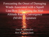
Deep Layer Shear
Deep layer shear = 0-6 km shear vector
40+ kt suggests -- if storms develop -- supercells
are likely
30-40 kt -- supercells also possible if
environment is very or extremely unstable
About 15-20 kt shear needed for organized
convection with mid level winds at least 25 kt

0-6 km Shear Vector

Craven/Brooks 0-1km Vector Shear
0-1 km AGL Vector Shear
Considerable overlap except for
sig. tornadoes
Seasonal Variation

Edwards/Thompson 0-1 km SRH

0-1 km SRH

Craven/Brooks MLLCL Heights
Mean Layer LCL Height
Again, isolates sig. Tornado from
all other classes
Seasonal Variation

Thompson/Edwards MLLCL Heights

MLLCL Heights

Craven/Brooks Findings
• MLCAPE and 0-6 km shear did not discriminate
between various classes of significant hail, wind, and
tornado events
•Best discriminators between significant tornadoes (F2-
F5) and all other classes were 0-1 km vector shear and
MLLCL heights

Thompson/Edwards Findings
• Used RUC-2 analysis proximity soundings, but results
consistent with Craven/Brooks findings
•0-6 km shear is a good discriminator between supercells and nonsupercells
•0-1 km SRH and MLLCL showed best discrimination between supercells
producing significant tornadoes and other event classes
• Application of parameter assessment depends on convective
mode (discrete cells versus lines/multicell complexes).

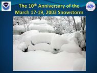
SIMILAR SOUNDINGS - DIFFERENT CONVECTIVE EVENTS
18 UTC BMX 16 Dec 2000 18 UTC BMX 16 Feb 2001

Two SPC Experimental
Research Derived Products
Supercell Composite Parameter (SCP)
Significant Tornado Parameter (STP)

Supercell Composite Parameter (SCP)
** Designed to identify areas for supercell
development
** Incorporates: MUCAPE (lowest 300 mb)
0-3 km SRH, and
BRN denominator (1/2U**2)

SCP Equation
Applied to over 500 proximity soundings (458 supercell,
75 non supercell cases)
SCP = (MUCAPE/1000 J/kg) x 0-3 km SRH/150
m**2/s**2 x (0-6 km BRN shear term/40 m**2/s**2)
If MUCAPE = 1000 J/kg; SRH = 150 M**2/S**2; BRN
shear term = 40 m**2/s**2 , then SCP = 1
> 1 for supercells;

Example of SCP Graphic

Significant Tornado Parameter (STP)
Parameters include:
1) 0-6 km AGL vector shear
2) MLCAPE (lowest 100 mb)
3) 0-1km SRH
4) MLLCL Height
5) MLCIN

STP Equation
STP = (MLCAPE/1000 J/kg) x (0-6 km vector
shear/20 m/s) x (0-1 km SRH/100 m**2/s**2) x
(2000-MLLCL/1500 m) x (150 - MLCIN/125 J/kg)
STP = 1 when, MLCAPE =1000 J/kg, 0-6km shear =20 m/s,
0-1 km shear = 100 m**2/s**2, MLLCL = 500 m, and
MLCIN=25 J/kg

STP Considerations
STP = (MLCAPE/1000 J/kg) x (0-6 km vector shear/20
m/s) x (0-1 km SRH/100 m**2/s**2) x (2000-
MLLCL/1500 m) x (150 - MLCIN/125 J/kg)
** STP approaches zero as any shear or CAPE values nears zero
** STP approaches zero as LCL height increases to 2000m
** STP approaches zero as CIN increases to 150 J/kg
MLCIN most useful prior to storm initiation

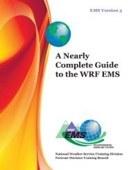
Example of STP

Mesoanalysis Summary
•Use all available resources to aid in surface analysis
(surface observations, mesonet data, satellite, radar,
profilers, etc)
•Continuity is extremely critical for mesoanalysis;
should be done hourly, if possible
•Mesoanalysis is an important part of the severe
weather evaluation process

Research Summary
•Proximity sounding research has aided SPC in better tools
to identify areas for severe storm potential
•Research has shown low MLLCL heights and strong 0-1 km
SRH/shear vector are best predictors for stronger tornadoes
(all other environmental conditions being equal)
• 30-40+ kt 0-6 km shear is favorable for supercells
•However, information misleading if initiation/ evolution of
convective mode is not accurately forecast