principles of extraction and the extraction of semivolatile organics ...

54 principles of extraction
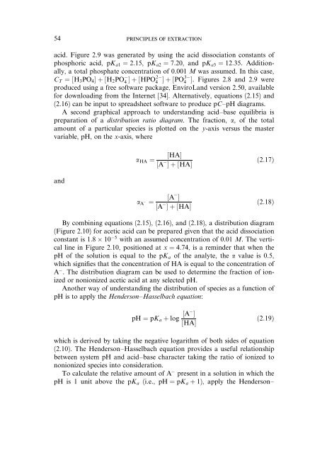
acid. Figure 2.9 was generated by using the acid dissociation constants of
phosphoric acid, pKa1 ¼ 2:15, pKa2 ¼ 7:20, and pKa3 ¼ 12:35. Additionally,
a total phosphate concentration of 0.001 M was assumed. In this case,
CT ¼½H3PO4Šþ½H2PO4 Šþ½HPO 2
4 Šþ½PO3 4 Š. Figures 2.8 and 2.9 were
produced using a free software package, EnviroLand version 2.50, available
for downloading from the Internet [34]. Alternatively, equations (2.15) and
(2.16) can be input to spreadsheet software to produce pC–pH diagrams.
A second graphical approach to understanding acid–base equilibria is
preparation of a distribution ratio diagram. The fraction, a, of the total
amount of a particular species is plotted on the y-axis versus the master
variable, pH, on the x-axis, where
and
aHA ¼
aA ¼
½HAŠ
½A Šþ½HAŠ
½A Š
½A Šþ½HAŠ
ð2:17Þ
ð2:18Þ
By combining equations (2.15), (2.16), and (2.18), a distribution diagram
(Figure 2.10) for acetic acid can be prepared given that the acid dissociation
constant is 1:8 10 5 with an assumed concentration of 0.01 M. The vertical
line in Figure 2.10, positioned at x ¼ 4:74, is a reminder that when the
pH of the solution is equal to the pKa of the analyte, the a value is 0.5,
which signifies that the concentration of HA is equal to the concentration of
A . The distribution diagram can be used to determine the fraction of ionized
or nonionized acetic acid at any selected pH.
Another way of understanding the distribution of species as a function of
pH is to apply the Henderson–Hasselbach equation:
pH ¼ pKa þ log
½A Š
½HAŠ
ð2:19Þ
which is derived by taking the negative logarithm of both sides of equation
(2.10). The Henderson–Hasselbach equation provides a useful relationship
between system pH and acid–base character taking the ratio of ionized to
nonionized species into consideration.
To calculate the relative amount of A present in a solution in which the
pH is 1 unit above the pKa (i.e., pH ¼ pKa þ 1), apply the Henderson–