Radio Interferometry Basics - NRAO
Radio Interferometry Basics - NRAO
Radio Interferometry Basics - NRAO

You also want an ePaper? Increase the reach of your titles
YUMPU automatically turns print PDFs into web optimized ePapers that Google loves.
<strong>Interferometry</strong> <strong>Basics</strong><br />
Andrea Isella<br />
Caltech<br />
Caltech CASA <strong>Radio</strong> Analysis Workshop<br />
Pasadena, January 19, 2011
1. <strong>Interferometry</strong> principles:<br />
-‐ uv plane and visibiliHes.<br />
-‐ angular resoluHon.<br />
2. Aperture Synthesis<br />
-‐ synthesized beam.<br />
-‐ characterisHc angular scales.<br />
Outline<br />
3. Data calibraHon , i.e., correcHng for the atmospheric and instrumental terms in the<br />
visibility (introducHon to Lazio’s and Perez’s talks)<br />
4. From visibiliHes to images (introducHon to Carpenter’s talk):<br />
-‐ weighHng funcHon<br />
-‐ deconvoluHon<br />
Andrea Isella :: CASA <strong>Radio</strong> Analysis Workshop :: Caltech, January 19, 2012
From Sky Brightness to Visibility<br />
1. An Interferometer measures the interference paTern produced by two<br />
apertures.<br />
2. The interference paTern is directly related to the source brightness. In parHcular,<br />
for small fields of view the complex visibility, V(u,v), is the 2D Fourier transform<br />
of the brightness on the sky, T(x,y)<br />
Fourier space/domain<br />
Image space/domain<br />
image plane<br />
(van CiTert-‐Zernike theorem) x<br />
T(x,y)<br />
uv plane<br />
Andrea Isella :: CASA <strong>Radio</strong> Analysis Workshop :: Caltech, January 19, 2012<br />
y
1<br />
b 2<br />
Visibility and Sky Brightness<br />
phase<br />
Δθ=λ/b<br />
€<br />
|V|<br />
1<br />
0.5<br />
0<br />
b 2<br />
b 1<br />
b (meters)<br />
V =<br />
The visibility is a complex quanHty:<br />
-‐ amplitude tells “how much” of a certain frequency<br />
component<br />
-‐ phase tells “where” this component is located<br />
Imax − Imin =<br />
Imax +Imin Fringe Amplitude<br />
Average Intensity<br />
Andrea Isella :: CASA <strong>Radio</strong> Analysis Workshop :: Caltech, January 19, 2012
Visibility and Sky Brightness<br />
b 1<br />
€<br />
V<br />
1<br />
0.5<br />
0<br />
b 3<br />
b 2<br />
b 1<br />
b (meters)<br />
V =<br />
The visibility is a complex quanHty:<br />
-‐ amplitude tells “how much” of a certain frequency<br />
component<br />
-‐ phase tells “where” this component is located<br />
Imax − Imin =<br />
Imax +Imin Fringe Amplitude<br />
Average Intensity<br />
Andrea Isella :: CASA <strong>Radio</strong> Analysis Workshop :: Caltech, January 19, 2012
Angular resoluHon of an interferometer<br />
b 1<br />
b<br />
Δθ=λ/2b Δθ=λ/b<br />
€<br />
A source is resolved when the visibility goes<br />
to zero on the longest baseline.<br />
For example, in the case of a binary system,<br />
this corresponds to the angular separaHon of<br />
θ = λ/2B.<br />
V = I max − I min<br />
I max +I min<br />
= 0<br />
Andrea Isella :: CASA <strong>Radio</strong> Analysis Workshop :: Caltech, January 19, 2012
Need for high angular resoluHon<br />
CARMA A-‐array configuraHon<br />
θ = 0.15’’ at 1.3 mm<br />
Single telescope Array of N telescopes<br />
Angular resoluHon, θ ~ λ/D ~λ/D max<br />
CollecHng area ~ D 2 ~ ND 2<br />
θ (‘’)<br />
10 -‐3 10 -‐2 10 -‐1 10 0 10 1 10 2<br />
CARMA<br />
SMA PdBI<br />
10<br />
λ (μm)<br />
-‐1 100 101 102 103 104 Andrea Isella :: CASA <strong>Radio</strong> Analysis Workshop :: Caltech, January 19, 2012
T(x,y)<br />
Gaussian<br />
2D Fourier Transform Pairs<br />
|V(u,v)|<br />
δ Function Constant<br />
Andrea Isella :: CASA <strong>Radio</strong> Analysis Workshop :: Caltech, January 19, 2012<br />
Gaussian
T(x,y)<br />
elliptical<br />
Gaussian<br />
2D Fourier Transform Pairs<br />
sharp edges result in many high spatial frequencies<br />
|V(u,v)|<br />
elliptical<br />
Gaussian<br />
Disk Bessel<br />
Andrea Isella :: CASA <strong>Radio</strong> Analysis Workshop :: Caltech, January 19, 2012
Aperture Synthesis<br />
V(u,v) can be measured on a discrete number of points. A good image quality<br />
requires a good coverage of the uv plane. We can use the earth rotaHon to<br />
increase the uv coverage<br />
Andrea Isella :: CASA <strong>Radio</strong> Analysis Workshop :: Caltech, January 19, 2012
CARMA ObservaHons of Mars<br />
Andrea Isella :: CASA <strong>Radio</strong> Analysis Workshop :: Caltech, January 19, 2012<br />
11
Discrete sampling:<br />
Synthesized beam<br />
T ʹ′ (x, y) = W (u,v)V (u,v)e 2πi(uv +vy) ∫∫<br />
dudv<br />
The weigh5ng func5on W(u,v) is 0 where V is not sampled<br />
T’(x,y) is FT of the product of W and V, which is the convoluHon of the FT of V<br />
and W: €<br />
T ʹ′ (x, y) = B(x, y) ⊗ T(x, y)<br />
B(x,y) is the € synthesized beam, analogous of the point-‐spread func5on in an<br />
op5cal telescope.<br />
€<br />
B(x, y) = W (u,v)e 2πi(uv +vy ) ∫∫<br />
dudv<br />
Andrea Isella :: CASA <strong>Radio</strong> Analysis Workshop :: Caltech, January 19, 2012
Effects of a sparse uv coverage<br />
Synthesized Beam (i.e.,PSF) for 2 Antennas<br />
Andrea Isella :: CASA <strong>Radio</strong> Analysis Workshop :: Caltech, January 19, 2012<br />
13
Effects of a sparse uv coverage<br />
3 Antennas<br />
Andrea Isella :: CASA <strong>Radio</strong> Analysis Workshop :: Caltech, January 19, 2012<br />
14
Effects of a sparse uv coverage<br />
4 Antennas<br />
Andrea Isella :: CASA <strong>Radio</strong> Analysis Workshop :: Caltech, January 19, 2012<br />
15
Effects of a sparse uv coverage<br />
5 Antennas<br />
Andrea Isella :: CASA <strong>Radio</strong> Analysis Workshop :: Caltech, January 19, 2012<br />
16
Effects of a sparse uv coverage<br />
6 Antennas<br />
Andrea Isella :: CASA <strong>Radio</strong> Analysis Workshop :: Caltech, January 19, 2012<br />
17
Effects of a sparse uv coverage<br />
7 Antennas<br />
Andrea Isella :: CASA <strong>Radio</strong> Analysis Workshop :: Caltech, January 19, 2012<br />
18
Effects of a sparse uv coverage<br />
8 Antennas<br />
Andrea Isella :: CASA <strong>Radio</strong> Analysis Workshop :: Caltech, January 19, 2012<br />
19
Effects of a sparse uv coverage<br />
8 Antennas x 6 Samples<br />
Andrea Isella :: CASA <strong>Radio</strong> Analysis Workshop :: Caltech, January 19, 2012<br />
20
Effects of a sparse uv coverage<br />
8 Antennas x 30 Samples<br />
Andrea Isella :: CASA <strong>Radio</strong> Analysis Workshop :: Caltech, January 19, 2012<br />
21
Effects of a sparse uv coverage<br />
8 Antennas x 60 Samples<br />
Andrea Isella :: CASA <strong>Radio</strong> Analysis Workshop :: Caltech, January 19, 2012<br />
22
Effects of a sparse uv coverage<br />
8 Antennas x 120 Samples<br />
Andrea Isella :: CASA <strong>Radio</strong> Analysis Workshop :: Caltech, January 19, 2012<br />
23
Effects of a sparse uv coverage<br />
8 Antennas x 240 Samples<br />
Andrea Isella :: CASA <strong>Radio</strong> Analysis Workshop :: Caltech, January 19, 2012<br />
24
Effects of a sparse uv coverage<br />
8 Antennas x 480 Samples<br />
The synthesized beam approaches a 2D gaussian funcHon<br />
and can be described in terms of its Full Width at Half<br />
Maximum (FWHM) and PosiHon Angle (PA)<br />
Andrea Isella :: CASA <strong>Radio</strong> Analysis Workshop :: Caltech, January 19, 2012<br />
25
CharacterisHc angular scales<br />
1. An interferometer has at least THREE important characterisHc angular scales:<br />
-‐ angular resoluHon: ~ λ/D max , where D max is the maximum separaHon<br />
between the apertures.<br />
-‐ shortest spacing problem: the source is resolved if θ>λ/D min , where D min is<br />
the minimum separaHon between apertures.<br />
An interferometer is sensi5ve to a range of angular sizes, λ/D max -‐ λ/D min<br />
and<br />
since D min > Aperture diameter, an interferometer is not sensiHve to the large<br />
angular scales and cannot recover the total flux of resolved sources (you need<br />
a single dish, e.g., CSO, APEX, IRAM 30 m, ALMA total power array, CCAT) .<br />
2. Field of view of the single aperture ~ λ/D, where D is the diameter of the<br />
telescope. Source more extended than the field of view can be observed<br />
using mulHple poinHng centers in a mosaic.<br />
Andrea Isella :: CASA <strong>Radio</strong> Analysis Workshop :: Caltech, January 19, 2012
Primary beam and Field of View<br />
A telescope does not have uniform response across the enHre sky<br />
-‐ main lobe approximately Gaussian, fwhm ~1.2λ/D = “primary beam”<br />
-‐ limited field of view ~ λ/D<br />
Andrea Isella :: CASA <strong>Radio</strong> Analysis Workshop :: Caltech, January 19, 2012
CharacterisHc angular scales for the EVLA<br />
Andrea Isella :: CASA <strong>Radio</strong> Analysis Workshop :: Caltech, January 19, 2012
CharacterisHc angular scales during<br />
ALMA early science<br />
Dmax = 400 m, Dmin = 30 m, D = 12 m<br />
Band λ λ/D max λ/D min FOV<br />
3 3 mm 1.5’’ 10.5’’ 50’’<br />
6 1.3 mm 0.6’’ 4.5’’ 22’’<br />
7 0.9 mm 0.4’’ 3.0’’ 15’’<br />
9 0.45 mm 0.2’’ 1.5’’ 8’’<br />
1. How complex is the source? Is good (u,v) coverage needed? This may set<br />
additional constraints on the integration time if the source has a complex<br />
morphology. <br />
2. How large is the source? If it is comparable to the primary beam (λ/D), you<br />
should mosaic several fields#<br />
Andrea Isella :: CASA <strong>Radio</strong> Analysis Workshop :: Caltech, January 19, 2012
Measuring the visibility<br />
T ν ʹ′ (x, y) = Wν (u,v)V ν (u,v)e 2πi(uv +vy) ∫∫<br />
dudv<br />
CalibraHon formula:<br />
€ V ˜<br />
ν (u,v) = Gν (u,v)V ν (u,v) +εν (u,v) +ην (u,v)<br />
€<br />
G(u,v) = complex gain, i.e., amplitude and phase gains.<br />
Due to the atmosphere, i.e., different opHcal path and atmospheric<br />
opacity, and to the instrumental response to the astronomical<br />
signal.<br />
ε(u,v) = complex offset, i.e., amplitude and phase offset. Engineers<br />
work hard to make this term close to zero<br />
η(u,v) = random complex noise<br />
Andrea Isella :: CASA <strong>Radio</strong> Analysis Workshop :: Caltech, January 19, 2012
Data CalibraHon<br />
Basic idea: observe sources with known flux, shape and spectrum to derive the response of<br />
the instrument.<br />
Bandpass calibra5on:<br />
what does it do? It compensates for the change of gain with frequency.<br />
How does it work? A strong source with a flat spectrum (i.e., bandpass calibrator) is<br />
observed (usually once during the track). Bandpass calibraHon is generally stable across the<br />
track.<br />
Phase calibra5on:<br />
What does it do? It compensates for relaHve temporal variaHon of the phase of the<br />
correlated signal on different antennas (or baselines).<br />
How does it work?<br />
-‐ using Water Vapor <strong>Radio</strong>meters (see Laura’s talk)<br />
-‐ a strong source with known shape (preferably a point source) is observed every few<br />
minutes. If the gain calibrator is a point source, than the gain are derived assuming that the<br />
intrinsic phase is 0.<br />
Andrea Isella :: CASA <strong>Radio</strong> Analysis Workshop :: Caltech, January 19, 2012
Data CalibraHon<br />
Basic idea: observe sources with known flux, shape and spectrum to derive the response of<br />
the instrument.<br />
Amplitude calibra5on:<br />
What does it do? It compensates for atmospheric opacity and loss of signal within the<br />
interferometer (e.g., poinHng errors).<br />
How does it work? A source with known flux is observed. This can be a planet for which<br />
accurate models exists, or a *stable* radio source, which has been independently calibrated<br />
using, e.g., a planet. Accuracies < 15% in the absolute flux are challenging and might<br />
required specific observing strategies.<br />
Andrea Isella :: CASA <strong>Radio</strong> Analysis Workshop :: Caltech, January 19, 2012<br />
Hme
<strong>Radio</strong>-‐Frequency Interference (RFI)<br />
RFI mainly affect low frequency observaHons<br />
RFI in L-‐band from 1 to 2 GHz<br />
hTp://evlaguides.nrao.edu/index.php?Htle=ObservaHonal_Status_Summary<br />
Andrea Isella :: CASA <strong>Radio</strong> Analysis Workshop :: Caltech, January 19, 2012
<strong>Radio</strong>-‐Frequency Interference (RFI)<br />
RFI in S-‐band from 2 to 3 GHz<br />
hTp://evlaguides.nrao.edu/index.php?Htle=ObservaHonal_Status_Summary<br />
Andrea Isella :: CASA <strong>Radio</strong> Analysis Workshop :: Caltech, January 19, 2012
<strong>Radio</strong>-‐Frequency Interference (RFI)<br />
1. Avoid the frequencies affected by RFI.<br />
Check hTp://evlaguides.nrao.edu/index.php?Htle=ObservaHonal_Status_Summary<br />
For a complete list of known RFI<br />
2. If you cannot avoid RFI, try to observe in the extended configuraHons, where<br />
RFI are less severe<br />
3. Apply spectral smoothing to the data, but in general you will not be able to get<br />
Useful data within a few MHz from the RFI frequency,<br />
Andrea Isella :: CASA <strong>Radio</strong> Analysis Workshop :: Caltech, January 19, 2012
From visibiliHes to images (see also John’s talk<br />
tomorrow)<br />
• uv plane analysis<br />
– best for “simple” sources, e.g. point sources, disks<br />
• image plane analysis<br />
– Fourier transform V(u,v) samples to image plane, get T ’ (x,y)<br />
– but difficult to do science on dirty image<br />
– deconvolve b(x,y) from T ’ (x,y) to determine (model of) T(x,y)<br />
visibilities dirty image sky brightness<br />
Andrea Isella :: CASA <strong>Radio</strong> Analysis Workshop :: Caltech, January 19, 2012
Measured flux:<br />
Synthesized beam:<br />
WeighHng funcHon<br />
€<br />
T ʹ′ (x, y) = B(x, y) ⊗ T(x, y)<br />
B(x, y) = W (u,v)e 2πi(uv +vy ) ∫∫<br />
dudv<br />
You can change the angular resolu5on and<br />
sensi5vity € of the final image by changing the<br />
weigh5ng func5on W(u,v)<br />
Andrea Isella :: CASA <strong>Radio</strong> Analysis Workshop :: Caltech, January 19, 2012
WeighHng funcHon<br />
• “Natural” weighHng: W(u,v) = 1/σ 2 (u,v), where σ 2 (u,v) is the noise variance<br />
of the (u,v) sample:<br />
Advantage: gives the lowest noise in the final image, highlight extended<br />
structures.<br />
Disadvantage: generally gives more weights to the short baseline (where<br />
there are more measurements of V) degrading the resoluHon<br />
• “Uniform” weighHng: W(u,v) is inversely proporHonal to the local density of<br />
(u,v) points. It generally gives more weights to the long baseline therefore<br />
leading to higher angular resoluHon.<br />
Advantage: beTer resoluHon and lower sidelobes<br />
Disadvantage: higher noise in the final map<br />
• “Robust” (Briggs) weighHng: W(u,v) depends on a given threshold value S,<br />
so that a large S gives natural weighHng and a small S gives uniform weighHng.<br />
Advantage: conHnuous variaHon of the angular resoluHon.<br />
Andrea Isella :: CASA <strong>Radio</strong> Analysis Workshop :: Caltech, January 19, 2012
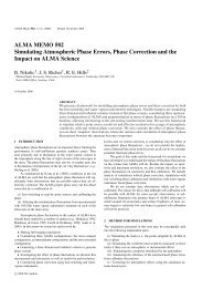
NATURAL WEIGHTING<br />
WeighHng funcHon<br />
FWHM beam size = 1.7’’ x 1.2’’ 0.21’’ x 0.19’’<br />
Andrea Isella :: CASA <strong>Radio</strong> Analysis Workshop :: Caltech, January 19, 2012<br />
UNIFROM WEIGHTING
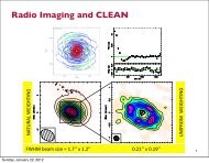
DeconvoluHon: Dirty Vs Clean image<br />
A non complete coverage of the uv plane<br />
gives a synthesized beam with a lot of<br />
sidelobes, i.e. a ‘dirty’ beam. And since<br />
T ʹ′ (x, y) = B(x, y) ⊗ T(x, y)<br />
T’(x,y) is also characterized by sidelobes,<br />
i.e., ‘dirty’ image.<br />
,<br />
The deconvolu5on process consists in giving reasonable values to the visibility in the<br />
unmeasured (u,v) areas in order to get a nice gaussian beam without sidelobes. The<br />
most successful deconvoluHon procedure is the algorithm CLEAN (Hogbom 1974).<br />
Deconvolu5on or Cleaning<br />
Dirty image Clean image<br />
Andrea Isella :: CASA <strong>Radio</strong> Analysis Workshop :: Caltech, January 19, 2012
Concluding remarks. I<br />
• <strong>Interferometry</strong> samples visibiliHes that are related to a sky brightness image<br />
by the Fourier transform.<br />
Keep in mind these three important scales:<br />
-‐ angular resoluHon ~ λ/maximum baseline ,<br />
-‐ largest mapped spaHal scale ~ λ/minimum baseline<br />
-‐ field of view ~ λ/antenna diameter<br />
Also note that to have “good” images you need a “good” sampling of the uv<br />
plane<br />
• The measured visibiliHes contains wavelength-‐dependent atmospheric and<br />
instrumental terms. The “data reducHon” consists in deriving these terms<br />
from the observaHons of sources with known spectrum, shape and flux.<br />
Re-‐reducing the same dataset 10 Hmes is fine!<br />
Andrea Isella :: CASA <strong>Radio</strong> Analysis Workshop :: Caltech, January 19, 2012
Concluding remarks. II<br />
• Once you have calibrated your data, keep in mind that there is an infinite<br />
number of images compaHble with the sampled visibiliHes. Play around with<br />
the weighHng funcHons while using CASA<br />
• DeconvoluHon (e.g. cleaning) try to correct for the incomplete sampling of<br />
the uv-‐plane. Play around with ‘clean’ while using CASA<br />
Andrea Isella :: CASA <strong>Radio</strong> Analysis Workshop :: Caltech, January 19, 2012
References<br />
• Thompson, A.R., Moran, J.M., & Swensen, G.W. 2004, “<strong>Interferometry</strong> and<br />
Synthesis in <strong>Radio</strong> Astronomy” 2nd ediHon (WILEY-‐VCH)<br />
• <strong>NRAO</strong> Summer School proceedings<br />
– hTp://www.aoc.nrao.edu/events/synthesis/2010/lectures10.html<br />
– Perley, R.A., Schwab, F.R. & Bridle, A.H., eds. 1989, ASP Conf. Series 6, Synthesis<br />
Imaging in <strong>Radio</strong> Astronomy (San Francisco: ASP)<br />
• Chapter 6: Imaging (Sramek & Schwab), Chapter 8: DeconvoluHon (Cornwell)<br />
• IRAM Summer School proceedings<br />
– hTp://www.iram.fr/IRAMFR/IS/archive.html<br />
– Guilloteau, S., ed. 2000, “IRAM Millimeter <strong>Interferometry</strong> Summer School”<br />
• Chapter 13: Imaging Principles, Chapter 16: Imaging in PracHce (Guilloteau)<br />
– J. Pety 2004, 2006, 2008 Imaging and DeconvoluHon lectures<br />
• CARMA Summer School proceedings<br />
- hTp://carma.astro.umd.edu/wiki/index.php/School2010<br />
- CARMA SUMMER school, July 2011, ask J. Carpenter for informaHon<br />
Andrea Isella :: CASA <strong>Radio</strong> Analysis Workshop :: Caltech, January 19, 2012