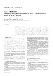
Radio Imaging and CLEAN - NRAO

Radio Imaging and CLEAN 

!"#$%"&'()*+,#*!+' 

Sunday, January 22, 2012 

-(,/'0123'4561'7'89:;;'9=8;;'

Credits 

• Slides borrowed from : 

– https://science.nrao.edu/facilities/alma/naasc-workshops/almadata/indebetouw.pdf 

• “Imaging ALMA Data” by Remy Indebetouw 

• In turn borrowed from David Wilner, Steve Myers, and Scott Schnee 

– http://www.almatelescope.ca/workshop/Talks/CASAImaging_Hamilton.pdf 

• “Imaging with CASA” by Crystal Brogan 

– http://www.aoc.nrao.edu/events/synthesis/2010/lectures/wilner_synthesis10.pdf 

• “Imaging and Deconvolution” by David Wilner @ VLA Summer School 

– http://www.das.inpe.br/school/2011/lectures/RickPerley_Lecture4.pdf 

• “Imaging and Deconvolution” by Rick Perley 

• General references 

– Thompson, A.R., Moran, J.M., & Swensen, G.W., “Interferometry and Synthesis in 

Radio Astronomy” 

– VLA Summer School Lectures (available online) 


2

Outline 

• Brief review of synthesis imaging 

• Demonstration of deconvolution (i.e, “clean”) 

• CASA clean - basics 

– images 

– imsize, cell size, mode, mask 

– when to stop cleaning 

– weighting 

• CASA clean - advanced topics 

– multiscale clean 

– combining interferometry data with single dish 

– self-calibration 

– mosaicking 


3

From Sky Brightness to Visibility 

1. An interferometer measures the interference pattern produced by 

two apertures. 

2. The interference pattern is directly related to the source brightness. 

For small fields of view the complex visibility, V(u,v), is the 2D 

Fourier transform of the brightness on the sky, T(l,m) 

van Cittert-Zernike theorem 

Fourier space/domain 

Image space/domain 


image plane 

l 

uv plane 

T(l,m) 

4 

m

Imaging and Deconvolution 

• Consequences of finite uv coverage 

– no data beyond umax, vmax → unresolved structure 

– no data within umin, vmin → limit on largest size scale 

– holes between umin,vmin and umax, vmax → sidelobes 

• Empty (u,v) cells can have ANY value 

• Noise → undetected/corrupted structure in T(l,m) 

• Interpolate/extrapolate observed V(u,v) values to fill in empty 

uv cells 

An infinite number of T(l,m) compatible with observed V(u,v) 


8

Deconvolution Algorithms 

• CLEAN (Högbom 1974) 

– assumes T(l,m) is a collection of point sources 

– multi-scale CLEAN relaxes this assumption 

• Maximum Entropy (Gull & Skilling 1983) 

– assumes T(l,m) is smooth and positive 

• Beam shape 

– needed to deconvolve image 

– atmospheric seeing can modify effective beam shape 


9

• Find brightest points in dirty image 


10


• Create model image containing a 

fraction of those flux points 


11




• Subtract model from data, 

leaving a residual 


12




• Subtract model from data, 

leaving a residual 

• Final product = residual + model 

(convolved with restoring 

Gaussian beam) 


13


residual (log scale) model convolved w/ restorimg beam (log scale) 

residual (linear scale) 

cleaned image (log scale) 

14


residual (log scale) model convolved w/ restoring beam (log scale) 


restrict where the algorithm 

can search for clean 

components, with a mask 


15


residual (log scale) model convolved w/ restoring beam 


10 iterations 


16




20 iterations 


17




30 iterations 


18




40 iterations 


19




50 iterations 


20




60 iterations 


21




70 iterations 


22




80 iterations 


23




90 iterations 


24




100 iterations 


25






26






27






28






29






30






31






32






33

Deconvolution 

Results depend on: 

• image parameters: size, cell, weighting, gridding, mosaic 

• deconvolution parameters: algorithm, iterations, boxing, stopping criteria 


dirty image (log scale) 


34

CASA: inputs to “clean” 


35

imagename 


36

imagename 

• .image 

– final cleaned image (or dirty image if niter=0) 

• .psf 

– point spread function, or “dirty beam” 

• .model 

– image of the clean components 

• .residual 

– residual image after subtracting clean components 

– check to see if more cleaning is needed 

• .flux 

– relative sky sensitivity over field 

– pbcor=True divides the .image by the .flux 

– higher noise at edge of image 


37

imsize and cell 


38

imsize and cell 

• cell 

– should satisfy sampling theorem for the longest baselines, 

Δx < 1/(2 u max ), Δy < 1/(2 v max ) 

– in practice, 3 to 5 pixels across the main lobe of the dirty beam 

• imsize 

– natural resolution in (u,v) plane samples FT{A(x,y)}, implies image size 

2x primary beam 

– primary bean ~ 1.2 * λ/D, D = telescope diameter 

– e.g., ALMA: 870 µm, 12 m telescope → 2 x 18 arcsec 

* not restricted to powers of 2 (in fact internal padding complicates) 

* if there are bright sources in the sidelobes of A(x,y), then they will be 

aliased into the image (need to make a larger image) 


39

plotuv 


40

im.advise 


0.5/maxuv – absolute minimum; 

recommend < 0.2/maxuv = 1.1arcsec 

41

mode 


42

mode 

• mode = mfs (multi-frequency synthesis) 

– sum each channel to make a continuum image 

– nterm: models the sky-frequency dependence of the continuum 

• mode = channel, velocity, or frequency 

– data: taken in sky frequency (terrestrial, TOPO) frame 

• velocity: include doppler shifts from: 

– Earth rotation: few km/s (diurnal) 

– Earth orbit: 30 km/s (annual) 

– Earth/Sun motion w.r.t. LSR (e.g. LSRK, LSRD) 

– maybe galactic rotation to extragalactic frames 

– imaging applies doppler corrections on the fly, works in LSRK 

– you choose the subsequent output cube parameters 

• nchan, start, width specify which channels to image 

– can shift and regrid data before imaging using cvel 


43

When to stop cleaning? : niter & threshold 


44

When to stop cleaning? : niter & threshold 

• niter 

– Maximum number of clean interations to perform. 

– Set niter=0 for dirty map OR set to large number 

– use “threshold” to terminate cleaning 

• threshold 

– stop cleaning when peak residual has this value 

– set to multiple of rms noise if noise-limited 

OR 

fraction of brightest source peak flux if dynamic range limited 


45

mode 


46

Dirty Beam Shape –1– and Weighting 

• introduce weighting function W(u,v) 

S(l, m) =F −1 {W (u, v) × S(u, v)} 

– W modifies dirty beam 

• “Natural” weighting 

– W(u,v) = 1/σ 2 (u,v) at points with data and 

zero elsewhere, where σ 2 (u,v) is the noise 

variance of the (u,v) sample 

– maximizes point source sensitivity 

– (lowest rms in image) 

– generally more weight to short baselines (large 

spatial scales), degrades resolution 


47

Dirty Beam Shape and Weighting 

• “Uniform” weighting 

– W(u,v) is inversely proportional to local 

density of (u,v) points 

– fills (u,v) plane more uniformly, so 

(outer) sidelobes are lower 

– gives more weight to long baselines and 

therefore higher angular resolution 

– degrades point source sensitivity 

(higher rms in image) 

– can be trouble with sparse sampling: 

cells with few data points have same weight 

as cells with many data points 


48


• “Robust” (Briggs) weighting 

– variant of “uniform” that avoids giving too much 

weight to cell with low natural weight 

– an adjustable parameter that allows for 

continuous variation between highest angular 

resolution and optimal point source sensitivity 

– large threshold → natural weighting 

– small threshold → uniform weighting 

– robust ~ 0 to 1 gives good results 


49


• “Tapering” 

– apodize the (u,v) sampling by a Gaussian 

t = tapering parameter (in kλ; arcsec) 

– like smoothing in the image plane (convolution 

by a Gaussian) 

– gives more weight to short baselines, degrades 

angular resolution 

– degrades point source sensitivity but can 

improve sensitivity to extended structure 


50

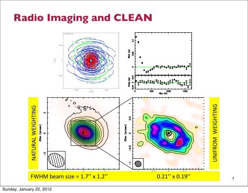
Example of Natural vs. Uniform Weighting 

!"#$%"&'()*+,#*!+' 


-(,/'0123'4561'7'89:;;'9=8;;'

Weighting and Tapering: Summary 

• imaging parameters provide a lot of freedom 

• appropriate choice depends on science goals 

Robust/Uniform Natural Taper 

Resolution higher medium lower 

Sidelobes lower higher depends 

Point Source 

Sensitivity 

Extended Source 

Sensitivity 


lower maximum lower 

lower medium higher 

52

mask 


53

mask 

• Define region where you expect the emission to be 

• CLEAN components will fall within the masked region 

• can also define with interactive=True 


54

Interactive Clean 

residual image in viewer 

define a mask with R-click on 

shape type 

define the same mask for all 

channels 

or iterate through the channels 

with the tape deck and define 

separate masks 


55

nteractive Clean 

perform N iterations 

and return – every time the 

residual is displayed is a major 

cycle 

continue until #cycles 

or threshold reached, 

or user stop 


56

multiscale clean 

• Models the sky using components with different size scales 

• multiscale = [0,5,15,45] 

– scales are in units of pixels 

– 0=point, typically 1-2x synthesized beam, then multiples of 2-3x that up to 

a fraction of the PB can be tricky to get to work right 

• Yields promising results on extended sources 

• See, e.g., Rich et al. 2008, AJ, 136, 2897 for comparison between clean and 



57



multiscale “classic” 1-scale 

58

zero-spacing 

Low Spatial Frequencies (I) 

• Large Single Telescope 

– make an image by scanning across the sky 

– all Fourier components from 0 to D sampled, where D is the 

telescope diameter (weighting depends on illumination) 

– Fourier transform single dish map = T(x,y) $ A(x,y), then divide 

by a(x,y) = FT{A(x,y)}, to estimate V(u,v) 

– choose D large enough to overlap interferometer samples of 

V(u,v) and avoid using data where a(x,y) becomes small 


density of 

uv points 

(u,v) 

63 

59

zero-spacing 

Low Spatial Frequencies (II) 

• separate array of smaller telescopes 

– use smaller telescopes observe short baselines not 

accessible to larger telescopes 

– shortest baselines from larger telescopes total power maps 


ALMA with ACA 

50 x 12 m: 12 m to 14 km 

+12 x 7 m: fills 7 to 12 m 

+ 4 x 12 m: fills 0 to 7 m 

64 

60

self calibration 

• phase calibration is not perfect 

– gain solution interpolated from different time, and different location on the 

sky 

• self-calibration corrects for gain errors from on-source observations 

– N complex gains, where N = number of antennas 

– N(N-1)/2 visibilities 

– over constrained problem is N is large and source structure is simple 

– required sufficient signal-to-noise at each time interval 

• procedure 

– assume initial model 

– solve for time-dependent gains 

– form new sky model from corrected data using CLEAN 

– solve for new gains 


61

mosaicking 

• image multiple pointings of the antennas 

• imagermode = ‘mosaic’ 

• mosweight = True 

– weights pointings by sensitivity in overlap regions 

• field = ‘’ 

– selects fields to mosaic 

• ftmachine 

– ftmachine=‘mosaic’ 

• add in uv plane and invert together 

– ftmachine=’ft’ 

• shift and add in image plane 


62

Radio Imaging and CLEAN - NRAO

Create successful ePaper yourself

Delete template?

Save as template?