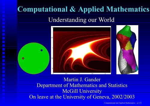
Computational & Applied Mathematics

Computational & Applied Mathematics
Understanding our World
0
0.5
1
1.5
2
0 0.5 1 1.5 2
Martin J. Gander
Department of Mathematics and Statistics
McGill University
On leave at the University of Geneva, 2002/2003
Computational and Applied Mathematics – p.1/31

Optimal Intercept Time
y
x0
Suspect Vessel: speed v
Police Boat: speed u
y0
What direction does the police boat have to choose
to approach the suspect vessel up to a distance R as
quickly as possible ?
x
Computational and Applied Mathematics – p.2/31

Geometric Solution
y
x0
y0
Imagine the police boat going into all directions at the
same time =⇒ y 2 0 + (vt − x0) 2 = (ut + R) 2 .
In “Note on the Optimal Intercept Time of Vessels to a Nonzero Range”
G, SIAM Review Vol. 40, No. 3, 1998.
R
x
Computational and Applied Mathematics – p.3/31

The Donut Problem
Top View
Side View
What is the maximum number of pieces one can get
from a donut when cutting it with three planar cuts ?
Starting with an apple, how many pieces can we get ?
Computational and Applied Mathematics – p.4/31

First Cut
Top view First cut
The most we can get with a single planar cut is two
pieces.
Computational and Applied Mathematics – p.5/31

Second Cut
Top view
First and second cut
We get six pieces in total, each of the first two is cut
twice.
Computational and Applied Mathematics – p.6/31

Third Cut
How many pieces do we have now ?
Computational and Applied Mathematics – p.7/31

The Total Number of Pieces is
4
Upper top octant:
5
3 pieces
1
2
3
Lower top octant:
2 pieces
Upper left octant:
8
6
7
Lower left octant:
1 piece
15 Pieces with 3 planar cuts.
2 pieces 1 piece
Upper right octant:
10
9
14
Lower right octant:
1 piece
Upper bottom octant:
15
11
3 pieces
12
13
Lower bottom octant:
2 pieces
Computational and Applied Mathematics – p.8/31

Is this Solution Really Correct ?
The answer is NO, the maximum number of pieces
one can get is 13 ! How ?
An article by Martin Gardner in the “Scientific
American” contains the general result for a torus in n
dimensions and m cuts along hyperplanes.
Suppose you are allowed to move the pieces between
the cuts, what is now the maximum number of pieces
you can get ?
Computational and Applied Mathematics – p.9/31

Circular Billiard
In which direction do you have to push the red ball so
that it bounces of the rim exactly once and then hits
the blue ball ?
Is there more than one solution ? Computational and Applied Mathematics – p.10/31

Circular Billiard: Algebraic Solution
PSfrag replacements
b
y
θ
−c a
f(θ) = (1 + c cos θ) (a − cos θ) 2 + (b − sin θ) 2
− (1 − a cos θ − b sin θ) (c + cos θ) 2 + (sin θ) 2
γ
1
x
Computational and Applied Mathematics – p.11/31

cements
f(θ)
Solution for the Given Example
0.4
0.3
0.2
0.1
0
−0.1
−0.2
PSfrag replacements
θ
−0.3
0 1 2 3 4 5 6 7
θ
f(θ)
Are there always four solutions ?
150
210
120
240
90
180 0
270
0.4
0.2
1
0.8
0.6
60
300
Computational and Applied Mathematics – p.12/31
30
330

The Geometric Point of View
PSfrag replacements
m2
y
−e m1
θ
α
We need to find an ellipse which touches the circle tan-
gentially.
e
1
x
Computational and Applied Mathematics – p.13/31

Number of Solutions
An example with 4 solutions and one with 2 only.
Q(u) = (m2−m2m1)u 4 +(2m1−2m 2 1 +2e2 +2m 2 2 )u3 +6u 2 m2m1
+ (−2m 2 2 + 2m 2 1 + 2m1 − 2e 2 )u − m2m1 − m2 = 0
where θ = 2 arctan(u). Q(u) is a 4th degree
polynomial, there can not be more than four solutions.
Computational and Applied Mathematics – p.14/31

Dependence on the Ball Position
A numerical experiment: fixing the position of one
ball and varying the position of the second ball.
Counting the number of solutions gives the gray
shade:
Computational and Applied Mathematics – p.15/31

Dependence on the Ball Position
The separatrix (x,y) can be computed analytically (t parameter):
x(t) = − c
h
(1 + c)t 6 + 3(1 + 3c)t 4 + 3(1 − 3c)t 2 + (1 − c) ,
y(t) = 16
h c2 t 3 , h = (1 + 3c + 2c 2 )t 6 + 3(1 + c + 2c 2 )t 4 +
+3(1 − c + 2c 2 )t 2 + (1 − 3c + 2c 2 )
where c is the position of the fixed ball on the x axis.
Computational and Applied Mathematics – p.16/31

Dependence on the Ball Position
Top view of a coffee mug with a point source of light
emulating the circular billiard game
(Drexler and G, SIAM review Vol. 40, No. 2, 1998)
Computational and Applied Mathematics – p.17/31

Digital Signal Processing
A periodic signal f(t) can be decomposed into its
Fourier components:
f(t) =
∞
k=−∞
ˆfke ikt .
Discrete version: for the vector f of length n, where
fj := f(tj), tj = j∆t, ∆t = 2π/n, we have
fj =
n−1
k=0
ˆfke iktj .
What if the signal is an image, or a piece of music?
Computational and Applied Mathematics – p.18/31

Population Dynamics
Joint work with Antonio Steiner, Il Volterriano
1997-2003
Computational and Applied Mathematics – p.19/31

The Lotka Volterra System
We consider rabbits and foxes living in a common
habitat. If x denotes the rabbit population and y the
fox population, the Lotka Volterra model states
˙x = x − xy
˙y = −y + xy
Approximating the derivative using its definition:
x(tn+1) − x(tn)
∆t
y(tn+1) − y(tn)
∆t
= x(tn) − x(tn)y(tn)
= −y(tn) + x(tn)y(tn)
We get a discrete dynamical system. Computational and Applied Mathematics – p.20/31

Solutions
The exact solutions are cycles, but in general exact
solutions can not be found. Numerical solutions
spiral:
y
2.5
2
1.5
1
0.5
0
0 0.5 1 1.5 2 2.5
x
y
3
2.5
2
1.5
1
0.5
0
0 0.5 1 1.5
x
2 2.5 3
Computational and Applied Mathematics – p.21/31

A Symplectic Method
A very small change in the original method, instead of
x(tn+1) − x(tn)
∆t
y(tn+1) − y(tn)
∆t
= x(tn) − x(tn)y(tn)
= −y(tn) + x(tn)y(tn)
changing in the second line tn to tn+1,
x(tn+1) − x(tn)
∆t
y(tn+1) − y(tn)
∆t
= x(tn) − x(tn)y(tn)
= −y(tn) + x(tn+1)y(tn)
leads to a method for which one can prove that the
approximate solution is cyclic like the exact solution.
Computational and Applied Mathematics – p.22/31

Success...
4
3.5
3
2.5
2
1.5
1
0.5
0
−1 0 1 2 3 4 5 6
The approximate solutions are also cycles, like the
mathematically exact or “biological” ones.
Computational and Applied Mathematics – p.23/31

and Failure of the new method
4
3
2
1
0
−1
−2
−25 −20 −15 −10 −5 0 5 10
4
3.5
3
2.5
2
1.5
1
0.5
0
−1 0 1 2 3 4 5 6
But here, in spite of the proof of cyclic behavior, the
method failed. On the right one can see why with the
zoom!
Computational and Applied Mathematics – p.24/31

So When does the Method Work?
0
0.5
1
1.5
2
0 0.5 1 1.5 2
The boundary beteween where the method works and
where it does not is very complicated: it is a fractal.
Computational and Applied Mathematics – p.25/31

Room Temperature in Montreal
∂u
∂t (x, t) = ∂2u ∂x2 (x, t)+ ∂2u ∂y2 (x, t)+ ∂2u ∂z
2 (x, t)+f(x, t)
Room temperature
in our living room
in Montreal (outside
temperature up to -47
degrees): the heat equation.
Insulated walls, not
well insulated windows
and doors.
Computational and Applied Mathematics – p.26/31

Why a Turntable in the Microwave ?
0.3
0.25
0.2
0.15
0.1
0.05
0
The physical model is Maxwell’s equation
∇ × E = −µHt,
∇ × H = εEt + σE
0.05 0.1 0.15 0.2 0.25 0.3 0.35 0.4 0.45 0.5
Computational and Applied Mathematics – p.27/31

Why a Turntable in the Microwave ?
0.3
0.25
0.2
0.15
0.1
0.05
0
The physical model is Maxwell’s equation
∇ × E = −µHt,
∇ × H = εEt + σE
0.05 0.1 0.15 0.2 0.25 0.3 0.35 0.4 0.45 0.5
0.3
0.25
0.2
0.15
0.1
0.05
0
0.05 0.1 0.15 0.2 0.25 0.3 0.35 0.4 0.45 0.5
Computational and Applied Mathematics – p.27/31

Noise Levels in a VOLVO S90
Noise simulation on a parallel
computer to improve
passenger comfort
14
2
6
12
10
4 3 5
8
16
7
11
15
Computational and Applied Mathematics – p.28/31
9
13
1

Radiation Therapy for Cancer
For cancer treatment it is important to have a very pre-
cise model of the body part that will be exposed to ra-
diation.
Computational and Applied Mathematics – p.29/31

Aircraft Industry: B-747 in Flight
Simulation of a B-
747 flying through a
thunderstorm, computation
of the ice
accumulation on the
wings and around
the engine intake.
Computational and Applied Mathematics – p.30/31

The Fundamental Role of CAM
Physics:
− Fluid Dynamics
− Aero Dynamics
− Radiation
− Particle Physics
Engineering:
− Circuits Simulation
− Active Noise Cancellation
− Cellular Phone Systems
0.4
0.3
0.2
0.1
0
0 0.2 0.4 0.6 0.8 1
Computational
AND
Applied Mathematics
0.9
0.8
0.7
0.6
0.5
0.4
0.3
0.2
0.1
Biology:
− Population Dynamics
− Antibiotics
− Micromachines
0
0.5
1
1.5
2
0 0.5 1 1.5 2
Pure Mathematics:
− Geometry
− Asymptotics
− Existence
See also: www.math.mcgill.ca/mgander
Computational and Applied Mathematics – p.31/31