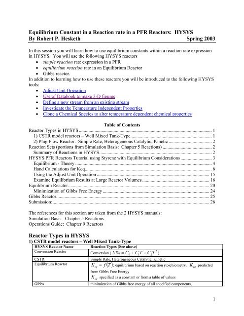
Conversion Reactors: HYSYS - Rowan

Equilibrium Constant in a Reaction rate in a PFR Reactors: HYSYS
By Robert P. Hesketh Spring 2003
In this session you will learn how to use equilibrium constants within a reaction rate expression
in HYSYS. You will use the following HYSYS reactors
• simple reaction rate expression in a PFR
• equilibrium reaction rate in an Equilibrium Reactor
• Gibbs reactor.
In addition to learning how to use these reactors you will be introduced to the following HYSYS
tools:
• Adjust Unit Operation
• Use of Databook to make 3-D figures
• Define a new stream from an existing stream
• Investigate the Temperature Independent Properties
• Clone a Chemical Species to alter temperature dependent chemical properties
Table of Contents
Reactor Types in HYSYS ............................................................................................................... 1
1) CSTR model reactors – Well Mixed Tank-Type.................................................................... 1
2) Plug Flow Reactor: Simple Rate, Heterogeneous Catalytic, Kinetic .................................... 2
Reaction Sets (portions from Simulation Basis: Chapter 5 Reactions) ......................................... 2
Summary of Reactions in HYSYS.............................................................................................. 2
HYSYS PFR Reactors Tutorial using Styrene with Equilibrium Considerations .......................... 3
Equilibrium - Theory .................................................................................................................. 4
Hand Calculations for Keq.......................................................................................................... 6
Using the Adjust Unit Operation .............................................................................................. 15
Examine Equilibrium Results at Large Reactor Volumes ........................................................ 16
Equilibrium Reactor...................................................................................................................... 20
Minimization of Gibbs Free Energy ......................................................................................... 24
Gibbs Reactor................................................................................................................................ 25
Submission:................................................................................................................................... 26
The references for this section are taken from the 2 HYSYS manuals:
Simulation Basis: Chapter 5 Reactions
Operations Guide: Chapter 9 Reactors
Reactor Types in HYSYS
1) CSTR model reactors – Well Mixed Tank-Type
HYSYS Reactor Name Reaction Types (See above)
X % = C + C T + C T
Conversion Reactor 2
Conversion ( )
CSTR Simple Rate, Heterogeneous Catalytic, Kinetic
Keq = f T ; equilibrium based on reaction stoichiometry. K predicted
Equilibrium Reactor ( )
0
from Gibbs Free Energy
K specified as a constant or from a table of values
eq
Gibbs minimization of Gibbs free energy of all specified components,
1
2
eq
1

option 1) no the reaction stoichiometry is required
option 2) reaction stoichiometry is given
2) Plug Flow Reactor: Simple Rate, Heterogeneous Catalytic, Kinetic
Taken from: 9.3 Plug Flow Reactor (PFR)
The PFR (Plug Flow Reactor, or Tubular Reactor) generally consists of a bank of cylindrical
pipes or tubes. The flow field is modeled as plug flow, implying that the stream is radially
isotropic (without mass or energy gradients). This also implies that axial mixing is negligible.
As the reactants flow the length of the reactor, they are continually consumed, hence, there will
be an axial variation in concentration. Since reaction rate is a function of concentration, the
reaction rate will also vary axially (except for zero-order reactions).
To obtain the solution for the PFR (axial profiles of compositions, temperature, etc.), the reactor
is divided into several subvolumes. Within each subvolume, the reaction rate is considered to be
spatially uniform.
You may add a Reaction Set to the PFR on the Reactions tab. Note that only Kinetic,
Heterogeneous Catalytic and Simple Rate reactions are allowed in the PFR.
Reaction Sets (portions from Simulation Basis: Chapter 5 Reactions)
Reactions within HYSYS are defined inside the Reaction Manager. The Reaction Manager,
which is located on the Reactions tab of the Simulation Basis Manager, provides a location from
which you can define an unlimited number of Reactions and attach combinations of these
Reactions in Reaction Sets. The Reaction Sets are then attached to Unit Operations in the
Flowsheet.
Summary of Reactions in HYSYS
Reaction Type Description:
Conversion Conversion% ( X % = C
2
+ C T + C T )
Equilibrium f ( T )
0
1
2
Keq = ; equilibrium based on reaction stoichiometry. K predicted or specified
Gibbs minimization of Gibbs free energy of all components
Kinetic r = −k
α β
C C + k
ϕ γ
C C where the reverse rate parameters must be thermodynamically
Heterogeneous
Catalytic
Simple Rate
A
f
A
B
rev
R
S
consistent and rate constants are given for both the forward and reverse rate constant by
n
k = AT exp ( − E RT )
Yang and Hougen form:
r s
⎛ a b C ⎞ RC
S
k
⎜
⎜C
−
⎟
AC
B
− =
⎝ K
r
⎠
A
γ i 1+
K C
∑
i
i
This form includes Langmuir-Hinshelwood, Eley-Rideal and Mars-van Krevelen etc.
⎛
ϕ γ ⎞
⎜ α β CR
CS
r = − − ⎟
A k f C
⎜ AC
B
in which K
⎟
eq is predicted from equilibrium data. K eq must
⎝ K eq ⎠
eq
2

e given as a Table of data or in the form of ln ( K ) = A + B T + C ln(
T ) + DT
HYSYS PFR Reactors Tutorial using Styrene with Equilibrium
Considerations
Styrene is a monomer used in the production of many plastics. It has the fourth highest
production rate behind the monomers of ethylene, vinyl chloride and propylene. Styrene is made
from the dehydrogenation of ethylbenzene:
C6H 5−
C2H
5 ⇔ C6H
5−CH
= CH 2 + H 2
(1)
The conversion of ethylbenzene to styrene given by reaction 1 is limited by equilibrium. As can
be seen in Error! Reference source not found., the equilibrium conversion increases with
Equilibrium Conversion of Ethylbenzene
1.0
0.8
0.6
0.4
0.2
0.0
500 600 700 800 900 1000 1100
Temperature (K)
No Steam Steam/HC mole ratio of 10
Figure 1: The effect of Temperature and Steam on the Equilibrium Conversion of Ethylbenzene
to Styrene. The pressure is 1.36 atm, and the initial flowrate of ethylbenzene is 152.2 mol/s
temperature. In addition, if an inert species such as steam is added the equilibrium increases.
For example at 880 K, the equilibrium conversion is 0.374 and if steam at 10 times the molar
flowrate of ethylbenzene is added the conversion increases to 0.725. Why does this happen?
How could you have discovered this?
The reaction rate expression that we will use in this tutorial is from Hermann 1 :
3

⎟ ⎡
⎤
⎢
⎥⎛
p
−
Styrene p
2 mol EB 21874 cal mol
H ⎞ 2
r
⎢
⎥
⎜
EB = −7.
491×
10 exp −
pEB
−
g ⎢ ⎛ cal
cats
kPa
⎞ ⎥⎝
K P ⎠
⎢
⎜1.987
⎟T
⎣ ⎝ mol K ⎠ ⎥
⎦
Notice that the reaction rate has units and that the concentration term is partial pressure with
units of kPa.
HYSYS Reaction rates are given in units of volume of gas phase. For example, to convert from units of kgcat
given in equation 3 to the units required by HYSYS given in equation 4, you must use equation 5. 4
(2)
r
mol
[ = ]
s kgcat
(3)
mol
r HYSYS [ = ] 3
s m
(4)
gas
( 1−
φ )
r HYSYS = rρc
φ
(5)
From the source of the original reaction rate studies 1 the properties of the catalyst and reactor are
given as:
φ = 0.
445
(6)
ρ = 2146 kg
(7)
cat
3
cat mcat
D = 4.
7 mm
(8)
p
For our rates we have been using the units mol/(L s). Take out a piece of paper and write down
the conversion from gcat to HYSYS units. Verify with your neighbor that you have the correct
reaction rate expression. Please note that if you change the void fraction in your simulation
you will need to also change the reaction rate that is based on your void fraction.
Equilibrium - Theory
In HYSYS, for most reactions you will need to input the equilibrium constant as a function of
temperature. The equilibrium constant is defined by equation as
⎛ − ∆Grxn
⎞
K = exp ⎜ ⎟
⎝ RT ⎠
for the stoichiometry given by equation 1 the equilibrium constant is defined in terms of
activities as
(9)
astyreneaH
2
K =
aEB
for a gas the activity of a species is defined in terms of its fugacity
(10)
ai =
fi
fi
= = γ i p
0 i
f 1atm
(11)
i
where γ i has units of atm -1 .
Now combining equations 9, 10, and 11 results in the following for our stoichiometry given in
equation 1,
4

⎛ − ∆Grxn
⎞
K P = exp⎜ ⎟ atm
(12)
⎝ RT ⎠
It is very important to note that the calculated value of Kp will have units and that the units
are 1 atm, based on the standard states for gases.
To predict as a function of temperature we will use the fully integrated van’t Hoff
equation given in by Fogler 2 ∆Grxn
in Appendix C as
⎟ o
∆H
R −TR
∆Cˆ
K P
p ⎛ ⎞ ∆ ⎛ ⎞
T
T 1 1 Cˆ
p T
R
ln =
⎜ − ⎟ + ln ⎜
(13)
K P
R ⎝ TR
T ⎠ R ⎝ TR
⎠
Now we can predict P T
T
R
K as a function of temperature knowing only the heat of reaction at
standard conditions (usually 25°C and 1 atm and not STP!) and the heat capacity as a function of
temperature. What is assumed in this equation is that all species are in one phase, either all gas
or all vapor. For this Styrene reactor all of the species will be assumed to be in the gas phase and
the following modification of equation 13 will be used
⎟ K P T ln
K P TR
o
vapor
vapor
vapor
∆H
R T −TR
∆Cˆ
R
p ⎛ 1 1 ⎞ ∆Cˆ
p ⎛ T ⎞
=
⎜ − ⎟ + ln ⎜
R ⎝ TR
T ⎠ R ⎝ TR
⎠
(14)
The heat capacity term is defined as
T
vapor
C p T
vapor TR
C p =
( T −TR
)
∫ d
ˆ (15)
and for the above stoichiometry
vapor
∆Cˆ
vapor
= Cˆ
vapor vapor
+ Cˆ
− Cˆ
(16)
Now for some hand calculations!
p pstyrene
pH
pEB
To determine the equilibrium conversion for this reaction we substitute equation 11 into
equation 10 yielding
pstyrene
pH
2
K P =
pEB
(17)
Defining the conversion based on ethylbenzene (EB) and defining the partial pressure in terms of
a molar flowrate gives:
F ( Fi
FEB
χ ) i
0 0 EB
pi
P
P
FT
FT
−
= =
(18)
Substituting equation 18 for each species into equation 17 with the feed stream consisting of no
products and then simplifying gives
2
P ⎛ F ⎞
EB χ
⎜ 0 EB
K =
⎟
P
F ⎜ ⎟
T ⎝ 1−
χ EB ⎠
where the total molar flow is the summation of all of the species flowrates and is given by
(19)
F = F + F + F + F 2 (20)
T
EB
styrene
With the use of a stoichiometry table the total flowrate can be defined in terms of conversion as
2
H
steam
5

F = F + F + F χ
(21)
T
Substituting equation 21 into equation 19 gives the following equation
( ) ⎟ 2
P ⎛ F ⎞
EB χ
=
⎜ 0 EB
K P
F + ⎜
T 0 FEB
χ EB ⎝ 1−
χ
0
EB ⎠
The above equation can be solved using the quadratic equation formula and is
EB
0
steam
0
EB
0
EB
2 ( K F ) + F ( P + K )
EB0
( P + K )
P
(22)
− K PFsteam
+ P steam 4 EB
P K PF
0
0
0
T 0
χ EB =
(23)
2F
There are 2 very important aspects to Styrene reactor operation that can be deduced from
equation 19 or 22. Knowing that at a given temperature Kp is a constant then
1. Increasing the total pressure,P, will decrease χ EB
2. Increasing the total molar flowrate by adding an inert such as steam will increase χ EB
The following page gives sample calculations for all of the above. From these sample
calculations at a temperature of 880 K the equilibrium constant is 0.221 atm. At an inlet flowrate
of 152.2 mol ethylbenzene/s and no steam the conversion is 0.372. At an inlet flowrate of
152.2 mol ethylbenzene/s and a steam flowrate of 10 times the molar flowrate of ethylbenzene
the conversion increases to 0.723.
Once you have calculated Kp as a function of temperature, then you can enter this data into a
table for the reaction rate.
Hand Calculations for Keq
6

Procedure to Install a Reaction Rate with an Equilibrium Constant – Simple
Reaction Rates
1. Start HYSYS
2. Since these
compounds are
hydrocarbons, use
the Peng-
Robinson
thermodynamic
package.
(Additional
information on HYSYS thermodynamics packages Press here to
can be found in the Simulation Basis Manual
start adding
Appendix A: Property Methods and Calculations.
rxns
Note an alternative package for this system is the
PRSV)
3. Install the chemicals for a styrene reactor:
ethylbenzene, styrene, hydrogen and water. If they
are not on
this list then use the Sort List… button
feature.
4. Now return to the Simulation Basis Manager by
selecting the Rxns tab and pressing the Simulation
Basis Mgr… button or close the Fluid Package
Basis-1 window and selecting Basis Manager from
the menu.
5. To install a reaction, press the Add Rxn button.
6. From the Reactions view, highlight the Simple Rate reaction type and press
the Add Reaction button. Refer to Section 4.4 of the Simulation Basis
Manual for
information concerning reaction types and the addition of reactions.
7. On the Stoichiometry tab select the first row of the Component column in
Stoichiometry Info matrix. Select ethylbenzene from the drop down list in the
Edit Bar. The Mole Weight column should automatically provide the molar weight of
ethylbenzene.
In the Stoich Coeff field enter -1 (i.e. 1 moles of ethylbenzene will be
consumed).
8. Now define the rest of the Stoichiometry tab as shown in the adjacent figure.
9. Go to Basis tab and set the Basis as partial pressure, the base component as ethylbenzene and
9

have the reaction take place only in the vapor phase.
10. The pressure basis units should be atm and the units of the reaction rate given by equation 24
is mol/(L s). Since the status bar at the bottom of the property view shows Not Ready, then
go to the Parameters tab.
11. Next go to the Parameters tab
and enter the activation energy from equation 2 is
Ea = 21874cal
mol . Convert the pre-exponential from units of kPa to have units
of atm so
that a comparison can
be made later in this tutorial. :
3
3
3
−2⎛
mol ⎞10
g ⎛ 2146 kg ⎞ (1 − 0.
445)
m ⎛ 3
m ⎞ 1m
cat
cat
cat
R
gas
A = 7.
491×
10 ⎜ ⎟
⎜ ⎟
3
3
3 3
gcat s kPa kg ⎜
cat m ⎟
⎝ ⎠
cat m ⎜
R 0.445 m ⎟
⎝ ⎠
⎝
gas ⎠10
Lgas
=
200.
5
5
mol ⎛ 1kPa
⎞1.
01325×
10 Pa
⎜ ⎟
L s kPa ⎝1000Pa
⎠ atm
gas
mol
= 20315
gcat s atm
12. Leave β blank or place a zero in the cell. Notice that you don’t enter the negative sign with
the pre-exponential.
13. Now you must regress your equilibrium constant values, with units of atm, using the equation
ln ( K ) = A + B T + C ln(
T ) + DT
(25)
14. Below is the data table that is produced using the integrated van’t Hoff expression shown in
equation 14. These data can either be regressed using Microsoft Excel’s multiple linear
Regression or a nonlinear regression program such as polymath.
Make sure that the units of Kp are the same as your basis units. T (K) Kp (atm)
500 7.92E-07
550 1.10E-05
600 9.99E-05
650 6.46E-04
700 3.20E-03
750 0.013
775 0.024
800 0.043
810 0.054
820 0.067
830 0.082
840 0.101
850 0.124
860 0.151
870 0.183
880 0.221
890 0.266
900 0.318
910 0.379
920 0.450
930 0.532
950 0.736
970 1.003
990 1.348
1010
1.791
1030 2.351
1050 3.051
10
(24)

15. The results of the
regression of the
predicted K values with
the HYSYS equilibrium
constant equation 25 are
shown in the adjacent
table. Add these
constants to the Simple
Rate window. Make sure
you add many significant
digits!
16. Name this reaction from
Rxn-1 to Hermann eq.
Coefficients
A’ -13.2117277
B’ -13122.4699
C’ 4.353627619
D’ -0.00329709
Close the Simple Rate Window after observing the green Ready symbol.
17. By default, the Global Rxn Set is present within the Reaction Sets group when you first
display the Reaction Manager. However, for this procedure, a new Reaction Set will be
created. Press the Add Set button. HYSYS provides the name Set-1 and opens the Reaction
Set property view.
18. To attach the newly created Reaction to the Reaction Set, place the cursor in the
cell under Active List.
19. Open the drop down list in the Edit Bar and select the name of the Reaction. The Set Type
will correspond to the type of Reaction that you have added to the Reaction Set. The status
message will now display Ready. (Refer to Section 4.5 – Reaction Sets for details concerning Reactions
Sets.)
20. Press the Close button to return to
the Reaction Manager.
21. To attach the reaction set to the
Fluid Package (your Peng
Robinson thermodynamics),
highlight Set-1 in the Reaction Sets
group and press the Add to FP
button. When a Reaction Set is
Add to FP (Fluid
Package)
Enter
Simulation
Environment
11

attached to a Fluid Package, it becomes available to unit operations within the
Flowsheet using that particular Fluid Package.
22. The Add ’Set-1’ view appears, from which you highlight a Fluid Package and
press the Add Set to Fluid Package button.
23. Press the Close button. Notice that the name of the Fluid Package (Basis-1)
appears in the Assoc. Fluid Pkgs group when the Reaction Set is highlighted in
the Reaction Sets group.
24. Now Enter the Simulation Environment by pressing the button in the lower
right hand portion
25. Install a PFR reactor. Either through the
25.1. Flowsheet, Add operation
25.2. f12
25.3. or icon pad. Click on PFR, then release left mouse button. Move
cursor to pfd screen and press left mouse button. Double click on the
reactor to open.
26. Add stream names as shown.
27. Next go to the Parameters portion of the
Design window. Click on the radio button
next to the pressure drop calculation by
the Ergun equation.
28. Next add the reaction set by selecting the
reactions tab and choosing Reaction Set
from the drop down menu.
29. Go to the Rating Tab. Remember in the
case of distillation columns, in which you
had to specify the number of stages?
Similarly with PFR’s you have to specify
the volume. In this case add the volume
as 250 m 3 , 7 m length, and a void fraction
of 0.445 as shown in the figure.
PFR
12

30. Return to the Reactions tab and modify the specifications for your catalyst to the density and
particle size given on page 4.
31. Go to the Design Tab and select heat transfer. For this tutorial we will have an isothermal
reactor so leave this unspecified.
32. Close the PFR Reactor
13

33. Open the workbook
34. Isn’t it strange that you can’t see the molar flowrate in the composition window? Do you
have a composition tab? Let’s add the molar flowrates to the workbook windows. Go to
Workbook setup either by right clicking on a tab or choosing workbook setup form the menu.
35. If you don’t have a composition tab then, press the Add button on the left side and add a
material stream and rename it Compositions.
36. In the Compositions workbook tab, select Component Molar Flow and then press the All
radio button.
37. To change the units of the variables go
to Tools, preferences
38. Then either bring in a previously
named preference set or go to the
variables tab and clone the SI set and
give this new set a name.
39. Change the component molar flowrate
units from kmol/hr to gmol/s.
40. Change the Flow units from kmol/hr
to gmol/s
41. Next change the Energy from kJ/hr
to kJ/s.
42. Save preference set as well as the case.
Remember that you need to open this
preference set every time you use this
case.
Comp
Molar
Flow
Workbook
Give it a new
name such as
Compositions
Add
Button
14

Back to the Simulation
43. Now add a feed composition of pure ethylbenzene at 152.2 gmol/s, 1522 gmol/s of water,
880 K, and 1.378 bar. Then set the outlet temperature to 880K to obtain an isothermal
reactor. Remember you can type the variable and then press the space bar and type or select
the units.
44. No the reactor should solve for the outlet concentrations. Take a note of the pressure drop in
the Design Parameters menu. I got a pressure drop of 86.38 kPa. Now change the length of
the reactor to 8 m. If you get the above message then your reactor has not converged and you
need to make adjustments to get
your reactor to converge (e.g. the
product stream is empty!) Now it
is your task to reduce the pressure
drop to an acceptable level. What
do you need to alter? Refer to the
Ergun Equation given by
dP
G ⎛1 −φ
⎞⎡150(
1−
φ ) µ ⎤
= − ⎜
⎟
⎟⎢
+ 1.
75G⎥
(26)
3
dz ρD
p ⎝ φ ⎠⎢⎣
D p
⎥⎦
Using the Adjust Unit Operation
45. Obtain a solution that will meet the following pressure drop specification ∆P
≤ 0. 1P0
One
way of doing this quickly is to use the adjust function. Go to Flowsheet, Add operation (or
press f12 or the green A in
Adjust
a diamond on the object
palette.
46. Now select the adjusted
variable as the tube length
and the target variable as
the Pressure Drop. Set the
pressure drop to 13.78 kPa
(exactly 10% of P0).
15

47. Next go to the Parameters tab
and set the tolerance, step
size and maximum iterations.
If you have problems you can
always press the Ignored
button in the lower right hand
corner of the page, then go
back to the reactor and
change the values by hand. If
it stops, it may ask you if you
want to continue. Answer
yes. You can watch the
stepping progress by going to
the monitor tab.
48. Try this again, but this time get your pressure
drop to 1% of P0.
49. Now turn this Adjust unit off by
clicking on the ignored button.
Examine Equilibrium Results at
Large Reactor Volumes
50. You equilibrium conversion
should be around 72.6%.
Comparing this to the hand
calculated results for a steam to
hydrocarbon molar ratio of 10 is
72.3% at 880 and 137.8kPa.
51. Set your pressure drop to zero by
turning off the Ergun equation in
the Reactor, Design Tab,
Parameters option. Set the
pressure drop to zero. The
conversion is now 72.5%! Which
again is very close to your hand
calculations.
Ignored
button
16

Now set the feed flowrate of steam to zero. You should get a conversion of 37.4%. This
again is what your spreadsheet
calculation shows for 880K and
137.8 kPa.
52. How do you know that you have
reached the equilibrium conversion
that is limiting this reaction? Make
a plot of the molar flowrate of
ethylbenzene using the tool in the
performance tab and composition
option of the reactor.
53. Next, make a plot of conversion as
a function of both reactor
temperature and pressure.
Becareful how you set up this
databook. I had 943 data states by
varying both
100kPa ≤ P ≤ 500kPa
and
500K ≤ T ≤ 1050K
. Remember
that you have to setup a workbook so that
you only need to specify the temperature in
one cell. I would suggest that you add a
spreadsheet to keep all of your calculations
in one area.
17

54. Now make a plot of the effect of steam flow and temperature on conversion. You will need
to add a new feed stream to the
reactor.
54.1. Make your Feed stream
have only 152.2 mol of
ethylbenzene per second.
54.2. Make a second feed
steam called water have a flow
of 0 mol/s. Create a second cell
in your spreadsheet that you can
export the temperature to the
Water feed stream temperature
as well as the outlet stream,
Product, to make the reactor
isothermal and to the.
Notice that you had to
specify one cell for each
export.
54.3. Reorder your
workbook by going into
the menu for the
workbook and choosing
order/hide/reveal
Objects. Then put the
water stream next to the
feed stream.
54.4. In the Data book
bring in the following
variables so that the
18

water molar flow will be considered an independent variable. (don’t do the number of
states in these examples!)
19

Equilibrium
Reactor
55. Now we will
install a
second reactor
that only
contains an
equilibrium
reaction. Use
either the
object palette
or the Flowsheet, Add
Operation, Equilibrium
Reactor.
56. Label the streams as shown
57. Notice that in Red is a
warning that it needs a
reaction set. Let’s see if it
likes the one we already
have. Pull in the reaction
being used by the PFR.
Whoops! It didn’t like this
one! Equilibrium reactors
can only have equilibrium
reactions. We will have to
create a new one.
58. Click on the Erlenmeyer flask or choose Simulation,
Enter Basis Environment.
59. Add a new reaction.
60. Go to the Library tab and choose the library reaction.
Wow it was in there all the time!
Equilibrium
Reactors
General
Reactors
20

61. Look at the Keq page.A plot of the data
given in the HYSYS table and the
equation that HYSYS uses to fit the data is
given below. This comparison shows that
the hand calculations and the HYSYS
stored values are in good agreement with
each other in the temperature range of
500 ≤ T ≤ 920 K . Above 920 K the values
of K begin to deviate from each other.
62. Attach the equilibrium reaction to a new
reaction set starting with step 17 on page 11.
(The step 17 is a hyperlink and is active in
adobe.) Title the new set Equilibrium Reactor
Set. When finished return to the step 63.
63. Return to the reactor using the green arrow
and bring in the new reaction set to the
equilibrium reactor. Now you see why you
need in some cases more than one reaction set.
Another reason is that you may want one set
of reactions for a dehydrogenation reactor and
then a separate set for an oxidation reactor.
64. Bring in the equilibrium reaction set into the
reactor
Go back to pfd or leave basis
environment
21

65. Now specify the EQ Feed stream to be identical to the Feed stream. This can be done by
double clicking on the EQ Feed title or name. And then choosing the Define from Other
Stream… option.
66. Define the temperature of one outlet stream to be equal to the feed. Examine the following 2
conditions from your PFR simulations at 880 K and 1.378 bar with:
Cases HYSYS Library Hand Calculations
F
F
F
F
EB0
steam
EB0
steam
= 152.
2mol
s
= 0
= 152.
2mol
= 1522mol
s
s
χ =
K =
χ =
K =
40.
03
0.
2595
74.
95
0.
2595
χ = 37.
4
K =
χ =
K =
0.
221
72.
5
Result for
no steam
flow
0.
2595
22

67. Now add the values from your hand calculation into the equilibrium reactor. Go to view
reaction and enter these values within the reactor’s reaction tab. Within the equilibrium
reaction choose the basis tab and select the Ln(Keq)
Equation: Coefficients
68. Next enter the following table of coefficients for this
equation
69. Now rerun the above cases. This will predict the PFR
equilibrium values given in the table below.
Cases
HYSYS
Library
F
F
F
F
EB0
steam
EB0
steam
= 152.
2mol
s
= 0
= 152.
2mol
= 1522mol
s
s
χ =
K =
χ =
K =
40.
03
0.
2595
74.
95
0.
2595
A -13.2117277
B -13122.4699
C 4.353627619
D -0.00329709
Hand
Calculations
χ =
K =
χ =
K =
37.
4
0.
221
72.
5
0.
221
Regression
from Hand
Calculations
χ = 37.
4
K =
χ =
K =
0.
221
72.
5
0.
221
Notice that with the PFR you need a large volume or mass of catalyst to achieve these
equilibrium values. You previously tried this with your PFR and you came close to these above
values. In step 51 on page 16 your PFR values were 37.42 and 72.5%.
70. Which values are correct? Since, no reference is given by HYSYS to the library reaction and
you know the source of the hand calculations 3 you should trust your hand calculations.
23

Minimization of Gibbs Free Energy
71. Go back to the reaction screen and choose the
Gibbs Free Energy radio button.
72. You get a conversion of 74.80 and K=0.2569. In an
older version of HYSYS you mistakenly got 100%
conversion. In the Gibbs Free energy minimization,
the equilibrium constant is determined from the
Ideal Gas Gibbs Free Energy Coefficients in the
HYSYS library.
73. Examine these
values.
73.1 . Enter the basis
environment.
73.2. View the property package
73.3 . Select styrene and view the
component 73.4. Choose the temperature
dependent tab: Tdep. In the
current version of HYSYS the
temperature dependent properties
of Styrene are given for all the
ideal gas properties. In an old
version of HYSYS, only one
coefficient was given for the Ideal
Gas Gibbs Free Energy. In this
case the Ideal Gas Gibbs Free Energy was a constant and independent of temperature!
This was incorrect. In the previous version new values were obtained from Aaron
Pollock of Hyprotech Technical Support. to
investigate what it is doing.
4 Old
Version:
100%
This is a clear example of why you need
critically examine the results produced by a process simulator! You always need to
View
Component
24

Old
Version
G=constant
74. To modify properties you must create a hypothetical component that can either be a clone of
a current chemical or an entirely new hypothetical
component in which the properties are estimated
using standard and proprietary methods. See the
Adobe pdf help manual: Simulation Guide
Chapter 3. (go to the link in the reaction
engineering homepage) Many of the estimations
are based on the UNIFAC structure which is
described in section 3.4.3 of that chapter.
Gibbs
Reactor
75. Now install a 3 reactor called a Gibbs Reactor
76. Put in the conditions given in step 65 on page 22
nergy results. The only difference for this reactor is
rd
and label the streams and define the feed and
outlet temperature of the streams.
above. Notice that the same result as an
equilibrium reactor using the gibbs free e
that you did not need to specify the stoichiometry of the reaction.
25

Submission:
At the end of this exercise submit
1) The following graphs from PFR
a) the effect of temperature and pressure on equilibrium conversion (see step 53)
b) the effect of the molar flow of steam and temperature on equilibrium conversion at a
fixed pressure and ethylbenzene flowrate (see step 54).
c) Short summary of the effect of T, P and steam flow on equilibrium conversion.
2) Pfd of the three reactors
References:
1
Hermann, Ch.; Quicker, P.; Dittmeyer, R., “Mathematical simulation of catalytic dehydrogenation of ethylbenzene
to styrene in a composite palladium membrane reactor.” J. Membr. Sci. (1997), 136(1-2), 161-172.
2
Fogler, H. S. Elements of Chemical Reaction Engineering, 3rd Ed., by, Prentice Hall PTR, Englewood Cliffs, NJ
(1999).
3
"Thermodynamics Source Database" by Thermodynamics Research Center, NIST Boulder Laboratories, M.
Frenkel director, in NIST Chemistry WebBook, NIST Standard Reference Database Number 69, Eds. P.J. Linstrom
and W.G. Mallard, July 2001, National Institute of Standards and Technology, Gaithersburg MD, 20899
(http://webbook.nist.gov).
4
Yaws, C.L. and Chiang, P.Y., "Find Favorable Reactions Faster", Hydrocarbon Processing, November 1988, pg
81-84.
26