Details - CALS Networking Lab - University of Arizona

More documents

Recommendations

Info

Effort We completed 131 surveys at 51 subplots located along the 17 focal-point transects (Table 4.2, Fig. 4.2). In 2002 we discontinued intensive surveys because of the relatively low number of species detected. Analysis We calculated relative abundance of each species for each transect by summing all detections within the two or three subplots surveyed per transect. Because subplots were surveyed twice per day, we accounted for within-day variation in detectability by using the maximum number of individuals detected on either survey for each visit because it represented abundance when detectability was highest (Rosen and Lowe 1995). We estimated relative abundance (no./ha/hr) of each species (and all species combined) within the district by averaging the maximum number of individuals detected on repeated visits to each transect, and then averaging results from all transects. To compare relative abundance of each species (and all individuals combined) among elevation strata, we compared the average, maximum number detected on all 17 transects surveyed in spring among elevation strata using ANOVA. To compare relative abundance between seasons, we compared the average, maximum number detected between seasons for the seven transects surveyed in both spring and summer (transect nos. 101, 106, 111, 112, 115, 130, and 139) using paired t-tests. We did not 30 compare estimates from summer among strata because only low- and-middle elevation transects were surveyed and sample sizes were small. To determine environmental factors that explained variation in relative abundance of species and species groups and species richness, we used multiple linear regression with stepwise selection (P < 0.20 to enter, P < 0.05 to stay) and 22 potential explanatory factors (Table 4.3; from point-intercept vegetation sampling; see Chapter 3). Because data for most species were limited, we only considered those with ≥15 observations and combined all species of whiptails and all other species of lizards except whiptails in analyses. We screened explanatory factors before modeling and retained only what we judged to be the most biologically meaningful factor from correlated pairs (r > 0.75) and used Cp statistics to guide model selection (Ramsey and Schafer 2002). Where necessary, we transformed factors using log(x) or log(x + 1) to improve normality. Extensive Surveys Non-plot based extensive surveys (referred to as “special areas” in Powell et al. 2002, 2003) facilitated sampling in areas where we expected high species richness, abundance, or species not previously detected. 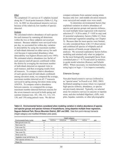Typically, we selected areas for extensive surveys in canyons or riparian areas, and also included ridgelines, cliffs, rock piles, bajadas, summits, or other physiographic Table 4.3. Environmental factors considered when modeling variation in relative abundance of species and species groups and species richness of herpetofauna, using stepwise multiple linear regression, Saguaro National Park, Rincon Mountain District, 2001 and 2002. Data from point-intercept transects (height category) and modified-Whittaker plots (plots). Height category Environmental factor (units) basal 0-0.5 m 0.5-2.0 m 2.0-4.0 m >4.0 m plot Bare ground cover (%) x Rock cover (%) x Forb cover (%) x x x Grass cover (%) x x x Tree cover (%) x x x x Shrub cover (%) x x x x Vegetation cover (all life forms, %) x x x x Plant species richness (no.) x Slope (%) x
features. We based extensive surveys on visual encounters (Crump and Scott 1994) and, in contrast to intensive surveys, did not constrain surveys by area or time. We focused extensive surveys during mornings and also surveyed during evenings and nights in low-elevation areas when detectability of snakes and amphibians is often highest (Ivanyi et al. 2000), and during midday at higher elevations. Field Methods We selected areas randomly and non-randomly (Table 4.1). We placed random survey areas within approximately 1 to 2 km of focal point transects, and surveyed each area once. We selected non-random areas by using topographic maps and prior knowledge of the district. We relied upon visual detection and often looked under objects and illuminated cracks to detect hidden individuals. We surveyed in spring (4 April – 24 May) and summer (25 June – 20 September) of 2001 and 2002. One, two, or three observers searched each area simultaneously and recorded data separately. Total duration of surveys among all observers combined averaged 5.5 ± 0.4 (± SE) hours per survey (range = 1.2 - 20.4 hours). We recorded data using similar methods as intensive surveys and noted UTM coordinates and elevation at the start and end points of each survey. Effort We surveyed 85 areas in 2001 and 2002 (Fig. 4.2), 94.1% of which were surveyed in 2001 (Table 4.2). Total survey effort was 465.2 hours, 81% of which was in non-random areas. Survey effort was roughly three times greater than for other methods and focused mainly during daylight except at lower elevations where we also surveyed during late evenings and nights. We did not survey higher elevation areas in late evenings and at night because detectability declined markedly with elevation. Analysis We calculated relative abundance for each area as the number of individuals detected for each species or all species combined per 10 hours of effort. For surveys completed by >1 observer 31 per area, we summed survey times and detection data for all surveyors when calculating effort and relative abundance for an area. Although some locations were surveyed multiple times, survey routes often varied and we therefore considered each survey an independent sample despite some spatial overlap. To describe general patterns of relative abundance for species groups (lizards, snakes, and amphibians) and species richness across the district, we post-stratified survey areas by elevation (low = 6,000 feet) using the median elevation of all animal observations for each survey. We then tested for variation among strata using one-, two-, or multi-way ANOVA. Because relative abundance and species richness varied between day and night and no areas were surveyed during night at middle and high elevations, we limited comparisons only to days. To describe patterns of relative abundance of individual species across elevation, we used multiple linear regression. We transformed relative abundance values when necessary using log(x) or log(x + 1) to improve normality. Because patterns of relative abundance often varied with relative humidity (or cloud cover), season, and time of day, we adjusted for these factors when they explained variation (P ≤ 0.10) in relative abundance. To describe cloud cover, relative humidity, and temperature for each area, we averaged measurements taken at the beginning and end of each survey. To adjust for temporal variation in relative abundance and richness across time of day, we considered three time periods: day, late evening or night, or surveys that spanned portions of both periods (day equaled reference level). We considered 20-min before local sunset time as the cut-point between day and late evening or night surveys. To adjust for seasonal variation in relative abundance and richness, we considered two seasons, spring and summer (spring equaled reference level). Because relative humidity and cloud cover were strongly correlated (r = 0.76, P < 0.0001) we only adjusted for the factor that explained the most variation in responses.
Page 1: Powell, Halvorson, Schmidt Vascular
Page 4 and 5: U.S. Department of the Interior DIR
Page 7 and 8: Table of Contents Report Dedication
Page 9 and 10: Table 5.8. Number of breeding behav
Page 11 and 12: Figure 6.5. Locations of non-random
Page 13 and 14: Report Dedication Eric Wells Albrec
Page 15 and 16: Acknowledgements Thanks to Saguaro
Page 17 and 18: Executive Summary This report summa
Page 19 and 20: Chapter 1: Introduction to the Inve
Page 21 and 22: them out. This information, in conj
Page 23 and 24: communities and is especially usefu
Page 25 and 26: Chapter 2: Park Overview Brian F. P
Page 27 and 28: Figure 2.2. Aerial photograph showi
Page 29 and 30: Figure 2.4. Diagram of the major ve
Page 31: Non-native Species and Changes to V
Page 34 and 35: General Botanizing Methods We colle
Page 36 and 37: Figure 3.3. Locations of modified-W
Page 38 and 39: Focal-points: General Patterns We f
Page 40 and 41: Percent 120 100 80 60 40 20 0 Plant
Page 42 and 43: well (Swantek et al. 1999). The mos
Page 45 and 46: Chapter 4: Amphibian and Reptile In
Page 47: Figure 4.2. Locations of intensive
Page 51 and 52: B). Reptilian species included two
Page 53 and 54: Table 4.6. Relative abundance (mean
Page 57 and 58: Cumulative number of species 50 40
Page 59 and 60: elevation range of the district all
Page 61: in recent years due to sedimentatio
Page 64 and 65: Spatial Sampling Designs We establi
Page 66 and 67: Figure 5.2. Location of section bre
Page 68 and 69: the relative abundance by repeat-vi
Page 70 and 71: Analysis We report relative abundan
Page 72 and 73: with some pine trees, mostly pinyon
Page 74 and 75: Riparian Sonoran Desertscrub Oak Pi
Page 76 and 77: Table 5.5. Mean relative abundance
Page 80 and 81: Nest Adults carrying objects Other
Page 82 and 83: Cumulative number of species Cumula
Page 84 and 85: can impact other native plant and v
Page 87 and 88: Chapter 6: Mammal Inventory Don E.
Page 89 and 90: Figure 6.3. Locations of random (fo
Page 91 and 92: calculated relative abundance by pl
Page 93 and 94: Figure 6.5. Locations of non-random
Page 95 and 96: (2) Receiver triggers camera to tak
Page 97 and 98: Excluding the results for the white
Page 99 and 100:
Table 6.5. Number of photographs of
Page 101 and 102:
Cumulative number of species Cumula
Page 103 and 104:
point out that the pond at Manning
Page 105 and 106:
There is some suggestion that popul
Page 107 and 108:
Chapter 7: Literature Cited Albrech
Page 109 and 110:
Davis, R., and C. Dunford. 1987. An
Page 111 and 112:
Kirkpatrick, C., C. J. Conway, and
Page 113 and 114:
Rice, J., B. W. Anderson, and R. D.
Page 115:
orderlands. Pp. 15-16. In effects o
Page 118 and 119:
100 Family Scientific name Common n
Page 120 and 121:
Page 122 and 123:
Page 124 and 125:
Page 126 and 127:
Page 128 and 129:
Page 130 and 131:
Page 132 and 133:
Page 134 and 135:
Page 136 and 137:
Page 138 and 139:
Page 140 and 141:
Page 142 and 143:
Page 144 and 145:
Page 146 and 147:
Page 148 and 149:
130 Order Voucher Specimen (S), Fam
Page 150 and 151:
132 UA survey type Survey or specie
Page 152 and 153:
Page 154 and 155:
Page 156 and 157:
138 Survey type Documentation type
Page 158 and 159:
Voucher Collection type Taxon Speci
Page 160 and 161:
Appendix F. List of existing vouche
Page 162 and 163:
Taxon Common name Collectiona Colle
Page 164 and 165:
Appendix G. Mean frequency of detec
Page 166 and 167:
Species Total transects observed Lo
Page 168 and 169:
Oak Savannah Pine-oak Woodland Coni
Page 170 and 171:
Appendix I. Details of small-mammal
Page 172 and 173:
Random or Camera Number of Number o
Page 174:
156
show all

Details - CALS Networking Lab - University of Arizona

Create successful ePaper yourself

Delete template?

Save as template?