Computing Extremal Quasiconformal Maps - Technion

O. Weber & A. Myles & D. Zorin / Computing Extremal Quasiconformal Maps
3. Background
In our exposition we primarily focus on maps from plane
to plane. Due to conformal invariance, all concepts can be
easily generalized to surfaces of genus zero by mapping the
surface conformally to the plane. However, as we briefly explain
in Section 6 all concepts and the algorithm can be extended
to surfaces of arbitrary genus.
We will use complex coordinates in the plane, z = x + iy.
For an arbitrary (not necessarily holomorphic) differentiable
function f (z), the complex derivatives are fz = 1 2 ( fx − i fy)
and f¯z = 1 2 ( fx + i fy). We assume that for all maps these
derivatives are defined almost everywhere, and are squareintegrable.
For each complex number z we define a ma-
Re(z) −Im(z)
trix A(z) =
and a vector v(w) =
Im(z) Re(z)
(Re(w),Im(w)) ⊤ , so that zw corresponds to A(z)v(w).
Dilatation and quasiconformal maps. The little dilatation
of a differentiable map f at z is defined as
k(z) =
f¯z
fz
(1)
It is related to the ratio K of singular values of the Jacobian
of f (large dilatation) by K = 1+k
1−k . A map f : D → D′ is
quasiconformal if k(z) ≤ k for some k almost everywhere in
D. In this case, k( f ) = supk(z) is the maximal dilatation of
the map. The dilatation k has the following important properties:
• 0 ≤ k < 1 for orientation-preserving maps, and 1 ≤ k ≤ ∞
for orientation reversing maps.
• for a conformal map k = 0 and a conformal map composed
with reflection k = ∞.
An advantage of considering k instead of K is that k varies
continuously as the sign of the determinant of the Jacobian
of f changes on folds, while K has a singularity (cf. comparison
of functionals in Section (2)).
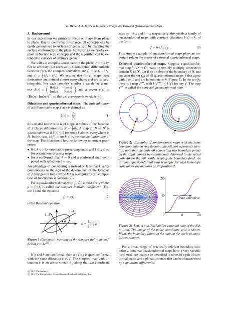
For a quasiconformal map with fz = 0 almost everywhere,
µ = f¯z/ fz is called the complex Beltrami coefficient, (Figure
1) and the equation
is the Beltrami equation.
1–k
f¯z = µ fz
θ
1+k
θ = 1
arg μ
2
Figure 1: Geometric meaning of the complex Beltrami coefficient
µ = ke 2iθ .
If g and h are conformal, then h ◦ f ◦ g is quasiconformal
with the same dilatation k as f . The simplest map with dilatation
k is an affine stretch Ak along the two coordinate
c○ 2012 The Author(s)
c○ 2012 The Eurographics Association and Blackwell Publishing Ltd.
(2)
axes by 1 + k and 1 − k respectively; this yields a family of
quasiconformal maps with constant dilatation k(z) = k, of
the form
f = h ◦ Ak ◦ g. (3)
This simple example of quasiconformal maps plays an important
role in the theory of extremal quasiconformal maps.
Extremal quasiconformal maps. Suppose a quasiconformal
map h : D → D ′ maps a (possibly multiply connected)
domain D to D ′ . Let B be a subset of the boundary of D, and
consider the set QB of all quasiconformal maps f that agree
with h on B and are homotopic to h (Figure 2). In the set QB
there is a map f ext , with k( f ext ) ≤ k( f ) for any f . The map
f ext is called the extremal quasiconformal map.
A
B
Figure 2: Examples of nonhomotopic maps with the same
boundary data on ring domain; the left plot represents identity;
note that the path AB connecting two boundary points
on the right, cannot be continuously deformed to the spiral
path AB on the left, while keeping the boundary fixed. An
extremal quasiconformal map is unique for each homotopy
class under assumptions of Proposition 2.
2π
π
0
A
B
zero derivative
Figure 3: Left: A non-Teichmüller extremal map of the disk
to itself. The image of the polar coordinate grid is shown.
Right: the boundary values of the map on the circle in angular
coordinates.
For a broad range of practically relevant boundary conditions,
extremal quasiconformal maps have a very specific
local structure that can be described in terms of a pair of conformal
maps, and a global structure that can be characterized
by a quadratic differential.
π
2π